Bayesian progress curve analysis of MicroScale thermophoresis data

Abstract

MicroScale Thermophoresis (MST) follows the movement of fluorescent-labelled biomolecules with different sizes along a temperature gradient. The presence of a “contrary trend” pattern, that is, the trend of fluorescence change reversing at higher titrant concentrations, is a well-known problem with uncertain cause. Conventionally, binding curves and kinetic parameters are derived from MST datasets using regression analysis on isolated time windows, while the rest of the data are ignored, and the “contrary trend” fluorescent levels are also usually removed as outliers. This biased approach can be avoided with a more continuous analysis of the entire kinetic process. The Bayesian model of MST progress curves allows the inference of parameters and modelling of the whole experiment. The removal of unusual data points is unnecessary once the anomalous kinetic process is identified. This alternative data analysis approach was applied to our MST datasets from survivin–hSgol2 interactions, and the results show that the binding curves remained sigmoid when all data were included. We were also able to infer the value and uncertainty of the dissociation constant (K_D) by ascribing the anomalous data points to a new, linear kinetic component. This approach demonstrates good posterior predictions from the MST process in both short and longer experiments as well as the feasibility of K_D inference from short experiments.

---

Introduction

MicroScale Thermophoresis (MST) allows the quantification of molecular interactions based on their movements along a microscopic temperature gradient and other temperature-dependent physical processes affected by ligand binding. It permits the detection of subtle changes in molecular properties that are affected by a binding event.¹ The empirical analysis of MST data is especially valuable to observe biomolecular interactions, such as those between proteins, wherein a sensitive method is needed to see small changes on the molecular surface or at the molecule–solvent interface.²

An MST experiment is commonly performed by mixing a fluorescent-labelled molecule (target) with an unlabelled molecule (ligand) at multiple concentrations (typically from nanomolar to millimolar concentrations). The mixture is then incubated for some time before it is placed in a capillary tube. Fluorescent labelling is necessary for monitoring the amount of target in the laser focus and observing the time-dependent changes in fluorescence intensity. It is possible to use the intrinsic UV fluorescence of aromatic amino acid residues in the target using a specialized instrument, but that excludes ligands that also produce UV fluorescence (for example, when the ligand is also a protein). Different ligand concentrations would give rise to a wide range of fluorescence intensities and mask the fluorescence of the target.

To create a temperature gradient, an infrared laser is directed towards a region in the capillary tube. As the molecules respond to the temperature change and diffuse away from the spot, the change in fluorescence signal in the illuminated region is recorded over time, resulting in fluorescence time traces. These are normalized to the initial fluorescence intensity (F_normal). For the determination of the dissociation constant (K_D), the target concentration is kept constant and low, while the ligand concentration is varied and acts as the titrant. The dissociation constant is considered to be:

where [L], [T] and [LT] are the concentrations of the ligand, unbound target and ligand–target complex (the bound form of the target), respectively.

This results in a mixture of unbound and bound forms of the target. Selected regions of the raw fluorescence time traces are further analysed, and in an ideal case, the average intensities in these regions result in sigmoidal binding curves, with F_normal as a function of the ligand concentration.^1,3

Currently, few tools are available to analyse the time traces and convert them into a binding curve, including MO.Affinity Analysis from NanoTemper Technologies and the open-source software PALMIST developed by Scheuermann et al.³ Both tools divide the distinctly shaped time trace pattern into separate regions: a steady-state period before the temperature gradient is applied, a short period after the temperature gradient is applied (the “temperature-jump”), and a later thermophoresis steady-state period.³ MO.Affinity Analysis calculates the F_normal of the binding curve by normalizing fluorescence at the later steady-state to that at the initial steady-state before illumination. The tool also enables advanced users to modify the region range in a time trace dataset. Scheuermann et al. found that calculating F_normal from (F_h − F_c)/F_c, introduced more noise to their data (where F_h is the fluorescence at the later steady-state or “hot” region, and F_c is the fluorescence at the “cold” early time). They used another approach by calculating F_normal from F_h/F_c to get a better signal-to-noise ratio in PALMIST.^3,4F_normal is an important parameter because it is the primary data used for modelling the binding curves in the traditional data analysis framework. Although the cold relative fluorescence level is supposed to be close to 1, random and systematic errors affect it. It is important to note that time plays a limited role in traditional analysis; only the fluorescence levels before and after a certain time interval are compared.

Scheuermann et al. later improved the confidence interval for K_D estimation with error surface projection (ESP) by comparing it with other methods, such as the analysis of the variance–covariance matrix, Monte Carlo simulation, and bootstrapping. ESP thoroughly checks the error surface considering that defects in a specific parameter may be covered up by other parameters. Users may also choose a suitable combination of the time trace regions for fitting the binding curve according to the expected binding mode of the interacting molecules. The “temperature-jump” region, for example, may not be used to detect molecular interactions that do not directly affect the fluorescent dye.³ Tso et al. added two new models to calculate the F_normal of molecules with a 1 : 2 binding mode better, which have been implemented in the most recent version of PALMIST. One model involves splitting the binding curve into two and analysing them separately; this requires more sampling points to cover an adequate range of concentrations in each sub curve. Another model assumes a symmetrical bivalent molecule to account for the cooperative binding sites. Both approaches require the user to have prior knowledge of the expected binding mode.⁵

While improvements to the analytic tools were made, Scheuermann et al. also documented a peculiar “contrary trend” pattern. In MST experiments carried out to describe the DVD-Actin/VCA′* interaction, the F_normal value increased as more titrant was added to the sample mix. However, higher titrant concentrations showed a reversal in trend, with the F_normal decreasing instead. This reversal was also observed in a simulated 1 : 2 binding interaction when the dataset was fitted to a model assuming a symmetrical bivalent binding partner. Tso et al. noted that trend reversal or a second inflection point at high titrant concentrations might not necessarily come from binding.⁵ In the case of DVD-Actin/VCA′*, the cause of such a reversal in the pattern is unknown. At the moment, users of both PALMIST and MO.Affinity Analysis may opt to remove the data points manually so as not to skew the fitted curve, which happens when the observations clearly do not follow a random normal distribution.³ Besides introducing a bias, this approach also does not explain why such ‘outliers’ exist, to begin with. An alternative approach is using robust distributions in a Bayesian framework to analyse the MST binding curves, as described previously for survivin and human Shugoshin-like protein (hSgol) interactions.⁶ For several error models, robust Bayesian curve fitting is visually better and needs lesser repetition to reach a similar level of precision as the standard regression approach. The robust curve fitting of survivin–hSgol interactions shows that the model captures the central tendency of the data even without removing the contrary data points.⁶

Progress curve analysis is mostly associated with recording the progress of the chemical reaction dynamics and solving equations to describe continuous reaction kinetics. It has the advantages of inferring parameters using the whole kinetic curve and requiring fewer repeats to estimate these parameters. The limited usage of progress curve analysis is often attributed to its complex mathematical modelling. Increasing advancements in computational power, however, have enabled the integration of rate equations and optimization of their parameters to fit the experiment progress curves.^7,8 The optimization of parameters and estimation of the uncertainty of parameters can be performed in a Bayesian framework, which is uncommonly used for inference in progress curve analysis. The Bayesian inference has recently been adapted to describe complex biophysical systems; it uses a continuously self-refining model as more data are added to improve the accuracy and precision of the model.⁹ By learning from a wide variety of training datasets, the model progressively makes better estimations on the actual dataset. The continuous learning nature of Bayesian inference makes it highly suitable for pairing with the diverse experimental conditions in progress curve analysis. Choi et al. showed that, after applying Bayesian inference on enzyme reaction dynamics with diverse kinetics, the bias in the progress curves was significantly reduced compared with conventional regression. The conventional model showed a rise in errors in the posterior samples with increased enzyme concentrations. Meanwhile, the posterior samples from the progress curve model were consistently more accurate.¹⁰ The ideal process of thermophoresis is not equivalent to the changes in concentration in a chemical reaction for which progress curve analysis is applied previously. The empirical progress of diffusion and other (photochemical) processes can be modelled with independent exponential (and linear) components even during a thermophoresis experiment. Therefore, we keep using the term progress curve analysis in a general sense and not limited only to modelling chemical reaction kinetics.

Here, we show that a certain type of anomalous MST data can be successfully modelled with the addition of a single linear kinetic parameter together with the exponential process that is typically attributed to thermophoresis and binding-dependent fluorescence change. Through progress curve analysis, we have identified a new kinetic component that corresponds to the contrary trend observed previously. By applying Bayesian progress curve analysis to our MST data, we were able to extract the kinetic parameters without having to remove any outliers, as well as determine more precise K_D values than those determined by traditional regression analysis. We could also quantify the uncertainty of K_D obtained from the hierarchical Bayesian framework. Our results show that the fitting of MST traces from short experiments had a similar quality to those from longer ones and presented reproducible posterior sample predictions. Although the K_D posterior probability distribution of the short experiments was understandably broader, the location of the posterior peak was identical to that obtained in longer experiments. In practice, this would allow us to use shorter MST time traces to estimate K_D.

Results and discussion

Raw normalized fluorescence (F_normal) time traces potentially contain more information even if the shape of the progress curve radically deviates from the expected shape. The initial levels of fluorescence are expected to be invariant, but photobleaching, chemical and/or physical processes affecting fluorophores can influence the F_normal change even before the IR laser irradiation is initiated. It is not unreasonable to believe that the initial trend may continue to the heating phase of the experiment. After heating the laser spot, F_normal progress curves must ideally display a biphasic exponential decay. The final fluorescence level does not always reach a new steady-state during the experiment due to several factors (limited experimental time, photobleaching, and potential thermal denaturation of reaction components). The actual final fluorescence keeps changing as the longer the experiment is recorded, and the final fluorescence does not reflect the exponential amplitude.

Fast decay is usually associated with a temperature effect on the yield of the fluorophore itself, which may or may not be affected by the altered chemical environment upon complex formation. In the shown example (Fig. 1a), the fluorescent labels are chemically attached to survivin, and the peptide could make direct contact with the fluorophore. The slow decay is assumed to represent the thermophoretic movement, which is a diffusive process. It is modified by the size, charge, and shape changes occurring in the protein and/or in the hydration shell upon complex formation.

Fig. 1 Experimental MST data. (a) Primary thermophoresis data from serial dilutions of hSgol2 peptide when incubated for 5 min with fluorescent chemical-labelled survivin. The cold (−3 to −1 s) and hot (27–29 s) regions used to analyse the thermophoresis binding curves are represented by blue and red vertical lines, respectively. (b) Thermophoresis binding of hSgol2 at varied hSgol2 concentrations. The blue dots represent measurements obtained from a dilution series.⁶

There are many potential advantages of the (Bayesian) thermophoretic progress curve analysis. For example, one can estimate the exponential amplitudes from a continuous curve without limiting the analysis to the comparison of arbitrarily selected regions in the curve (Fig. 1). The early time points are more valuable and carry information about both exponential processes. Thus, one may even consider ending the experiment before a steady-state fluorescence level is reached. A trivial advantage is that one can perform the experiment faster, but it may also be practically impossible to reach a steady-state fluorescence level. Besides those caused by photobleaching, there are other yet unexplained drifts (modelled with linear time dependence in the absence of a better kinetic model) that continue to act on longer timescales after the exponential T-jump and even when the thermophoretic processes are practically over. We show evidence for this by modelling the progress curves in Fig. 2a.

Fig. 2 Bayesian MST progress curve analysis. (a, b) Primary thermophoresis data (grey) on hSgol2 interaction after (a) 30 s and (b) 9 s of heat induction. These traces represent the unbound peptide at 15.3 nM (blue), bound peptide at 500 μM (green), and an example of an anomalous experiment at 1.5 μM (orange). The dark lines are the medians of the predicted F_normal distributions, and the lightly shaded areas are the highest density interval (HDI 95%) of the predicted F_normal distributions. (c) A posteriori distribution of K_D inferred from the 30 s (green) and 9 s (blue) thermophoresis data.

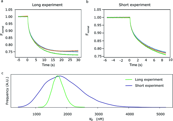
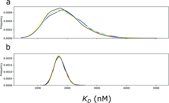
In Fig. 2, we have compared the fit of a short experiment curve (9 s; Fig. 2b) with a fully recorded (30 s; Fig. 2a) progress curve and the inferred K_D distributions. As expected, the probability distribution of the exponential amplitudes and K_D parameters inferred from the 9 s curves were broader compared with the 30 s curves, but for most practical purposes, 9 s is sufficient. The mean of K_D posterior distribution determined for the long experiment was 1.8 μM (s.d. 0.18 μM), which is in line with a robust analysis method described previously on a triplicate of observations (1.6 μM).⁶

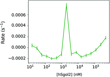
In Fig. 3, we have compared the influence of ligand concentration on the magnitude of the linear kinetic constant in a fully recorded experiment. At 2 μM hSgol2 peptide concentration, an anomalously large positive gradient value was seen, which forces the progress curve to keep increasing without reaching a steady-state level. At 30 s, the F_normal value was higher than the presumably fully unbound survivin when 15 nM hSgol2 peptide concentration was applied.

Fig. 3 Rate constants based on the linear kinetic component for each concentration of hSgol2 peptide when mixed with fluorescent chemical-labelled survivin in a 30 s heating experiment. The rate constants of hSgol2 interaction do not seem to have a sigmoid function with the ligand concentration. At 2 μM concentration of the hSgol2 peptide, an anomalous rate constant can be observed. The vertical bars represent the highest density intervals (95%) of the a posteriori rate constants.

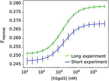
Disregarding this linear background process described by one parameter per curve, the total exponential amplitudes were perfectly sigmoid, as required by the theory (Fig. 4), while the posterior predictions remained remarkably good for all progress curves in the experiment (Fig. 2a). The nominal value of F_normal may look very unusual towards the end of the experiment, but the total amplitude of the exponential components, and their rates were in line with the equivalent parameters at adjacent ligand concentrations. The linear components showed a concentration-dependent tendency: the gradient increased above 0 both towards the high and low ends of the ligand concentration range. The observation of a near-linear component is not rare. Scheuermann et al. showed a “contrary trend” when studying the DVD-Actin/VCA′* interaction.³ In their study, F_normal returned to an intermediate level in a strong near-linear manner at high VCA concentrations. A common practice is to remove these contrary data points at high ligand concentrations from the binding curves. Unfortunately, this procedure does not solve the problem, because the “contrary trend” is already present at other concentrations. We could see this smooth variation directly in our data and, if left untreated, this linear trend influences the obtained K_D values. A routine solution is to make the analysis of binding curves robust against seemingly anomalous occurrences.⁶ Alternatively, by thermophoretic progress curve analysis, one can attempt to isolate the interesting kinetic components of thermophoresis from the kinetic background. The process of learning is not only to recognize but also to be able to focus on the relevant core details. The hierarchical nature of this Bayesian network makes it especially sensitive to exponential processes and sigmoid concentration dependence of ligand binding. Every other process that does not fit this framework is not considered relevant. Progress curve analysis is powerful but requires more computational resources, and the MST progress curves sometimes defy even very general expectations. Fortunately, in the described case, a linear time-dependent kinetic background could be used, which already extends the potential range of the curve.

Fig. 4 Total exponential amplitudes of the fitted model for the MST data from the hSgol2 interaction experiments. It represents the total amplitude of the fast and slow exponential components together from the 9 s (blue) and 30 s (green) experiments, after the application of the linear background process. The presence of anomalous linear rate constants does not affect the total exponential amplitude. The vertical bars represent the highest density intervals (95%) of the a posteriori total amplitudes.

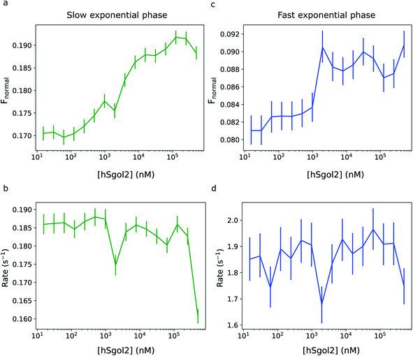
Fig. 5 shows the comparison of the exponential phase amplitudes inferred from the MST data involving the interaction of chemically labelled survivin and the hSgol2 peptide. Both amplitudes showed a correlation with the ligand concentration, and for the fast phase, the transition appeared at a lower ligand concentration. The magnitude of rate constants did not seem to correlate with the ligand concentration in both the fast and slow exponential phases.

Fig. 5 Comparison of the fast and slow exponential phases of the MST data for hSgol2 interaction in the 30 s heating experiment. (Top) Comparison of the (a) slow and (c) fast exponential component amplitudes of the hSgol2 interaction. The amplitude of the slow exponential phase is almost two times higher than that of the fast exponential phase. (Bottom) The exponential rate constants of the (b) slow and (d) fast exponential components of hSgol2 interaction are almost constant at all ligand concentrations. The rate constants do not seem to correlate with hSgol2 concentration as the amplitudes do. However, anomalous rate constants can be observed at hSgol2 peptide concentrations 2 μM and 500 μM in the slow exponential phase. The vertical bars represent the highest density intervals (95%) of the (a, c) a posteriori exponential amplitudes and (b, d) rate constants, respectively.

Clearly, there is room for further improvement of the thermophoretic progress curve analysis. We were only partly correct with our assumption that the linear background process is common in the pre- and post-heating phases of the experiment. In most cases, the preheating trace is not necessary for the accurate estimation of the post-heating trend; however, it may be worth linking them together with a common hyper-parameter.

Experimental methods

Sample preparation and labelling

Survivin was expressed and purified as described by Garcia-Bonete et al.⁶ The hSgol2 peptide (ECQVKKVNKMTSKSKKRKTS) was chemically synthesized (Genscript). Survivin was chemically labelled with the MO-L005 Monolith™ Protein Labelling Kit GREEN-MALEIMIDE (Cysteine Reactive) from NanoTemper Technologies, and the MST experiments were performed in a buffer with 50 mM Tris pH 8.0, 150 mM NaCl, 1 mM DTT and 0.05% Tween. The hSgol2 peptide was diluted and titrated in the same buffer.

MicroScale thermophoresis

The MST experimental data have been published previously;⁶ here, we only provide a short summary of the relevant details. The MicroScale thermophoresis experiments were performed according to the protocol prescribed by NanoTemper Technologies in a Monolith NT.115 (green/blue) instrument (NanoTemper Technologies) using the green channel. Serial dilutions of the hSgol2 peptide (ECQVKKVNKMTSKSKKRKTS) were obtained using the buffer containing 50 mM Tris pH 8, 150 mM NaCl, 1 mM DTT buffer with 0.05% Tween. The experiments were carried out at 24 °C.

After serial dilution and incubation for 5 min, the experiments were performed using 20% MST power and 40% LED power. The MST traces were recorded using the standard parameters: 5 s MST power off, 30 s MST power on (these two periods were used for the progress curve analysis) and 5 s MST power off.

Probabilistic modelling of MST progress curves

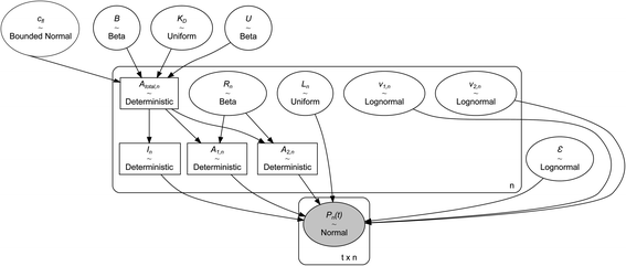
The experiments modelled here included a 5 s preheating fluorescence recording and a 30 s total post-heating time trace. As a test, the post-heating period of the same data was also truncated to 9 s. Our extended kinetic model consisted of global and local random variables. Fig. 6 illustrates the connectivity of the Bayesian network.

Fig. 6 Simplified illustration of the Bayesian network. The names of the variables are the same as mentioned in the Methods section. The experimental data consist of time traces recorded on n = 16 capillaries containing t = 475 time points (30 s). The variables enclosed in ellipses are stochastic, while the rectangular variables are deterministic i.e., their distributions completely depend on the distribution of the connected variables. The arrows indicate the dependency of variables on each other. The posterior distribution of the variables is determined by the frequency at which their joint values appear during MCMC sampling. This frequency corresponds to the product of likelihood and the independent prior distributions according to the Bayes formula once the MCMC sampling reaches a steady state. As with all Bayesian inference problems, the data values are assigned to a distribution and kept fixed and indicated by the shaded ellipse. This figure is generated using the python library Graphviz and modified using the Inkscape software.

K _D is a global variable with the same a priori expectations as described previously (eqn (2)).⁶ Likewise, the probability distribution of fluorophore concentration is identical (eqn (3)). U and B represent the pure total amplitudes of the exponential processes for the unbound and fully bound fluorophores, respectively. It is also possible to change the definition of U and B to link them to the amplitude of only one of the exponential components.

The a priori assumptions for U and B were identical and described by a flat β distribution. By assuming positive amplitudes, we ensured that fluorescence would not increase beyond the initial level due to exponential (T-jump and thermophoretic) processes (we leave that possibility open through a linear process though). Not fully bound fluorophores at ligand concentrations c_n have intermediate exponential amplitudes A_total,n determined by the law of mass action, and are entirely the deterministic combination of the stochastic components above:

The experimental data were modelled as part of a normal distribution, and its scale parameter ε was a single global variable with a lognormal a priori distribution in our model. This choice was motivated by the belief that the errors do not vary from capillary to capillary.

Local random variables were linked to each of the n thermophoretic progress curves, and their models consisted of one linear and two exponential components. The linear process was modelled from the beginning of the fluorescent signal recording, and the exponential processes started from IR laser irradiation:

L_n(t) = ν_0,n(t + 5 s) (8)

E_1,n(t) = A_1,ne^−ν_1,nt (9)

E_2,n(t) = A_2,ne^−ν_2,nt (10)

Since A_total,n = A_1,n + A_2,n, they can be linked together with a single, curve-associated random ratio parameter (R_n) varying between 0 and 1. R_n can be conveniently modelled with a β distribution, and a slightly asymmetric prior expectation would ensure that exponential processes with larger and smaller amplitudes are grouped together for comparison.

E_1,n(t) = R_nA_total,ne^−ν_1,nt (11)

E_2,n(t) = (1 − R_n)A_total,ne^−ν_2,nt (12)

Since the progress curves were normalized to 1 at t = −5.0 s, the final fluorescence level approached by the two exponential components in an ideal experiment (i.e., an experiment without the linear component) was I_n = 1 − L_n(5.0 s) − A_total,n.

The remaining rate parameters were modelled as random variables with the following a priori parameters for the uniform and lognormal likelihood functions:

Before t = 0 s, the progress curves were modelled as:

where μ and ε correspond to the location and scale parameter of the normal distribution (one global scale parameter).

When t ≥ 0 s, the progress curves were modelled as:

Before sampling the posterior parameter space, the model was scaled by the Automatic Differentiation Variational Inference (ADVI)¹¹ algorithm, and subsequently, 7000 samples were collected in four parallel chains using the No-U-Turn Sampling algorithm (NUTS).¹² Notably, ADVI was not the default scaling method, and the default jitter+adapt_diag method failed to provide a suitable starting point. The model parameters in the last 5000 samples exhibited steady-state fluctuations around the a posteriori maximum and converged to identical distributions in the four parallel sampling processes (Fig. 7). For the final analysis, the 5000 samples from the four chains were merged to yield 20 000 samples.

Fig. 7 Four MCMC chains of the KD parameter is shown for modelling (a) the short and (b) the long experiments. The kernel density estimates of the four chains are indicated with yellow, magenta, cyan and blue colors. The independant sampling of the chains converged to very similar distributions.

The computational speed was around 1.9 iterations per s on a Linux workstation (i7-3970X CPU at 3.50 GHz clock frequency), with four parallel chains growing at each iteration. An interactive implementation is available through Google's Colab, on the link: https://colab.research.google.com/github/Katona-lab/MST-analysis/blob/main/MST_progress_curve_analysis.ipynb.

At a typical load in a CPU-only Colab environment, the MCMC sampling performance was approximately 1.6 iterations per s, and it was growing only one chain at a time. The posterior samples were also used for 1000 new predictions. These posterior predictive samples were demonstrated by their median and their highest density interval (95%) at each time point on the progress curve.

Conclusions

We have demonstrated that Bayesian progress curve analysis gives more insights from anomalous data points in MST time traces, which are typically considered outliers in conventional regression analysis. Once the linear component is identified and accommodated, the total exponential amplitude can be fitted assuming perfect sigmoid curves. Hierarchical models are very difficult to implement using non-linear regression methods, and it is practically impossible to estimate the robustness of the model parameters. While our Bayesian framework shows a broader posterior distribution of K_D at shorter observation times, the peak location is useful for K_D estimation.

Data availability

Data used for processing scripts in this paper is available, see https://doi.org/10.5281/zenodo.6379340.

Author contributions

MJGB and GK designed experiments, ALA, GK, and MB wrote the main manuscript text, MJGB prepared the figures. MJGB and MJ performed experiments, ALA, MJGB, CVR, and GK analysed data. All authors reviewed the manuscript.

Conflicts of interest

There are no conflicts to declare.

Acknowledgements

The authors wish to thank the Åke Wiberg Foundation and the Röntgen-Ångström Framework (award no. 2015-06099) for their support. This work was also supported by the Swedish Research Council (award no. 2017-03025), and the Inga-Britt and Arne Lundberg Foundation.

Notes and references

1. M. Jerabek-Willemsen, et al., Molecular interaction studies using microscale thermophoresis, Assay Drug Dev. Technol., 2011, 9(4), 342–353.
2. C. J. Wienken, et al., Protein-binding assays in biological liquids using microscale thermophoresis, Nat. Commun., 2010, 1, 100.
3. T. H. Scheuermann, et al., On the acquisition and analysis of microscale thermophoresis data, Anal. Biochem., 2016, 496, 79–93.
4. S. Lippok, et al., Direct detection of antibody concentration and affinity in human serum using microscale thermophoresis, Anal. Chem., 2012, 84(8), 3523–3530.
5. S. C. Tso, et al., Using two-site binding models to analyze microscale thermophoresis data, Anal. Biochem., 2018, 540–541, 64–75.
6. M.-J. Garcia-Bonete, et al., Bayesian Analysis of MicroScale Thermophoresis Data to Quantify Affinity of Protein:Protein Interactions with Human Survivin, Sci. Rep., 2017, 7, 16816.
7. R. G. Duggleby, Progress-curve analysis in enzyme kinetics. Numerical solution of integrated rate equations, Biochem. J., 1986, 235(2), 613–615.
8. N. Nikolova, K. Tenekedjiev and K. Kolev, Uses and misuses of progress curve analysis in enzyme kinetics, Cent. Eur. J. Biol., 2008, 3(4), 345–350.
9. K. E. Hines, T. R. Middendorf and R. W. Aldrich, Determination of parameter identifiability in nonlinear biophysical models: A Bayesian approach, J. Gen. Physiol., 2014, 143(3), 401–416.
10. B. Choi, G. A. Rempala and J. K. Kim, Beyond the Michaelis–Menten equation: Accurate and efficient estimation of enzyme kinetic parameters, Sci. Rep., 2017, 7(1), 17018.
11. A. Kucukelbir, et al., Automatic variational inference in Stan, in Advances in neural information processing systems, 2015.
12. M. D. Hoffman and A. Gelman, The No-U-Turn Sampler: Adaptively Setting Path Lengths in Hamiltonian Monte Carlo, Journal of Machine Learning Research, 2014, 15, 1593–1623.

---

Footnote

† These authors contributed equally to this work.

---