 Open Access Article
Graph neural networks for the prediction of infinite dilution activity coefficients†
Edgar Ivan
Sanchez Medina
 a,
Steffen
Linke
 a,
Martin
Stoll
b and
Kai
Sundmacher
 *ac
*ac
aChair for Process Systems Engineering, Otto-von-Guericke University, Universitätsplatz 2, Magdeburg, 39106, Germany
bChair of Scientific Computing, Department of Mathematics, Technische Universität Chemnitz, 09107 Chemnitz, Germany
cProcess Systems Engineering, Max Planck Institute for Dynamics of Complex Technical Systems, Sandtorstraße 1, Magdeburg, 39106, Germany. E-mail: sundmacher@mpi-magdeburg.mpg.de
First published on 11th February 2022
Abstract
The use of predictive methods for physicochemical properties is of special interest given the difficulties involved in the experimental determination of large chemical spaces. In this work, we focus on the prediction of infinite dilution activity coefficients γij∞ of organic systems using graph neural networks (GNNs). Our proposed method involves the use of one GNN that extracts the relevant solvent information and one GNN for doing so for the solute. The vectorial representations of these chemical species are then combined into a binary-system fingerprint which is used as the input to a supervised learning framework. We compare our approach to the 8 most commonly employed phenomenological/mechanistic methods for predicting γij∞. Our method is able to predict γij∞ with competitive performance to the state-of-the-art mechanistic methods, achieving a lower mean absolute error (MAE) compared to the broadly used COSMO-RS and UNIFAC-Dortmund methods. We also present a series of parallel residual hybrid models that combine both mechanistic and GNN-based approaches. These hybrid models overall improve the performance of the individual model instances.
1 Introduction
Mathematical models are largely used in chemical process design and optimization. These models often require that physicochemical data of the involved chemical species is available. Collecting such data is expensive and time-consuming, and, as a matter of fact, it is an impossible task to accomplish for the enormous chemical space of interest.1 This problem has historically motivated the development and application of predictive methods.One thermodynamic property of special interest is the so-called activity coefficient γ, which measures the degree of nonideality of a substance in a liquid mixture due to intermolecular or intramolecular forces. Naturally, γ depends on the temperature and composition of the mixture (i.e., pressure dependence can be neglected in most cases), and for each temperature the limiting case occurs when a solute i is infinitely diluted in a solvent j. The activity coefficient at these conditions is denoted as γij∞. Its importance for chemical processes is very broad because separation processes achieving high product purities reach approximately infinite dilution conditions. Furthermore, in distillation, γij∞ is used to predict whether an azeotrope is expected to occur or not.1,2 And in liquid–liquid extraction, the selection of a suitable solvent is often based on γij∞ values.3,4 Moreover, γij∞ plays a major role for safety and environmental protection studies.4,5
Many models exist that are used for the prediction of γij∞. We can divide these models into the ones based on mechanistic or phenomenological knowledge6–13 (refer to as mechanistic models in this work), and those which are mainly constructed using machine learning techniques.14–21 So far, the use of mechanistic models is more common compared to machine learning methods. The reason for this is that mechanistic models have been developed, studied and tested for decades as opposed to the machine learning approaches. However, many deviations from reality are still present in mechanistic models.22 For instance, in the system methylcyclohexane–toluene as solute and acetophenone as solvent deviations larger than 41% are still encountered23 when using UNIFAC-Dortmund (the recommended mechanistic model for such type of compounds according to the literature22). The reader is referred to the work of Brouwer et al.22 for a detailed explanation of the current limitations of mechanistic models. With the recent advances in computational power and the digitization of large databases, data-driven methods are becoming an interesting focus of research in this context.18,21,24–26
The most commonly used mechanistic models for predicting activity coefficients can be grouped into 4 categories: solvation models,6–8,27,28 group contribution methods,9–11,29–32 linear solvation relationships12,33–37 and COSMO-RS.13,38,39 A recent work22 re-visited the main eight models in these categories and compared them in the context of predicting γij∞ at 298.15 K. Solvation models are based on the Flory–Huggins theory27,28 and include the (1) Hildebrand model,6 (2) Hansen Solubility Parameters (HSP),7 and the (3) Modified Separation of Cohesive Energy Density (MOSCED) model.8 Similarly, most common group contribution methods are also constructed on modifications of the Flory–Huggins model, and are mostly represented by (4) UNIFAC9 and the modification thereof, known as (5) UNIFAC-Lyngby10,29 and (6) UNIFAC-Dortmund.11,30–32 Linear solvation energy relationships combine solute and solvent descriptors using multilinear regression. The most prominent instance of such models is the one developed by (7) Abraham.12 By contrast, (8) COSMO-RS13,38,39 is based on quantum mechanical calculations and molecular energy interaction estimations (i.e., the resulting surface charges of the individual molecules are energy-optimal paired to an interaction model).
Many of the machine learning methods that have been developed for predicting infinite dilution activity coefficients have been built as quantitative structure–property relation (QSPR) models.14–19 For constructing such models typically two steps are necessary: (1) molecular descriptors selection and (2) training of a regression method (e.g., linear regression, support vector machines, artificial neural networks). In this approach many quantum-chemical and/or topological descriptors are calculated and discarded for not being relevant enough for an accurate prediction. A notable exception to this was the application of the matrix completion methodology (MCM) that allows for the predictions to be based only on an incomplete matrix of solvent–solute activity coefficients.21,40,41 This eliminates the necessity of computing many expensive descriptors. However, the application domain of the MCM method is limited to the systems that define the matrix. Also, the accuracy of the predictions heavily depends on the correlation and the amount of the available data.41 A common limitation of both QSPR and MCM methods available in the literature is that no information on the uncertainty of the predictions is provided (i.e., no error bars are usually reported).
In similar contexts of molecular property prediction, graph neural networks (GNNs) have shown promising results, achieving state of the art performance on several applications.42–45 In this framework, a molecule is represented as a graph with nodes and edges defined by the atoms and chemical bonds, respectively. Additionally, in the context of predicting γij∞ one molecule acts as the solute while the other acts as the solvent. The structural differences and the molecular interactions between the solute and solvent naturally affect the value of γij∞. The principal contribution of this paper is precisely to investigate the use of GNN-based models for predicting γij∞ of organic solvent/solute systems at a constant temperature, and to compare the GNN predictions to the 8 most relevant mechanistic approaches described above. By using GNNs the system descriptors are automatically learned in an end-to-end fashion using backpropagation and predictions can be obtained to systems that are not included in the training set. We also explore the use of ensemble learning and hybrid modeling in order to develop residual GNNs that can potentially be used for explainability. To the best of our knowledge, GNNs have never been used for this purpose.
2 Methods
2.1 Data sources
The data used in the present study is available in the literature (see ESI† for a complete reference list) and was collected in the work of Brouwer et al.22 This database consists of experimentally determined infinite dilution activity coefficients at 298.15 K. The data was collected using non-analytical techniques (e.g., comparative ebulliometry, comparative tensimetry and dew-point temperature determination) in some cases, whereas in others analytical methods (e.g., retention measurements in GLC, headspace analysis method, static mass balance methods, rate measurements on continuous gas–liquid separation processes and distillation methods) were employed. Clearly, analytical methods provide better confidence ranges compared to non-analytical studies. However, given the scarcity of the available data and the consistent lack of reported confidence intervals in the literature, both collection techniques were considered in this work.2.2 Data cleaning
The original database22 consists of 4460 data points from binary substances pairs of 156 solutes and 262 solvents. However, among these points there are multiple entries referring to the same system. The number of covered different systems therefore reduces to 2810 (i.e., 6.9% of the complete considered binary space, see Fig. 1). Therefore, a cleaning step was performed by taking the arithmetic mean of the repeated entries. A clear description of these cases can be found in the ESI.† For scaling purposes the ln(γij∞) was used instead of the γij∞-values. These scaled activity coefficients appear naturally when calculating the chemical potentials.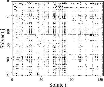 | ||
| Fig. 1 Schematic representation of all possible binary mixtures formed by the 156 solutes and 262 solvents considered in this work. The black squares indicate mixtures for which experimental data on γij∞ at 298.15 K is available within the studied database.22† | ||
2.3 SMILES to graph
Molecular string representations known as SMILES46 were used for encoding the solutes and solvents. Then, for each molecule the cheminformatics package RDKit47 (version 2021.03.1) was used to calculate atom and bond features to be encoded into a graph. This graph G = (V, E) is defined by a set of nodes V and edges E representing the corresponding atoms and chemical bonds. Each node and edge has a vector of features containing relevant structural information of the molecule. The features used in this work are summarized in Tables 1 and 2 for nodes and edges, respectively. These features were chosen with the aim of distinguishing fundamental differences among atoms and chemical bonds present within the same molecule and were inspired by previous works using similar schemes.42,48† The dimension of each feature corresponds to the number of different classes available within the studied dataset for such feature. The exception to this are the features which contained only two different classes (i.e., Ring and Aromatic for node features (Table 1), and Conjugated and Ring for edge features (Table 2)) which are encoded as a single binary value. In this way, each node/edge feature is represented as a vector of the corresponding dimension indicating the presence (value 1) or absence (value 0) of each class in the feature. This representation of categorical values is known as one-hot encoding. Therefore, a matrix of atom features and a matrix of bond features
  can be defined for each molecule, where na and nb refer to the number of atoms and bonds in the molecule, respectively, and the numbers 25 and 6 correspond to the dimensions (as a result of the concatenation of all feature vectors) of each node and edge representation, respectively. Besides the feature vectors, the connectivity information of the graph has to be also defined, e.g. by the adjacency matrix of the molecular graph
  At the end, the SMILES of the solvent and the solute are transformed into graphs representing the corresponding species. In order to have smaller graphs, hydrogen atoms are explicitly encoded (see Table 1 for Attached Hs) into the node features vector of heavier atoms.
| Feature | Description | Dimension |
|---|---|---|
| Atom type | (C, Br, Cl, N, O, I, S, F, P) | 9 |
| Ring | Is the atom in a ring? | 1 |
| Aromatic | Is the atom part of an aromatic system? | 1 |
| Hybridization | (sp, sp2, sp3) | 3 |
| Bonds | Number of bonds the atom is involved in | 4 |
| Charge | Atom's formal charge | 3 |
| Attached Hs | Number of bonded hydrogen atoms | 4 |
| Feature | Description | Dimension |
|---|---|---|
| Bond type | (Single, double, triple, aromatic) | 4 |
| Conjugated | Whether the bond is conjugated | 1 |
| Ring | Whether the bond is part of a ring | 1 |
As an example, Fig. 2 shows a representation of the encoding SMILES-to-graph for 1-butanol (CCCCO) and acetone (CC(C)![[double bond, length as m-dash]](https://www.rsc.org/images/entities/char_e001.gif) O). Using RDKit the one-hot encoded feature vector for each atom in the molecule is obtained and defines each row of matrix
O). Using RDKit the one-hot encoded feature vector for each atom in the molecule is obtained and defines each row of matrix  . Similarly, the matrix
  is constructed by stacking all the row-vectors corresponding to each representation of each chemical bond. Notice that in the orange and blue depiction of the matrices we are highlighting the feature values differences using darker colors (e.g. a darker square on the first column represents the atom “Oxygen” while a lighter color represents “Carbon”). However, as previously mentioned, in reality these matrices only contain binary values. The connectivity matrix
  indicates whether two atoms in the molecule are connected to each other (indicated by black squares). Finally, using PyTorch Geometric49 the 3 matrices are stored into tensor collections representing each molecular graph.
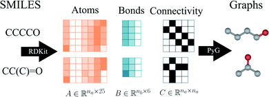 | ||
| Fig. 2 Schematic illustration of the construction of initial graphs from the solvent and solute SMILES. First, RDKit47 is used to extract the atom features, bond features and connectivity. Then, Pytorch Geometric (PyG)49 is employed to embed the corresponding matrices A and B into the graph with the connectivity described by matrix C. | ||
This way of representing molecules into graphs can be compared to other representation techniques of molecules, such as using a set of functional groups in group contribution methods. While the latter groups are defined manually using mostly chemical expert's knowledge, the former graph representation allows for methods such as GNNs to automatically optimize the binary-system fingerprint according to the structural information provided and its relative importance for predicting γij∞ (according to a provided error metric).
2.4 Graph neural network model
GNNs perform mathematical transformations over graph-structure data as input and return updated graphs as output (graph-to-graph). In this work, for each system there exist two molecular graphs (i.e., solvent and solute) that are mapped to a single γij∞ value. Two GNNs are used to process the molecular graphs of the solute and solvent species correspondingly (see Fig. 3a). For each convolutional layer l a graph with updated node features is obtained by using the following message passing scheme:48 | (1) |
![[Doublestruck R]](https://www.rsc.org/images/entities/char_e175.gif) d×d is a learnable weight matrix;
d×d is a learnable weight matrix; ![[scr N, script letter N]](https://www.rsc.org/images/entities/char_e52d.gif) (·) denotes the set of neighbouring nodes of a given node; ϕE(·) is a function mapping the edge feature vector between two nodes to an edge-conditioned weight matrix of size
(·) denotes the set of neighbouring nodes of a given node; ϕE(·) is a function mapping the edge feature vector between two nodes to an edge-conditioned weight matrix of size ![[Doublestruck R]](https://www.rsc.org/images/entities/char_e175.gif) d×d, which is implemented here as a single hidden-layer neural network with the ReLU activation function.
d×d, which is implemented here as a single hidden-layer neural network with the ReLU activation function.
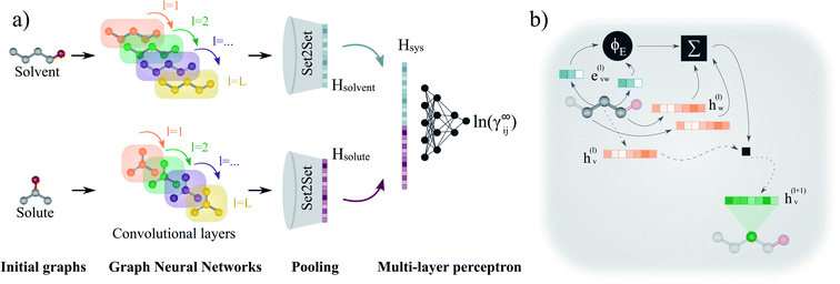 | ||
| Fig. 3 Schematic representation of the proposed GNN-based model for predicting ln(γij∞). (a) First, each molecular graph (i.e., solvent and solute) is passed through the corresponding graph neural network. Here, the node features of the graphs are updated at each layer l according to the message passing scheme described by eqn (1). After L convolutional layers, each node contains information of its L-level neighbourhood. Then, the final graphs are obtained by averaging the L graphs generated during the convolutions (jumping knowledge50). Afterwards, the molecular fingerprints are obtained from the global pooling layer Set2Set.51 Finally, the binary-system representation Hsys is obtained according to eqn 2, and a multi-layer perceptron maps it to the activity coefficient prediction. (b) Representation of the update performed to a node v (here, corresponding to the central carbon of 1-butanol) at convolution layer l. The neighbouring edge features evw(l) (blue vectors) are transformed by the multi-layer perceptron ϕE to perform the dot product with the embeddings of the neighbouring nodes hw(l). The previous embedding of node v is multiplied by matrix W and added to the neighbouring features transformation to obtain the new updated features vector hv(l+1) (green vector). | ||
Each convolutional layer l and its corresponding updated graphs are depicted with distinct colors in Fig. 3a. The operations involved in the message passing scheme (eqn (1)) are represented in Fig. 3b for the central node of the molecular graph. First, the vectors evw(l) representing the two chemical bonds connecting the central node are passed through the function ϕE(·) and are combined with the neighbouring node vectors hw(l) using the sum function. This “neighbourhood message” is then added to a linear transformation of the node hv(l) in which the message passing is being performed. The resulting vector hv(l+1) defines the representation of the central node for the updated graph in the next layer (depicted in green in Fig. 3b).
After L convolutional layers, L updated graphs have been generated. While some approaches only use the last updated graph to withdraw the final molecular representation,42,48 it has been shown that using the information contained in the progressive L updated graphs benefits the predictions of the GNN.50 This concept is known as “jumping knowledge”. In this work, the final graph is obtained by taking the mean of the L updated graphs. Then, this final graph is passed through a Set2Set51 global pooling layer that returns a single vector, representing the corresponding molecular species (i.e., the molecular fingerprint). This pooling model is invariant to permutation, and possesses more expressive power than the simple sum or average pooling.48 Then, after the molecular fingerprint of the solute Hsolute and solvent Hsolvent are obtained, these are concatenated into a single vector Hsys, which can be interpreted as the binary-system fingerprint,
| Hsys = Hsolvent‖Hsolute | (2) |
The key advantage of this approach is that the complete framework can be trained as an end-to-end system using backpropagation according to a specified error metric. This allows for the GNN-based model to select relevant features at the level of the solute and solvent fingerprints via the graph convolutional operations (potentially related to the molecular-shape contribution to nonideality), and to learn the important solvent–solute interactions using the binary-system fingerprint via the final multi-layer perceptron (potentially related to the contribution of intermolecular interactions to nonideality). This is in contrast to the manual selection of groups and the empirical determination of binary group-interaction parameters that characterize most successful group contribution methods.11,30–32 This is a cumbersome task that has been performed by only a few experts in the area for decades.
2.5 Training and validation
We randomly split the dataset into 80% for training and 20% for testing the model. Out of the training dataset, 90% was actually used for directly training the model, while the remaining 10% was used for validation and hyperparameter tuning. In contrast to other possible techniques for data splitting, such as molecular scaffold splitting,52 we decided to use random splits to focus more on the interpolation capabilities of the model. This is in contrast to studying the performance of the model while extrapolating to very dissimilar chemical structures. This follows the way in which most phenomenological models are used in practice, i.e., by using them according to their applicability domain. This is the same reason why several recommendations on the limitations and advantages of thermodynamic models are provided in the literature1,22 depending on the specific characteristics of the chemical system of interest (e.g., polar, aliphatic, aromatic). Fig. S1 in the ESI† shows that the composition densities of the train and test sets used in this work are similar with respect to each other according to the ranges of ln(γij∞) that they cover.The complete dataset involves only molecular solvents. Other chemical species, such as ionic liquids, were not included in the present study. However, the extension of the present methodology to ionic liquids would be straightforward if a proper database was used. We select the hyperparameters based on the model performance on the validation set, and report results on the test set unless otherwise stated. The model is implemented in Python 3.8 using PyTorch Geometric.49 To ease the training, we add a batch normalization layer53 and we use a dropout54 of 0.1 after each convolutional layer (eqn (1)) to prevent overfitting. The activation function Leaky ReLU was used after each layer (eqn (1)), with the exception of the last convolutional layer. The optimizer Adam55 was used to minimized the mean squared error (MSE) loss function using batches of 32 binary systems for 200 epochs. The learning rate is reduced if the validation error does not decrease (using a threshold of 10−4) for 3 consecutive epochs by a rate of 0.8. The optimal hyperparameters are obtained using Bayesian optimization and are explained in detail in the ESI.† All the experiments were performed on a single NVIDIA Tesla P100 GPU (16 GB).
2.6 Ensemble learning
In order to improve the accuracy of the predictions, a method of ensemble learning known as bagging56–58 was used. Here, 30 GNN-based models were trained independently using the same architecture and training hyperparameters and only varying the train/validation split randomly among them. The prediction is later obtained by averaging the independent predictions of the 30 models. This allows for the errors of the individual models to be averaged out, which (potentially) reduces the error of the ensemble. We have observed a significant reduction in the prediction error, which is expected given the relative small size of the data set considered. Similar behavior has been observed when applying this technique to similar-size molecular data sets.422.7 Parallel GNN hybrid model
Hybrid models refer to the combination of mechanistic and data-driven models. Combining these two has shown several advantages compared to the individual models in terms of accuracy, interpretability and complexity.59–61 Hybrid models can be arranged in series (i.e., when the prediction of one serves as the input to the other) or in parallel by coupling the independent predictions of the mechanistic and data-driven parts.59 Recently, a serial hybrid model for the prediction of activity coefficients at infinite dilution was developed,40 in which a Bayesian matrix completion method is combined with the UNIFAC-Dortmund model showing promising results. However, this method is still limited to the size of the matrix of experimental binary systems considered, and an extensive comparison with other phenomenological methods using an independent test set is still lacking. On the other side, the most common application of parallel hybrid models in chemical systems are the generation of residual models62–65 due to their flexibility in implementation. In this type of arrangement, a machine learning method is trained on the errors of the mechanistic model, and then their predictions are added up to reduce the overall error. This method is also known as boosting.66,67In this work, we have also studied the performance of parallel hybrid models by coupling our proposed GNN-based method to the considered 8 mechanistic models described in the introduction. This coupling is achieved by adding the residual predictions of the GNN to the predictions of the mechanistic model in order to obtained the final γij∞ prediction. The performance of these hybrid models have been compared to the purely mechanistic predictions and the purely GNN predictions achieving lower prediction errors in several cases. The architecture of the GNNs were kept the same as described in Section 2.4 for each of the 8 cases. However, this time our proposed GNN-based model, arranged as an ensemble of 30 independent GNN models, was trained on the residuals rij rather than in ln(γij∞) according to eqn (3).
| rij = ln(γij∞)exp − ln(γij∞)mech | (3) |
3 Results and discussion
3.1 GNN-based model predictions
The performance of the (single) GNN-based model, the ensemble of GNNs and the 8 mechanistic models is shown in Table 3. The performance scores were calculated based on the unscaled γi,j∞ values. A simple baseline is established with the Hildebrand model, which assumes that γij∞ can be accurately predicted by using only the evaporation enthalpy and the molar volume. The rest of the models perform much better and, with the exception of the HSP model, define the state-of-the-art in predicting γij∞ in practice. In Table 3, the confidence interval of the GNN single shows the standard deviation of each metric obtained by running 30 independent GNN models with different random train/validation splits for each run. The GNN ensemble model is obtained by averaging the prediction of the 30 individual GNN models. One essential difference between the GNN-based models and the mechanistic models is that, while the GNN can predict 100% of the data set, the other models are restricted to a smaller chemical space. For instance, the UNIFAC models can only be applied to the systems for which binary-interaction parameters for the involved UNIFAC groups are available. Similarly, empirical parameters for the other models are needed in order to make a prediction.22 This restricts the applicability domain of the model to the region defined by the available parameters, which explains their lower percentage coverage in Table 3. The only exception to this is COSMO-RS, the application coverage of which depends on the availability of the expensive DFT calculations on which this model is based on. For this study, only 97.2% of DFT simulations were available.| Model | Systems covered | MAE | SDEP | MSE | RMSE | R 2 | MAPE |
|---|---|---|---|---|---|---|---|
| Hildebrand | 54.66% | 2.55 × 10⁵ | 9.89 × 10⁶ | 9.79 × 10¹³ | 9.90 × 10⁶ | −7.92 × 10⁹ | 4.26 × 10⁵ |
| HSP | 56.23% | 16.03 | 122.37 | 15![[thin space (1/6-em)]](https://www.rsc.org/images/entities/char_2009.gif) ![[thin space (1/6-em)]](https://www.rsc.org/images/entities/char_2009.gif) 232.31 232.31 |
123.42 | −0.27 | 66.95 |
| UNIFAC (Ly) | 94.52% | 10.61 | 59.28 | 3626.24 | 60.22 | 0.56 | 32.99 |
| UNIFAC | 94.52% | 10.68 | 60.66 | 3794.03 | 61.60 | 0.54 | 32.37 |
| COSMO-RS | 97.22% | 10.78 | 67.18 | 4628.81 | 68.04 | 0.43 | 28.43 |
| UNIFAC (Do) | 94.91% | 8.54 | 56.82 | 3301.85 | 57.46 | 0.59 | 26.28 |
| Abraham | 44.27% | 4.18 | 33.58 | 1144.97 | 33.84 | 0.90 | 22.05 |
| MOSCED | 46.12% | 3.15 | 13.49 | 191.80 | 13.85 | 0.44 | 20.58 |
![[thin space (1/6-em)]](https://www.rsc.org/images/entities/char_2009.gif) |
|||||||
| GNN single (train) | 4.07 ± 0.57 | 31.06 ± 9.83 | 1077.93 ± 757.29 | 31.33 ± 9.82 | 0.88 ± 0.08 | 13.80 ± 0.52 | |
| GNN single (valid) | 3.83 ± 1.59 | 20.31 ± 11.90 | 571.35 ± 573.56 | 20.70 ± 11.96 | 0.89 ± 0.09 | 18.65 ± 2.69 | |
| GNN single (test) | 100% | 4.26 ± 0.60 | 29.60 ± 6.22 | 933.44 ± 419.07 | 29.91 ± 6.24 | 0.78 ± 0.1 | 25.27 ± 1.14 |
| GNN single (complete) | 4.09 ± 0.49 | 30.37 ± 8.32 | 1008.47 ± 610.84 | 30.65 ± 88.31 | 0.87 ± 0.08 | 16.48 ± 0.61 | |
![[thin space (1/6-em)]](https://www.rsc.org/images/entities/char_2009.gif) |
|||||||
| GNN ensemble (train/valid) | 3.48 | 25.79 | 677.18 | 26.02 | 0.92 | 12.19 | |
| GNN ensemble (test) | 100% | 3.91 | 26.73 | 729.69 | 27.01 | 0.82 | 22.66 |
| GNN ensemble (complete) | 3.57 | 25.98 | 687.68 | 26.22 | 0.91 | 14.29 | |
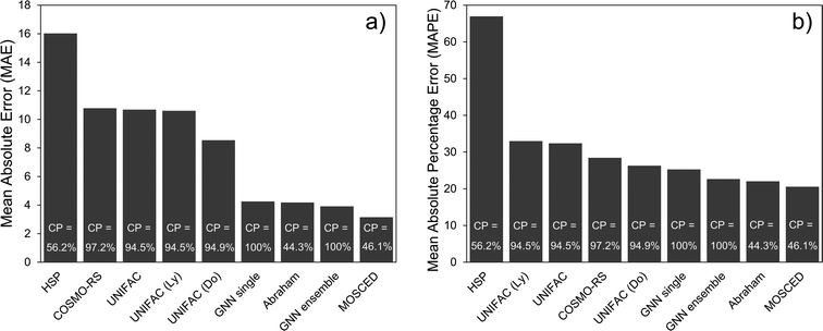
Given that different coverage of the whole data set is achieved by the different models (cf.Table 3), the comparison among them is difficult. While the performance results of the 8 mechanistic models are reported for their corresponding complete feasible dataset, the GNN results are reported for each of the train/validation/test splits. Also, the performance of the GNN models (trained only on the training set) on the complete dataset is reported for comparison. This is indicated with the word complete in Table 3. By considering the GNN results in the test set, the individual GNN model achieves a lower MAE than all the mechanistic models except for the specialized Abraham and MOSCED methods (cf.Fig. 4a). It is clear however, that precisely these two mechanistic models have a low coverage of predictable systems, 44.3% and 46.1% compared to the 100% of the GNN. This same behavior can be observed by looking only at the systems that can be predicted by the corresponding mechanistic model and are contained in the GNN test set (i.e., the intersection of feasible systems in the test set) as shown in Section S4.4 of the ESI.† Therefore, considering only the models that can cover more than 90% of the binary systems, the individual GNN outperforms them according to all the reported metrics. Nevertheless, the mean average percentage error (MAPE) of UNIFAC-Dortmund lays within one standard deviation of the individual GNN prediction (cf.Table 3). We can then conclude that according to the MAPE the individual GNN performs similar to the state-of-the art method UNIFAC-Dortmund. However, given that the MAE of the GNN is significantly better than UNIFAC-Dortmund, we can say that the GNN predicts highly non-ideal systems (where the absolute error is larger) better than UNIFAC-Dortmund. By contrast, if we consider the GNN ensemble model, this outperforms all the mechanistic models covering more than 90% of the data in all metrics, and even the Abraham model except in terms of R2 and MAPE (cf.Fig. 4a). A robustness study of the GNN predictions using a 5-fold cross validation is available in Section S4.7 of the ESI.†
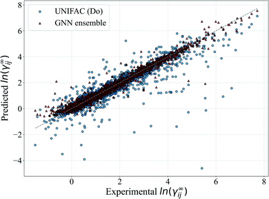
In Fig. 5, we show a comparison of the GNN ensemble method to the UNIFAC-Dortmund model in the form of a parity plot for all feasible systems. It can be seen that the GNN ensemble reduces the number of outliers considerably, and that the overall spread of the predictions from the perfect model (gray line) is much lower than the one achieved by UNIFAC-Dortmund. Comparison parity plots for all mechanistic models are available in Section S4.4 of the ESI† showing only feasible systems (for the corresponding mechanistic model) contained in the test set.
3.2 Hybrid GNN model
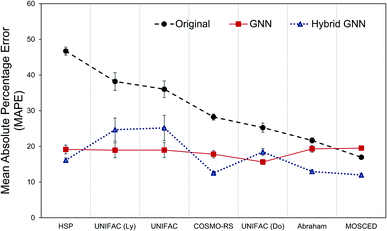
The question remains: should we simply forget about the mechanistic/phenomenological knowledge regarding γij∞ that has been acquired and proven its utility for decades and replace it with data-driven tools? Probably, a better approach would be to combine both methods in order to conserve the strengths of both, and potentially use machine learning as a tool to acquire new knowledge (hidden in the data but overseen in mechanistic approaches so far) that allows us to construct better mechanistic methods. A flexible approach to this was implemented in the form of parallel residual hybrid models for each one of the 8 mechanistic methods. These hybrid models were compared to the purely data-driven GNN ensemble. However, in order to have a fair comparison, we restricted the dataset available for training and testing of the GNN ensemble to the feasible data of each one of the 8 models.Fig. 6 shows the performance of all models (except the Hildebrand model baseline) according to their MAPE. The results are shown for the corresponding test data set only. It can be seen that the GNN performs significantly better that the mechanistic models when only the model's feasible data is considered. The exception to this is again for the specialized MOSCED method that has a low coverage of systems as discussed in Section 3.1. The hybrid GNN models further improve this performance in all cases except for the UNIFAC models. Similar behavior was encountered by the comparison between bagging and boosting models for UNIFAC-Dortmund using the matrix completion methodology.40 This demonstrates that, in general, by combining both mechanistic and data-driven models more reliable predictions are achieved. Another advantage of this approach is that the level of influence of the data-driven correction to the mechanistic model (mech) can be easily controlled by an applicability domain coefficient β introduced in eqn (4).
| ln(γij∞)pred = ln(γij∞)mech + βrij | (4) |
As pointed out by other works,68,69 the fact that the applicability domain is accessible during the predictions of data-driven models is of key importance for their application in the real-world.
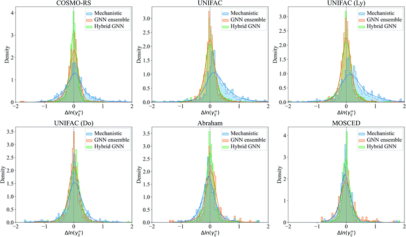
The prediction errors Δln(γij∞) = ln(γij∞)exp − ln(γij∞)pred of the mechanistic, GNN ensemble and hybrid GNN models are shown in Fig. 7 in the form of density plots. The Hildebrand and the HSP models are not shown here due to their poorer performance compared to the other mechanistic models and the evident superior performance of the GNN-based models when compared to these ones. It can be seen that the highest density of all models is centered close to the null-error. The only exception is the UNIFAC models, which present a clear deviation towards positive errors from the experimental activity coefficient values. The density of errors in the case of COSMO-RS improved considerably when using the combined hybrid GNN model. This behavior can possible be explained by the different sources of information that this model is using. On the one hand, the predicted charge density of the molecules and the intermolecular interactions are, in certain degree and according to theoretical foundations, embedded into the mechanistic part. On the other hand, the 2-dimensional structural information of the molecules and the interactions predicted from the binary-system fingerprint are included by the GNN model, acting as an effective data-based correction.
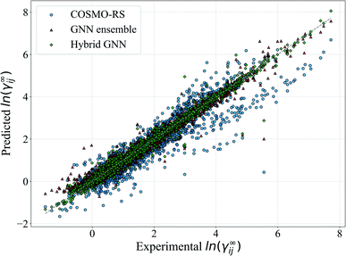
For illustration, the parity plot comparing COSMO-RS predictions to the GNN ensemble and the hybrid GNN is provided in Fig. 8. It can be seen that the hybrid approach has a lower distribution error across the range of γij∞ studied. This precise combination of two clearly different information sources is not present in the case of UNIFAC models with the same clarity. A possible reason for this is that both UNIFAC-based and GNN-based models are heavily relying on 2-dimensional structural information not complementing each other with a clear advantage. This connection between UNIFAC groups and the GNN convolutions has been already reported,42 especially in the context of higher-order GNNs.70 Comparison parity plots for all mechanistic models are available in Section S4.4 of the ESI† showing only systems contained in the test set.
4 Conclusions
The accurate prediction of physicochemical properties, including γij∞, is essential for the development of more efficient chemical processes. We have developed a predictive method based on graph neural networks (GNNs) that outperforms state-of-the-art methods such as UNIFAC-Dortmund and COSMO-RS (with respect to their mean absolute error (MAE) and mean average percentage error (MAPE)) in predicting γij∞ at 298.15 K. Since our framework is trained in an end-to-end fashion using backpropagation, our method can be extended whenever new data becomes available. Moreover, the 6 mechanistic models with the better performance, with which we compared our framework with, were hybridized by embedding a parallel residual GNN ensemble model that was trained on the errors of the corresponding method. We believe that such flexible hybrid models can be applied to enhance the prediction accuracy of well-known and vastly used thermodynamic models. This in turn will play a major role in the context of fully-automated experimentation facilities. We also believe that the use of such hybrid models can lead to a better understanding of the current weaknesses of mechanistic/phenomenological models (e.g., by doing attribution on the residual graphs). The GNN methodology can also be further extended to cover the temperature and composition dependency of the general activity coefficient γ. Moreover, how the graphs are constructed (e.g. functional group-based vs. atom-based) as well as the inclusion of global system features might have a substantial impact on the performance of the model for predicting γ. These aspects are kept here as future research questions.Data availability
The code for the training routines, the trained models and the results presented in this work can be found at https://github.com/edgarsmdn/GNN_IAC with DOI – 10.5281/zenodo.5690273. The version of the code employed for this study is version v1.0.0.Code availability
The model has been made publicly available at GitHub https://github.com/edgarsmdn/GNN_IAC along with the training routines and the experiments presented in this work.Author contributions
E. I. S. M. conceptualization, formal analysis, methodology, software and writing – original draft; S. L. conceptualization, resources and writing – review & editing; M. S. resources, supervision and writing – review & editing; K. S. funding acquisition, supervision and writing – review & editing.Conflicts of interest
There are no conflicts to declare.Acknowledgements
Edgar Ivan Sanchez Medina and Steffen Linke are also affiliated with the International Max Planck Research School for Advanced Methods in Process and Systems Engineering – IMPRS ProEng at the Max Planck Institute for Dynamics of Complex Technical Systems Magdeburg.References
- J. Gmehling, M. Kleiber, B. Kolbe and J. Rarey, Chemical Thermodynamics for Process Simulation, John Wiley & Sons, 2019 Search PubMed.
- C. S. Schacht, L. Zubeir, T. W. de Loos and J. Gross, Ind. Eng. Chem. Res., 2010, 49, 7646–7653 CrossRef CAS.
- T. Brouwer, S. R. Kersten, G. Bargeman and B. Schuur, Sep. Purif. Technol., 2021, 118727 CrossRef CAS.
- P. Harten, T. Martin, M. Gonzalez and D. Young, Environ. Prog. Sustainable Energy, 2020, 39, 13331 CrossRef CAS PubMed.
- S. Sandler, Fluid Phase Equilib., 1996, 116, 343–353 CrossRef CAS.
- J. H. Hildebrand, Chem. Rev., 1936, 18, 315–323 CrossRef CAS.
- C. M. Hansen, The Three Dimensional Solubility Parameter, Copenhagen Danish Technical Press, 1967, vol. 14 Search PubMed.
- E. R. Thomas and C. A. Eckert, Ind. Eng. Chem. Process Des. Dev., 1984, 23, 194–209 CrossRef CAS.
- A. Fredenslund, R. L. Jones and J. M. Prausnitz, AIChE J., 1975, 21, 1086–1099 CrossRef CAS.
- B. L. Larsen, P. Rasmussen and A. Fredenslund, Ind. Eng. Chem. Res., 1987, 26, 2274–2286 CrossRef CAS.
- U. Weidlich and J. Gmehling, Ind. Eng. Chem. Res., 1987, 26, 1372–1381 CrossRef CAS.
- M. H. Abraham, Chem. Soc. Rev., 1993, 22, 73–83 RSC.
- F. Eckert and A. Klamt, AIChE J., 2002, 48, 369–385 CrossRef CAS.
- B. E. Mitchell and P. C. Jurs, J. Chem. Inf. Comput. Sci., 1998, 38, 200–209 CrossRef CAS.
- F. Giralt, G. Espinosa, A. Arenas, J. Ferre-Gine, L. Amat, X. Girones, R. Carbó-Dorca and Y. Cohen, AIChE J., 2004, 50, 1315–1343 CrossRef CAS.
- E. Estrada, G. A. Díaz and E. J. Delgado, J. Comput.-Aided Mol. Des., 2006, 20, 539–548 CrossRef CAS PubMed.
- S. Ajmani, S. C. Rogers, M. H. Barley, A. N. Burgess and D. J. Livingstone, QSAR Comb. Sci., 2008, 27, 1346–1361 CrossRef CAS.
- K. Paduszynski, J. Chem. Inf. Model., 2016, 56, 1420–1437 CrossRef CAS PubMed.
- H. A. Behrooz and R. B. Boozarjomehry, Fluid Phase Equilib., 2017, 433, 174–183 CrossRef.
- G. Chen, Z. Song, Z. Qi and K. Sundmacher, AIChE J., 2021, 67, e17171 CAS.
- F. Jirasek, R. A. Alves, J. Damay, R. A. Vandermeulen, R. Bamler, M. Bortz, S. Mandt, M. Kloft and H. Hasse, J. Phys. Chem. Lett., 2020, 11, 981–985 CrossRef CAS PubMed.
- T. Brouwer and B. Schuur, Ind. Eng. Chem. Res., 2019, 58, 8903–8914 CrossRef CAS.
- T. Brouwer and B. Schuur, Green Chem., 2020, 22, 5369–5375 RSC.
- H. Benimam, C. S. Moussa, M. Hentabli, S. Hanini and M. Laidi, J. Chem. Eng. Data, 2020, 65, 3161–3172 CrossRef CAS.
- H. Benimam, C. Si-Moussa, M. Laidi and S. Hanini, Neural Comput. Appl., 2020, 32, 8635–8653 CrossRef.
- J. Gebhardt, M. Kiesel, S. Riniker and N. Hansen, J. Chem. Inf. Model., 2020, 60, 5319–5330 CrossRef CAS PubMed.
- P. J. Flory, J. Chem. Phys., 1942, 10, 51–61 CrossRef CAS.
- M. L. Huggins, J. Phys. Chem., 1942, 46, 151–158 CrossRef CAS.
- I. Kikic, P. Alessi, P. Rasmussen and A. Fredenslund, Can. J. Chem. Eng., 1980, 58, 253–258 CrossRef CAS.
- J. Gmehling, J. Li and M. Schiller, Ind. Eng. Chem. Res., 1993, 32, 178–193 CrossRef CAS.
- J. Gmehling, J. Lohmann, A. Jakob, J. Li and R. Joh, Ind. Eng. Chem. Res., 1998, 37, 4876–4882 CrossRef CAS.
- J. Gmehling, R. Wittig, J. Lohmann and R. Joh, Ind. Eng. Chem. Res., 2002, 41, 1678–1688 CrossRef CAS.
- J. L. Abboud, M. J. Kamlet and R. Taft, J. Am. Chem. Soc., 1977, 99, 8325–8327 CrossRef CAS.
- M. J. Kamlet, J. L. Abboud and R. Taft, J. Am. Chem. Soc., 1977, 99, 6027–6038 CrossRef CAS.
- M. J. Kamlet, P. W. Carr, R. Taft and M. H. Abraham, J. Am. Chem. Soc., 1981, 103, 6062–6066 CrossRef CAS.
- R. Taft, J.-L. M. Abboud and M. J. Kamlet, J. Am. Chem. Soc., 1981, 103, 1080–1086 CrossRef CAS.
- L. Sprunger, M. Clark, W. E. Acree and M. H. Abraham, J. Chem. Inf. Model., 2007, 47, 1123–1129 CrossRef CAS PubMed.
- C. C. Pye, T. Ziegler, E. Van Lenthe and J. N. Louwen, Can. J. Chem., 2009, 87, 790–797 CrossRef CAS.
- AMS 2021.1 COSMO-RS, SCM, Theoretical Chemistry, Vrije Universiteit, Amsterdam, The Netherlands, http://www.scm.com Search PubMed.
- F. Jirasek, R. Bamler and S. Mandt, Chem. Commun., 2020, 56, 12407–12410 RSC.
- J. Damay, F. Jirasek, M. Kloft, M. Bortz and H. Hasse, Ind. Eng. Chem. Res., 2021, 60, 14564–14578 CrossRef CAS.
- A. M. Schweidtmann, J. G. Rittig, A. König, M. Grohe, A. Mitsos and M. Dahmen, Energy Fuels, 2020, 34, 11395–11407 CrossRef CAS.
- M. Wen, S. M. Blau, E. W. C. Spotte-Smith, S. Dwaraknath and K. A. Persson, Chem. Sci., 2021, 12, 1858–1868 RSC.
- C. W. Coley, W. Jin, L. Rogers, T. F. Jamison, T. S. Jaakkola, W. H. Green, R. Barzilay and K. F. Jensen, Chem. Sci., 2019, 10, 370–377 RSC.
- K. Yang, K. Swanson, W. Jin, C. Coley, P. Eiden, H. Gao, A. Guzman-Perez, T. Hopper, B. Kelley, M. Mathea, A. Palmer, V. Settels, T. Jaakkola, K. Jensen and R. Barzilay, J. Chem. Inf. Model., 2019, 59, 3370–3388 CrossRef CAS PubMed.
- D. Weininger, J. Chem. Inf. Comput. Sci., 1988, 28, 31–36 CrossRef CAS.
- RDKit: Open-source cheminformatics, http://www.rdkit.org.
- J. Gilmer, S. S. Schoenholz, P. F. Riley, O. Vinyals and G. E. Dahl, International Conference on Machine Learning, 2017, pp. 1263–1272 Search PubMed.
- M. Fey and J. E. Lenssen, Fast graph representation learning with PyTorch Geometric, 2019 Search PubMed.
- K. Xu, C. Li, Y. Tian, T. Sonobe, K.-i. Kawarabayashi and S. Jegelka, International Conference on Machine Learning, 2018, pp. 5453–5462 Search PubMed.
- O. Vinyals, S. Bengio and M. Kudlur, Order Matters: Sequence to Sequence for Sets, 2015 Search PubMed.
- G. W. Bemis and M. A. Murcko, J. Med. Chem., 1996, 39, 2887–2893 CrossRef CAS PubMed.
- S. Ioffe and C. Szegedy, International Conference on Machine Learning, 2015, pp. 448–456 Search PubMed.
- N. Srivastava, G. Hinton, A. Krizhevsky, I. Sutskever and R. Salakhutdinov, J. Mach. Learn. Res., 2014, 15, 1929–1958 Search PubMed.
- D. P. Kingma and J. Ba, 2014, arXiv preprint arXiv:1412.6980.
- L. Breiman, Mach. Learn., 1996, 24, 123–140 Search PubMed.
- L. Breiman, Mach. Learn., 1996, 24, 49–64 Search PubMed.
- Y. Freund and R. E. Schapire, Experiments with a new boosting algorithm, International Conference on Machine Learning, Citeseer, 1996, vol. 96, pp. 148–156 Search PubMed.
- M. Von Stosch, R. Oliveira, J. Peres and S. F. de Azevedo, Comput. Chem. Eng., 2014, 60, 86–101 CrossRef CAS.
- J. Glassey and M. Von Stosch, Hybrid Modeling in Process Industries, CRC Press, 2018 Search PubMed.
- K. McBride, E. I. Sanchez Medina and K. Sundmacher, Chem. Ing. Tech., 2020, 92, 842–855 CrossRef CAS.
- M. Kamali and M. Mousavi, J. Supercrit. Fluids, 2008, 47, 168–173 CrossRef CAS.
- R. da Jia, Z.-z. Mao, Y.-q. Chang and L.-p. Zhao, Chem. Eng. Res. Des., 2011, 89, 722–728 CrossRef.
- M. W. Hermanto, R. D. Braatz and M.-S. Chiu, AIChE J., 2011, 57, 1008–1019 CrossRef CAS.
- E. A. del Rio Chanona, P. Petsagkourakis, E. Bradford, J. A. Graciano and B. Chachuat, Comput. Chem. Eng., 2021, 147, 107249 CrossRef.
- R. E. Schapire, Mach. Learn., 1990, 5, 197–227 Search PubMed.
- R. Meir and G. Rätsch, Advanced Lectures on Machine Learning, Springer, 2003, pp. 118–183 Search PubMed.
- B. Meredig, E. Antono, C. Church, M. Hutchinson, J. Ling, S. Paradiso, B. Blaiszik, I. Foster, B. Gibbons, J. Hattrick-Simpers, A. Matha and L. Ward, Mol. Syst. Des. Eng., 2018, 3, 819–825 RSC.
- A. Nigam, R. Pollice, M. F. Hurley, R. J. Hickman, M. Aldeghi, N. Yoshikawa, S. Chithrananda, V. A. Voelz and A. Aspuru-Guzik, Expert Opin. Drug Discovery, 2021, 1–15 Search PubMed.
- C. Morris, M. Ritzert, M. Fey, W. L. Hamilton, J. E. Lenssen, G. Rattan and M. Grohe, Proceedings of the AAAI Conference on Artificial Intelligence, 2019, pp. 4602–4609 Search PubMed.
Footnote |
| † Electronic supplementary information (ESI) available: Composition density of train/test data sets; hyperparameters tuning; performance metrics; data set description; additional results. See DOI: 10.1039/d1dd00037c |
| This journal is © The Royal Society of Chemistry 2022 |

