Microscopic origin of diffusive dynamics in the context of transition path time distributions for protein folding and unfolding
Received
11th July 2022
, Accepted 3rd October 2022
First published on 6th October 2022
Abstract
Experimentally measured transition path time distributions are usually analyzed theoretically in terms of a diffusion equation over a free energy barrier. It is though well understood that the free energy profile separating the folded and unfolded states of a protein is characterized as a transition through many stable micro-states which exist between the folded and unfolded states. Why is it then justified to model the transition path dynamics in terms of a diffusion equation, namely the Smoluchowski equation (SE)? In principle, van Kampen has shown that a nearest neighbor Markov chain of thermal jumps between neighboring microstates will lead in a continuum limit to the SE, such that the friction coefficient is proportional to the mean residence time in each micro-state. However, the practical question of how many microstates are needed to justify modeling the transition path dynamics in terms of an SE has not been addressed. This is a central topic of this paper where we compare numerical results for transition paths based on the diffusion equation on the one hand and the nearest neighbor Markov jump model on the other. Comparison of the transition path time distributions shows that one needs at least a few dozen microstates to obtain reasonable agreement between the two approaches. Using the Markov nearest neighbor model one also obtains good agreement with the experimentally measured transition path time distributions for a DNA hairpin and PrP protein. As found previously when using the diffusion equation, the Markov chain model used here also reproduces the experimentally measured long time tail and confirms that the transition path barrier height is ∼3kBT. This study indicates that in the future, when attempting to model experimentally measured transition path time distributions, one should perhaps prefer a nearest neighbor Markov model which is well defined also for rough energy landscapes. Such studies can also shed light on the minimal number of microstates needed to unravel the experimental data.
1 Introduction
The study of folding and unfolding dynamics of biomolecules has been a subject of long and sustained interest from the perspective of both theory1–5 and experiment.6–13 Folding and unfolding transitions are typically described as a barrier crossing process where the barrier is located between the two stable minima corresponding to the folded and unfolded molecules. The characteristic barrier height for such processes is typically greater than 10kBT with the result that the bio-molecules spend most of their time around the stable minima. Transitions between them are rare events and short lived, so that it is experimentally challenging to measure the transition path times as compared to the dwell times in one of the minima. Nonetheless, recent advances in single molecule experiments13–20 shed light on microscopic features of the transition path properties. These, in turn have triggered many theoretical studies.21–31 In most theoretical analyses, the dynamics is modeled in terms of a diffusion equation along a free energy surface connecting the stable states. The theoretical studies included a variety of dynamical effects, such as the role of memory23–25,27,29,30,32 inertial contributions,21,22 multidimensional transition paths28 and barrier shapes.33–37 However, none of these studies gave adequate agreement with the experimental data, which was accumulated using absorbing boundary conditions.
Our recent study of the transition path time distribution based on a diffusion equation (Smoluchowski equation) led to the conclusion that long time tails in the transition path time distribution indicate the existence of a “trap” in the transition path region.37 Introduction of a well along the transition path gave good agreement with the experimental data provided that the transition path barrier height is ∼3kBT, significantly higher than previous estimates of ∼1kBT based on theoretical studies using bell shaped free energy surfaces and open boundary conditions. The same study negated the requirement of multi-dimensional effects, free energy barrier asymmetry, sub-diffusive memory kernels or systematic ruggedness to explain the experimentally measured data.
Our present understanding of the experiments is predicated on the use of a Smoluchowski equation (SE) to describe the dynamics. This assumption needs proper clarification. It is well understood that the SE is a coarse-grained description of the barrier crossing process. It may be derived as the continuum limit of a nearest neighbor coupled set of master equations38,39 for motion through a series of uncorrelated transitions or random hopping between the many microstates that exist along the transition path. The “friction coefficient” used in the SE is related to the trapping time in the microstates. The strong friction limit, which validates the use of the SE, is a result of the long trapping times in the microstates. The free energy surfaces are known to be “rugged”39–43 and may be described in principle by a series of random well and barrier energies along the reaction path. A rugged energy landscape is more “physical” than that of the smooth free energy surface used in the diffusion equation analysis of the experiments. It is applicable not only to protein folding–unfolding40,41,44 but also to the glass transition.45,46 Zwanzig described the effect of the roughness of the potential by the introduction of random components on the potential energy surface.42 He found that the roughness of the potential leads to a non-Arrhenius increase in the mean first passage time and provided a relation for the dependence of the diffusion coefficient on the variance of the randomness associated with the rough potential. Bryngelson and Wolynes47 used a generalized master equation formalism and continuous-time random walk description to estimate mean first passage times for protein folding. They considered the number of native contacts as the reaction coordinate.48 Nevo et al.49 showed how the roughness can be measured by introducing an external force on the biosystem. In a series of studies Bagchi and co-workers investigated the role of spatial correlation of ruggedness and dimensionality dependence of diffusion and entropy when the energy landscape is rugged.50–52 In a recent study, Wales investigated how kinetic traps and corresponding barriers affect the first passage time distribution using a master equation approach.53 A similar analysis was also used in the study of single molecule enzyme kinetics.54
Li et al. studied the first-passage-time distribution in a time-dependent parabolic potential with spatial roughness using Kramers theory and a nonsingular integral equation.55,56 They concluded that the theory based on an integral equation almost correctly describes the mean first passage time for the whole range of external force whereas Kramers' theory57,58 is valid for only small external forces. Metzler and coworkers36 explored the role of roughness in the barrier by varying the amplitude and periodicity of the roughness to describe the transition path properties. In a recent experiment, Woodside and co-workers found brief pauses in transition paths, suggesting roughness or the presence of micro-barriers in the free energy landscape.59
Despite the wide usage of the diffusion equation, it is not at all clear why it is really valid in the context of protein folding and unfolding dynamics. The continuum limit of the nearest neighbor master equation is valid provided that the heights of the barriers separating the microstates change systematically. The continuum limit is not well defined when the free energy profile is that of a rough landscape. Even if the barrier profile is smooth it remains unclear how many microstates are need in practice to assure that the SE provides a valid description of the dynamics. These are the two central questions which motivated the present study. Theoretical formulation of the nearest neighbor master equation and the diffusion equation is reviewed in Section 2.1. We then provide in Section 2.2 a numerical study which compares the dynamics obtained by the two approaches. Specifically, we compare the transition path time distributions obtained for a bell shaped barrier profile for different models with different numbers of microstates. In Section 3 we apply the master equation model to analyse the experimentally measured transition path time distributions for the hairpin DNA molecule and the PrP protein.14,15 We find that also the master equation model leads to the conclusion that there is a central well along the reaction path which is responsible for the experimentally measured long time tails. We conclude with a discussion of the implications of the present work on the widespread usage of diffusion equations when modeling transition path time distributions for the folding–unfolding transition dynamics.
2 Diffusion and master equations
2.1 Theoretical framework
Experimentally, the transition path time is typically measured by considering the motion between two points along a suitably defined reaction coordinate leading from the folded to the unfolded states (and vice versa). The distribution of the times to cross the distance is the transition path time distribution. The two points are naturally chosen as half the difference of the full distance between the two stable states. After the system enters the transition path region for the first time, the distribution is obtained by noting the first time that the system then crosses the second point. This experimental definition of the transition path time distribution implies absorbing boundary conditions on the dynamics.
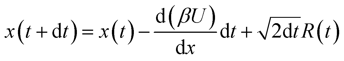
The diffusion equation, or equivalently the Langevin equation describing the motion along a one dimensional reaction coordinate ![[x with combining tilde]](https://www.rsc.org/images/entities/i_char_0078_0303.gif) is
is
| |  | (1) |
where,

is the force acting on the particle due to the free energy surface
U,

is a friction coefficient,
kB denotes Boltzmann's constant, and
F(
![[t with combining tilde]](https://www.rsc.org/images/entities/i_char_0074_0303.gif)
) is a Gaussian random force with zero mean and (Dirac) delta function correlation
| 〈F()〉 = 0 |
| | | 〈F()F(′)〉 = 2ζkBTδ( − ′) | (2) |
Numerical simulation of the dynamics is based on the following discretized and reduced diffusion equation
| |  | (3) |
where
x =
/
L is the reduced reaction coordinate, time is rescaled as
t =
D/
L2 with
D denoting the diffusion coefficient and 2
L denotes the experimental distance between the end points at −
L and
L. In order to compare with experiment (see Section 3), we consider
L = 2.5 nm and time is rescaled using the frequency factor 6 × 10
4 s
−1 for the DNA hairpin and 3 × 10
3 s
−1 for the PrP proteins.
14,37R(
t) is a Gaussian random number with zero mean and unit standard deviation. The stochastic differential equation is solved using the Euler–Maruyama method.
60
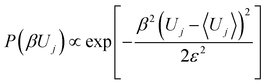
In the master equation formalism, the system gets trapped in different microstates from which it can escape to either side by an Arrhenius rate law. The location of the microwells is determined by discretizing the reaction coordinate x. The distances between the microwells is assumed to be l.
The distance between the wells is taken such that if there are N wells, the over all distance between the initial and final barrier is l(N + 1). As may be seen from ref. 38 and 39, that the continuum limit is obtained by letting l → 0 and n → ∞ such that the overall distance from right to left is kept fixed. The potential of mean force in the resulting diffusion equation is the profile of the barrier energies. Since we want to compare between the diffusion dynamics of a parabolic barrier obtained from the continuum limit of a master equation, we take the profile of the barrier heights to be that of a parabolic barrier, while the well depths have a Gaussian random component such that
| |  | (4) |
where,
β〈
Uj〉 is the mean well depth of all the wells taken to be −1 in all computations described below.
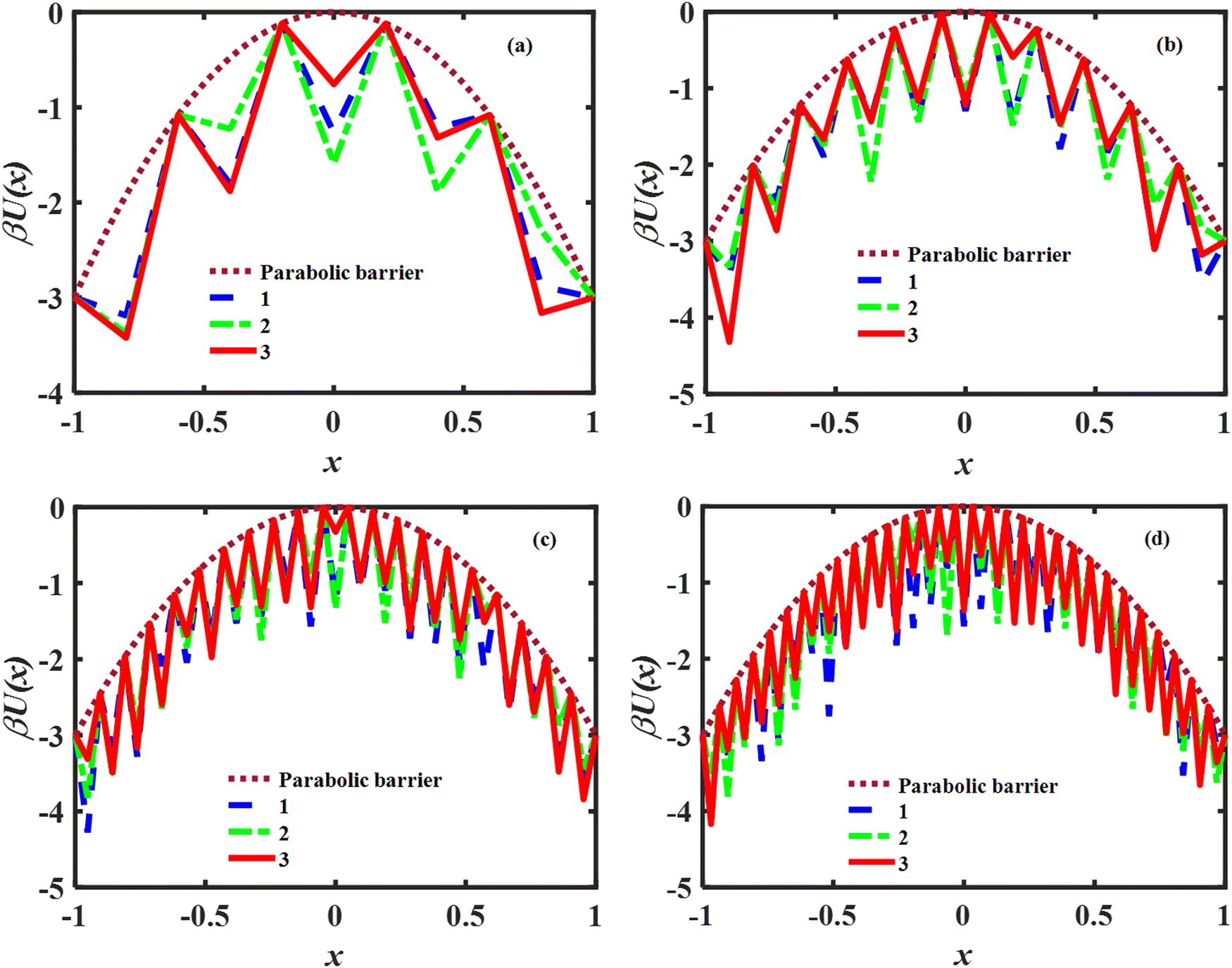
ε2 denotes the variance of the random part of the potential. The model barrier potentials used in this work are plotted in
Fig. 1 and consist of 5, 11, 21 and 31 microstates respectively. We used
ε = 0.3 for all the calculations. We note that the free energy profiles used throughout this work are continuous. The term “rugged” corresponds to the randomness of the well depths of the microstates. The concept of ruggedness in free energy landscapes is well established, as may be seen in some representative publications.
42,47–49,61–64
 |
| | Fig. 1 Plots of the discretized potential barriers and wells used in the numerical study of the master equation dynamics. Panels (a)–(d) show the profiles for 5, 11, 21 and 31 micro-wells respectively. The brown dotted line denotes the smooth parabolic barrier background. 1, 2 and 3 denote different realizations of stochastic well depths. Reduced units are used for the energies and distances. | |
To obtain the transition path time distribution from the diffusion equation, one needs to consider that the trajectories enter the transition region by crossing the left boundary located at −L and arrive at the right boundary L without returning to the left boundary. The transition path time distribution p(tTP) is then defined as
| | 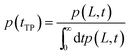 | (5) |
where,
p(
L,
t) is the numerically determined histogram of times with a bin width or equivalently a (reduced) time interval of Δ
t = 0.2. In all cases considered, the distribution decayed by the time
T = 10 so that 50 time bins were sufficient. It should be stressed, that any single trajectory was stopped the first time it reached the right boundary. The histogram is then taken for all transition path trajectories. The mean transition path time 〈
tTP〉 is defined as
| |  | (6) |
The calculation of the transition path time does not require a smooth potential when it is evaluated using the master equation. To obtain the transition path time distribution from the master equation, we use an algorithm based on the kinetic Monte Carlo simulation.65 The master equation approach is the same as the nearest neighbor jump model for a continuous time Markov chain where transitions from one state to another are governed through the forward and backward jump probabilities. The detailed steps are as follows. First, using the Arrhenius law, we evaluated the jump probability for going forward PF and backward PB from the j-th well
| |  | (7) |
where,
Uj±1/2 denotes the barrier height in either direction and
Uj is the well depth of the
jth micro-state. Then we generate a uniform random number
r1 ∈ [0,1]. If
r1 <
PF, a forward jump occurs, otherwise the jump is backwards. For the Markov process used, the waiting time distribution is exponential. The waiting time for the jump or escape from any one of the microstates was obtained by choosing a second random number
r2 ∈ [0,1] as
| |  | (8) |
where,
ktot =
kF +
kB. The forward (
kF) and backward (
kB) jump rates are defined as follows
| |  | (9) |
Here, the frequency prefactor
ν is taken to be a parameter in the theory, its magnitude is chosen such that the time scales agree with experiment.
We assume that initially at t = 0 the system is located at the j = 0 micro-state. We then impose absorbing boundary conditions at the j = 0 micro-state and at the j = N micro-state. The time is then advanced in steps of Δt and is stopped when the system reaches the final microstate. The histogram of final time values then gives the transition path time distribution with the condition of absorbing boundary at both ends.
2.2 Numerical results
The diffusion equation is solved by iterating eqn (3) with a reduced time step 10−3 for 106 trajectories imposing an absorbing boundary at the initial and final positions. Our earlier work37 indicated that the experimentally measured transition path barrier height is ∼3kBT so we use the same in our numerical studies presented in this paper. We will study the dynamics for a smooth reduced parabolic barrier| | | βU(x) = −βUTPx2; −1 ≤ x ≤ 1 | (10) |
where x = /L.
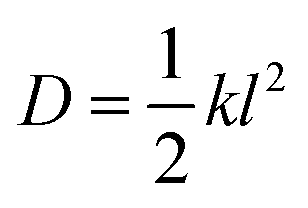
For the master equation dynamics the rate for the nearest neighbor jump is evaluated using eqn (10) where the value of the prefactors (ν) are chosen to take the (reduced) values of 18, 90, 320 and 700 for the models with 5, 11, 21 and 31 microstates, respectively. These prefactors assure that the magnitude of the mean transition path times obtained from both diffusion and master equation models are the same. They are obtained for each model using the relation between the diffusion coefficient (D) and the jump rate (k) for a one dimensional system random walk39,66
| |  | (11) |
where
l is the distance between the nearest neighbor microwells.
The barrier heights for each microstate model are taken so as to fit the parabolic barrier shape. However, as described above, the well depths are obtained from a Gaussian distribution with a mean well depth β〈Uj〉 = −1. As a result the average barrier height for the nearest neighbor jump is assumed to be 1.
The transition path time distribution obtained from the diffusion equation is compared with the results obtained from the master equation in Fig. 2. The brown dotted line shows the distribution obtained from the diffusion equation. In each panel, the solid red, dot-dash green and dashed blue lined show the transition path time distributions obtained from the master equation for three different realizations of the random wells. Panels (a)–(d) correspond to 5, 11, 21 and 31 microwells used in the master equations. Each distribution was obtained from 106 trajectories propagated for up to 3 × 10³ time steps. Comparison of the plots shows that the master equation distributions converge to the diffusion equation result as the number of microstates increases, irrespective of the precise realization of the random well depths. The resulting mean transition path times (see eqn (15)) are compared in Table 1. These mean time values show that although the mean time is roughly the same, it does change somewhat randomly, depending on the model used.
 |
| | Fig. 2 Comparison of the normalized (to unity) transition path time distributions found using the diffusion and master equations for different potential barrier models consisting different numbers of microwells 5, 11, 21 and 31 realizations. 1, 2 and 3 indicate different barrier realizatons. (a–d) Denote plots for different models with different prefactors for the rate of a jump (ν) (a) 5 microstates with ν = 18 (b) 11 microstates with ν = 90 (c) 21 microstates with ν = 320 (d) 31 microstates with ν = 700. | |
Table 1 Comparison of the mean transition path times obtained from the diffusion equation and master equation models presented in Fig. 1. Reduced units are used throughout
| Diffusion equation |
Master equation |
| 0.42 |
0.36 (1), 0.42 (2), 0.34 (3) (5 microstates) |
| 0.39 (1), 0.41 (2), 0.36 (3) (11 microstates) |
| 0.41 (1), 0.39 (2), 0.35 (3) (21 microstates) |
| 0.42 (1), 0.38 (2), 0.36 (3) (31 microstates) |
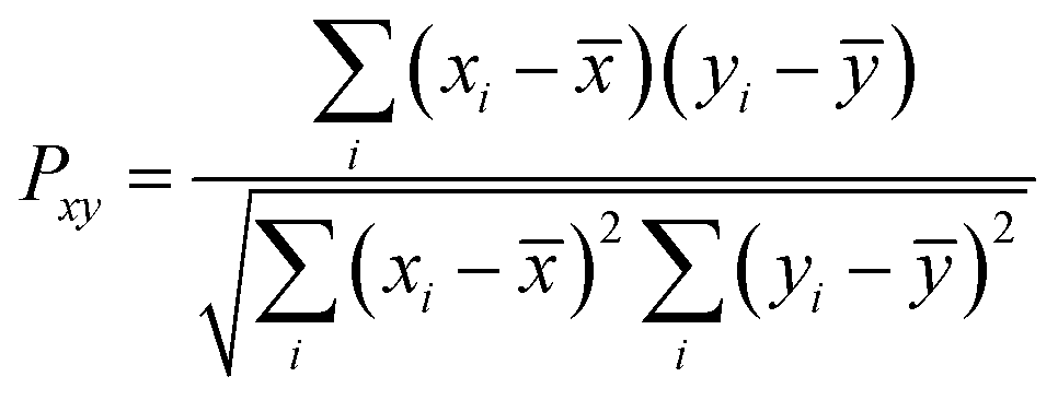
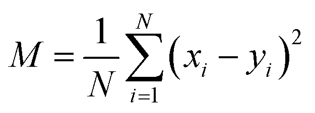
For a more quantitative comparison of the distributions we computed the Pearson correlation function and mean squared deviations of the master equation models with respect to the diffusion equation. The Pearson correlation function and mean squared error are defined as
| |  | (12) |
| |  | (13) |
where
xi and
yi denote two different data sets. If
Pxy = 1 and
M = 0, the two data sets are identical. The quality of fitting is examined for the best fit results obtained from the different runs shown in
Fig. 1 using master equation dynamics.
The resulting quality of fit is provided in Table 2. The fitting parameter is calculated only for the best fits obtained from different realizations of random microstate well depths in the models. As noted qualitatively from Fig. 1, it is evident from Table 2 that the correlation between data sets increases and the mean squared error decreases as the number of microstates increases. The trend suggests the validation of the diffusion equation as a model for the transition path dynamics, provided that one may assume a sufficient number of microstates bridging the path from the unfolded to the folded states. When the number of microstates is greater than 20 the quality of the fitting coefficients is almost unity and remains unchanged.
Table 2 Comparison of fitting coefficients for transition path time distributions obtained with the diffusion and master equations
| No. of microstates |
PCC(Pxy) |
MSE(M) |
| 5 |
0.92 |
0.13 |
| 11 |
0.96 |
0.06 |
| 21 |
0.98 |
0.03 |
| 31 |
0.98 |
0.03 |
3 Fitting the experimentally measured data with master equation modeling
In our earlier study, we showed that when analyzing the experimentally measured transition path time distribution using the SE and absorbing boundary conditions one observes a long time tail. We found that a simple bell shaped potential of mean force cannot account for it. It was necessary to add a potential well around the barrier top. This well served as a “trap” accounting for the long time tail.37 Here we will show that good agreement with experiment is obtained also when the dynamics is governed by the master equation.
For the diffusion equation solution a piecewise continuous potential is constructed. For the DNA hairpin the parameters are taken to assure the measured activation energy of ∼10kBT. The potential chosen is:
Region-I
| | | 8.1(x + 2)4 − 9.1; −3 ≤ x ≤ −1 | (14) |
Region-II
| | | −92.571(x + 0.825)2 + 1.835; −1 ≤ x ≤ −0.795 | (15) |
Region-III
| | | 3.493x2 − 0.456; −0.795 ≤ x ≤ 0.795 | (16) |
Region-IV
| | | −92.571(x − 0.825)2 + 1.835; 0.795 ≤ x ≤ 1 | (17) |
Region-V
| | | 8.1(x − 2)4 − 9.1; 1 ≤ x ≤ 3 | (18) |
A similar piece-wise continuous potential is constructed for the PrP protein. Here, the Arrhenius activation energy is ∼5kBT and the potential is.
Region-I
| | | 3.4(x + 2)6 − 4.4; −3 ≤ x ≤ −1 | (19) |
Region-II
| | | −40.8(x + 0.75)2 + 1.55; −1 ≤ x ≤ −0.68 | (20) |
Region-III
| | | 4.2x2 − 0.592; −0.68 ≤ x ≤ 0.68 | (21) |
Region-IV
| | | −40.8(x − 0.75)2 + 1.55; 0.68 ≤ x ≤ 1 | (22) |
Region-V similarly, on the right side of region-III (
eqn (20)) is
| | | 3.4(x − 2)6 − 4.4; 1 ≤ x ≤ 3. | (23) |
These two potentials are plotted in
Fig. 3. The parameters related to the equations for the free energy for both proteins are obtained using the fact that the transition path covers half of the distance between the folded and unfolded minima. Assuming that the start and end points of the transition region are ±1 and using the known experimental activation energy, one can readily determine region I of the potential. Parameters for regions II and III are obtained using the conditions of continuity of the potential and its derivative. The well depth in the central region is chosen such that the mean transition path time would agree with the known experimental time. As the potential is symmetric the parameters for regions IV and V are the same as regions II and I respectively.
 |
| | Fig. 3 Model potential energy surfaces for the DNA hairpin and PrP protein. The transition path covers half of the distance between the minima of the folded and unfolded states. The transition path region is extended to obtain a full potential energy surface where the barrier height is fitted to the experimental estimate.14 | |
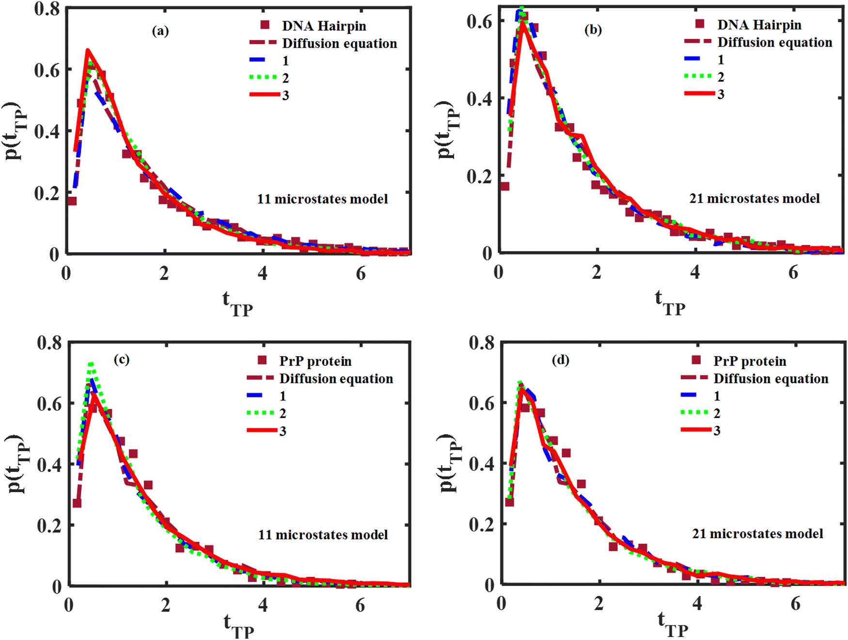
To apply the master equation modelling, the potentials are discretized using either 11 or 21 microstates keeping the potential energy profile defined by the potentials shown in Fig. 3. The resulting surfaces are shown in Fig. 4. The upper two panels show the microstate structure used for the DNA hairpin with 11 and 21 wells. As in Fig. 1 we employed three different random realizations of the profile of the microstates, these are shown as the solid (red) line, dotted (green) line and dashed (blue) line. The same is shown for the PrP protein in the bottom two panels of the figure.
 |
| | Fig. 4 Microstate profile of the potentials used to simulate the experimentally measured transition path time distributions. For further explanations, see the text. | |
One may well ask how does one determine the number of microstates needed for a given system. The method we are suggesting, which is based on knowledge of the experimental time distributions is as follows. One initiates the fit with a small number of microstates of the order of 3–5, choosing an odd number of microstates to maintain symmetry. One then must ascertain whether the experimental mean time agrees with the model as well as use quantitative measures such as the Pearson correlation coefficient (PCC) and mean squared error (MSE) to assure that the simulation gives good agreement with the measured time distribution. As the number of microstates is increased, one will find that the fitting measures saturate. The number of microstates needed to simulate the experiment is the number needed to reach the saturation region. Inspection of Table 1 shows that in the cases studied here, 21 microstates are needed for the quantitative description of the transition path time distribution.
A comparison between the theoretical transition path time distributions obtained from the diffusion and master equations with the experimentally measured distributions for the DNA hairpin and PrP protein molecules is shown in Fig. 5. The experimental distributions are adapted from ref. 14 and normalized to unit area, as are the theoretical distributions shown in the figure. The time scale is reduced, using the experimentally fitted frequency factor 6 × 10⁴ s−1 for the DNA hairpin and 3 × 10³ s−1 for the PrP protein. The frequency factor ν is chosen as ν = 90 for the 11 microstates model, while ν = 320 is chosen when using 21 microstates. The solid (red), dotted (green) and dashed (blue) lines are for the three different realizations of the microwells, shown in Fig. 4.
 |
| | Fig. 5 Comparison between experimental and theoretical (diffusion and Master equations) normalized transition path time distributions. Panels (a and b) show the comparison for the DNA hairpin using 11 and 21 microstates respectively. Panels (c and d) show the same for the PrP protein. | |
As may be observed in all panels of the figure, good agreement between theory and experiment is obtained, irrespective of the theoretical model used. As few as 11 microstates are sufficient to account for the measured distributions. These results further validate the need to include a trap in the transition path region that leads to the long time tail in the time distribution. In this context, following our work, Woodside and co-workers recently observed brief pauses in the transition paths, indicating the existence of ruggedness or traps in the transition region, negating models based on a simple barrier free energy profile.59 These results further verify our claim that the transition path barrier height is ∼3kBT barrier height37 rather than ∼1kBT as found in ref. 14. We believe that our result is realistic, especially when keeping in mind that the activation energy for the folding–unfolding transition is of the order of ∼10kBT while the transition path begins and ends at half the distance between the minima of the folded and unfolded bio-molecules.
The respective mean (reduced) transition times obtained from the diffusion and master equations are compared with experiment in Table 3 using the diffusion equation and the three different realizations of the microstates, as shown in Fig. 4. As may be seen from the table, the agreement between theory and experiment is reasonable, for all models considered, although it improves when using 21 microstates instead of 11.
Table 3 Comparison of experimental and theoretical mean transition path times for the DNA hairpin and PrP protein. Further explanations are given in the text
|
|
Experiment |
Diffusion equation |
Master equation |
| DNA hairpin |
1.62 ± 0.12 |
1.69 |
1.73(1), 1.54(2), 1.47(3) (11 microstates) |
| 1.51(1), 1.68(2), 1.69(3) (21 microstates) |
| PrP protein |
1.50 ± 0.30 |
1.53 |
1.46(1), 1.34(2), 1.57(3) (11 microstates) |
| 1.51(1), 1.45(2), 1.50(3) (21 microstates) |
4 Discussion
The most common framework used to analyze bio-molecular folding and unfolding processes is the diffusion equation. Many theoretical studies have used a Smoluchowski equation in the presence of a potential barrier to describe transition path properties. The major thrust of the present work was to obtain insight as to why a diffusion equation is at all a valid tool. Why is it justified on a more microscopic level? What is the microscopic source of friction which governs the diffusion dynamics?
It is well accepted that the free energy landscape along the reaction path is not “smooth” but rugged with many microstates along the way. To account for this we presented results based on numerical solution of a master equation for the nearest neighbor hopping transition between microstates in the presence of absorbing boundary condition. In this picture, the friction comes from the mean residence time of the system in each of the microstates before escaping them. The mean residence time is long as compared to internal motion within a bio-molecule, leading to diffusive like dynamics as evidenced by comparison with a suitably chosen diffusion equation.
The comparison between transition path time distributions obtained using the diffusion and master equation dynamics shows that agreement increases with the number of microstates. One can obtain quite good agreement between mean transition times even for less than ten microstates, however inspection of the transition path time distribution shows that typically one would need two dozen microstates to obtain similar results. On the other hand, analysis of experimentally measured transition path time distributions showed that one can mimic the experimental results using as few as 11 microstates. This comparison also further validates our recent conclusion that the long time tail found in the experimental distribution indicates the existence of an intermediate well along the reaction path whose well depth is a few kBT. The master equation simulation also confirms that the transition path barrier is ∼3kBT height as also obtained from an analysis based on the diffusion equation.37
The present study suggests that in principle, there is no need to use the simplistic diffusion equation dynamics to analyze transition path time distributions. A master equation approach, which is arguably more realistic due to the rugged energy landscape inherent to it, may lead not only to similar conclusions, but may also provide more insight as to the dynamics. For example, the well needed to obtain agreement with the long time tail experimental data itself is not “smooth” as in the diffusion equation, but contains a number of microstates along it, as may be discerned from Fig. 4.
On the other hand, the diffusion equation has the distinct advantage that sometimes, as with a parabolic21 or cusped barrier the solution is analytic.33,34 The fact that the master equation dynamics may lead to diffusion dynamics provides some justification for employing such analytic models, which shed light on the diffusional dynamics.
Finally, we do note that also the Markov modelling presented in this paper is an idealised description of the transition between folded and unfolded conformations of bio-molecules. Perhaps the present study provides further impetus for molecular dynamics studies on “realistic” force fields which include all molecular degrees of freedom.23,67,68 These may then be compared with Markov and diffusion equation studies.
Author contributions
RD contributed to the relevant theoretical developments, implemented the computational work and was an equal contributor to the writing up of the manuscript. EP suggested the topic, contributed to the theory and was an equal contributor to the writing up of the manuscript.
Conflicts of interest
There are no conflicts to declare.
Acknowledgements
This work has been generously supported by a grant of the Israel Science Foundation.
References
- G. Hummer, J. Chem. Phys., 2004, 120, 516–523 CrossRef CAS PubMed.
- A. Berezhkovskii and A. Szabo, J. Chem. Phys., 2005, 122, 014503 CrossRef PubMed.
- B. W. Zhang, D. Jasnow and D. M. Zuckerman, J. Chem. Phys., 2010, 132, 054107 CrossRef PubMed.
- S. Chaudhury and D. E. Makarov, J. Chem. Phys., 2010, 133, 034118 CrossRef PubMed.
- W. K. Kim and R. R. Netz, J. Chem. Phys., 2015, 143, 224108 CrossRef PubMed.
- E. Rhoades, M. Cohen, B. Schuler and G. Haran, J. Am. Chem. Soc., 2004, 126, 14686–14687 CrossRef CAS PubMed.
- H. S. Chung, J. M. Louis and W. A. Eaton, Proc. Nat. Acad. Sci. U. S. A., 2009, 106, 11837–11844 CrossRef CAS PubMed.
- H. S. Chung, K. McHale, J. M. Louis and W. A. Eaton, Science, 2012, 335, 981–984 CrossRef CAS PubMed.
- K. Neupane, D. B. Ritchie, H. Yu, D. A. Foster, F. Wang and M. T. Woodside, Phys. Rev. Lett., 2012, 109, 068102 CrossRef PubMed.
- H. Yu, A. N. Gupta, X. Liu, K. Neupane, A. M. Brigley, I. Sosova and M. T. Woodside, Proc. Nat. Acad. Sci. U. S. A., 2012, 109, 14452–14457 CrossRef CAS PubMed.
- H. Yu, D. R. Dee, X. Liu, A. M. Brigley, I. Sosova and M. T. Woodside, Proc. Nat. Acad. Sci. U. S. A., 2015, 112, 8308–8313 CrossRef CAS PubMed.
- H. S. Chung, S. Piana-Agostinetti, D. E. Shaw and W. A. Eaton, Science, 2015, 349, 1504–1510 CrossRef CAS PubMed.
- P. Tripathi, A. Firouzbakht, M. Gruebele and M. Wanunu, J. Phys. Chem. Lett., 2022, 13, 5918–5924 CrossRef CAS PubMed.
- K. Neupane, D. A. Foster, D. R. Dee, H. Yu, F. Wang and M. T. Woodside, Science, 2016, 352, 239–242 CrossRef CAS PubMed.
- K. Neupane, F. Wang and M. T. Woodside, Proc. Nat. Acad. Sci. U. S. A., 2017, 114, 1329–1334 CrossRef CAS PubMed.
- K. Neupane, N. Q. Hoffer and M. Woodside, Phys. Rev. Lett., 2018, 121, 018102 CrossRef CAS PubMed.
- H. S. Chung and W. A. Eaton, Curr. Opin. Struct. Biol., 2018, 48, 30–39 CrossRef CAS PubMed.
- N. Q. Hoffer, K. Neupane, A. G. Pyo and M. T. Woodside, Proc. Nat. Acad. Sci. U. S. A., 2019, 116, 8125–8130 CrossRef CAS PubMed.
- F. Sturzenegger, F. Zosel, E. D. Holmstrom, K. J. Buholzer, D. E. Makarov, D. Nettels and B. Schuler, Nat. Commun., 2018, 9, 1–11 CrossRef CAS PubMed.
- A. Mehlich, J. Fang, B. Pelz, H. Li and J. Stigler, Front. Chem., 2020, 8, 587824 CrossRef CAS PubMed.
- E. Pollak, Phys. Chem. Chem. Phys., 2016, 18, 28872–28882 RSC.
- M. Laleman, E. Carlon and H. Orland, J. Chem. Phys., 2017, 147, 214103 CrossRef CAS PubMed.
- R. Satija, A. Das and D. E. Makarov, J. Chem. Phys., 2017, 147, 152707 CrossRef PubMed.
- E. Medina, R. Satija and D. E. Makarov, J. Phys. Chem. B, 2018, 122, 11400–11413 CrossRef CAS PubMed.
- E. Carlon, H. Orland, T. Sakaue and C. Vanderzande, J. Phys. Chem. B, 2018, 122, 11186–11194 CrossRef CAS PubMed.
- P. Cossio, G. Hummer and A. Szabo, J. Chem. Phys., 2018, 148, 123309 CrossRef PubMed.
- R. Satija and D. E. Makarov, J. Phys. Chem. B, 2019, 123, 802–810 CrossRef CAS PubMed.
- R. Satija, A. M. Berezhkovskii and D. E. Makarov, Proc. Nat. Acad. Sci. U. S. A., 2020, 117, 27116–27123 CrossRef CAS PubMed.
- D. Singh, K. Mondal and S. Chaudhury, J. Phys. Chem. B, 2021, 125, 4536–4545 CrossRef CAS PubMed.
- V. Singh and P. Biswas, J. Stat. Mech., 2021, 2021, 063502 CrossRef.
- N. Mothi and V. Munoz, J. Phys. Chem. B, 2021, 125, 12413–12425 CrossRef CAS PubMed.
- C. Ayaz, L. Tepper, F. N. Brünig, J. Kappler, J. O. Daldrop and R. R. Netz, Proc. Nat. Acad. Sci. U. S. A., 2021, 118, e2023856118 CrossRef CAS PubMed.
- A. M. Berezhkovskii, L. Dagdug and S. M. Bezrukov, J. Phys. Chem. B, 2017, 121, 5455–5460 CrossRef CAS PubMed.
- A. M. Berezhkovskii, L. Dagdug and S. M. Bezrukov, J. Phys. Chem. B, 2019, 123, 3786–3796 CrossRef CAS PubMed.
- M. Caraglio, T. Sakaue and E. Carlon, Phys. Chem. Chem. Phys., 2020, 22, 3512–3519 RSC.
- H. Li, Y. Xu, Y. Li and R. Metzler, Eur. Phys. J. Plus, 2020, 135, 1–22 CrossRef.
- R. Dutta and E. Pollak, Phys. Chem. Chem. Phys., 2021, 23, 23787–23795 RSC.
-
N. G. Van Kampen, Stochastic processes in physics and chemistry, Elsevier, 1992, vol. 1 Search PubMed.
- E. Pollak, A. Auerbach and P. Talkner, Biophys. J., 2008, 95, 4258–4265 CrossRef CAS PubMed.
- A. Ansari, J. Berendzen, S. F. Bowne, H. Frauenfelder, I. Iben, T. B. Sauke, E. Shyamsunder and R. D. Young, Proc. Nat. Acad. Sci. U. S. A., 1985, 82, 5000–5004 CrossRef CAS PubMed.
- H. Frauenfelder, F. Parak and R. D. Young, Ann. Rev. Biophys. Biophys. Chem., 1988, 17, 451–479 CrossRef CAS PubMed.
- R. Zwanzig, Proc. Nat. Acad. Sci. U. S. A., 1988, 85, 2029–2030 CrossRef CAS PubMed.
- H. Frauenfelder, S. G. Sligar and P. G. Wolynes, Science, 1991, 254, 1598–1603 CrossRef CAS PubMed.
- J. Wang, J. Onuchic and P. Wolynes, Phys. Rev. Lett., 1996, 76, 4861 CrossRef CAS PubMed.
- P. Scheidler, W. Kob and K. Binder, J. Phys. Chem. B, 2004, 108, 6673–6686 CrossRef CAS.
- T. Chow, Phys. Lett. A, 2005, 342, 148–155 CrossRef CAS.
- J. D. Bryngelson and P. G. Wolynes, J. Phys. Chem., 1989, 93, 6902–6915 CrossRef CAS.
- C. Hyeon and D. Thirumalai, Proc. Nat. Acad. Sci. U. S. A., 2003, 100, 10249–10253 CrossRef CAS PubMed.
- R. Nevo, V. Brumfeld, R. Kapon, P. Hinterdorfer and Z. Reich, EMBO Rep., 2005, 6, 482–486 CrossRef CAS PubMed.
- S. Banerjee, R. Biswas, K. Seki and B. Bagchi, J. Chem. Phys., 2014, 141, 09B617 CrossRef PubMed.
- K. Seki and B. Bagchi, J. Chem. Phys., 2015, 143, 194110 CrossRef PubMed.
- K. Seki, K. Bagchi and B. Bagchi, J. Chem. Phys., 2016, 144, 194106 CrossRef PubMed.
- D. J. Wales, J. Phys. Chem. Lett., 2022, 13, 6349–6358 CrossRef CAS PubMed.
- J. Cao and R. J. Silbey, J. Phys. Chem. B, 2008, 112, 12867–12880 CrossRef CAS PubMed.
- Y. Li, Y. Xu and J. Kurths, Phys. Rev. E, 2019, 99, 052203 CrossRef CAS PubMed.
- Y. Li, Y. Xu, J. Kurths and J. Duan, Chaos, 2019, 29, 101102 CrossRef PubMed.
- G. Hummer and A. Szabo, Biophys. J., 2003, 85, 5–15 CrossRef CAS.
- O. K. Dudko, G. Hummer and A. Szabo, Phys. Rev. Lett., 2006, 96, 108101 CrossRef PubMed.
- N. Q. Hoffer, K. Neupane and M. T. Woodside, Proc. Nat. Acad. Sci. U. S. A., 2021, 118, e2101006118 CrossRef CAS PubMed.
- D. J. Higham, SIAM Rev., 2001, 43, 525–546 CrossRef.
- P. G. Wolynes, J. N. Onuchic and D. Thirumalai, Science, 1995, 267, 1619–1620 CrossRef CAS PubMed.
- J. N. Onuchic, P. G. Wolynes, Z. Luthey-Schulten and N. D. Socci, Proc. Nat. Acad. Sci. U. S. A., 1995, 92, 3626–3630 CrossRef CAS PubMed.
-
W. Janke, Rugged Free Energy Landscapes, Springer, 2008, pp. 1–7 Search PubMed.
- R. Moulick, R. R. Goluguri and J. B. Udgaonkar, J. Mol. Biol., 2019, 431, 807–824 CrossRef CAS PubMed.
- A. B. Bortz, M. H. Kalos and J. L. Lebowitz, J. Comp. Phys., 1975, 17, 10–18 CrossRef.
- S. Chandrasekhar, Rev. Mod. Phys., 1943, 15, 1 CrossRef.
- T. Mori and S. Saito, J. Phys. Chem. B, 2016, 120, 11683–11691 CrossRef CAS PubMed.
- S. Sharma, V. Singh and P. Biswas, ACS Phys. Chem. Au, 2022, 2, 353–363 CrossRef CAS.
|
| This journal is © the Owner Societies 2022 |
Click here to see how this site uses Cookies. View our privacy policy here. 
 Open Access Article
 This Open Access Article is licensed under a Creative Commons Attribution-Non Commercial 3.0 Unported Licence
 *
*

 is the force acting on the particle due to the free energy surface U,
  is a friction coefficient, kB denotes Boltzmann's constant, and F(