
 Open Access Article
 This Open Access Article is licensed under a
 Creative Commons Attribution 3.0 Unported Licence
DFT exchange: sharing perspectives on the workhorse of quantum chemistry and materials science
Andrew M.
Teale
 *a,
Trygve
Helgaker
*b,
Andreas
Savin
*c,
Carlo
Adamo
d,
Bálint
Aradi
e,
Alexei V.
Arbuznikov
f,
Paul W.
Ayers
g,
Evert Jan
Baerends
h,
Vincenzo
Barone
i,
Patrizia
Calaminici
j,
Eric
Cancès
k,
Emily A.
Carter
l,
Pratim Kumar
Chattaraj
m,
Henry
Chermette
n,
Ilaria
Ciofini
d,
T. Daniel
Crawford
op,
Frank
De Proft
q,
John F.
Dobson
r,
Claudia
Draxl
st,
Thomas
Frauenheim
euv,
Emmanuel
Fromager
w,
Patricio
Fuentealba
x,
Laura
Gagliardi
y,
Giulia
Galli
z,
Jiali
Gao
aaab,
Paul
Geerlings
q,
Nikitas
Gidopoulos
ac,
Peter M. W.
Gill
ad,
Paola
Gori-Giorgi
ae,
Andreas
Görling
af,
Tim
Gould
ag,
Stefan
Grimme
ah,
Oleg
Gritsenko
ae,
Hans Jørgen Aagaard
Jensen
ai,
Erin R.
Johnson
aj,
Robert O.
Jones
ak,
Martin
Kaupp
f,
Andreas M.
Köster
j,
Leeor
Kronik
al,
Anna I.
Krylov
am,
Simen
Kvaal
b,
Andre
Laestadius
b,
Mel
Levy
an,
Mathieu
Lewin
ao,
Shubin
Liu
apaq,
Pierre-François
Loos
ar,
Neepa T.
Maitra
as,
Frank
Neese
at,
John P.
Perdew
au,
Katarzyna
Pernal
av,
Pascal
Pernot
aw,
Piotr
Piecuch
axay,
Elisa
Rebolini
az,
Lucia
Reining
babb,
Pina
Romaniello
bc,
Adrienn
Ruzsinszky
bd,
Dennis R.
Salahub
be,
Matthias
Scheffler
bf,
Peter
Schwerdtfeger
bg,
Viktor N.
Staroverov
bh,
Jianwei
Sun
bi,
Erik
Tellgren
b,
David J.
Tozer
bj,
Samuel B.
Trickey
bk,
Carsten A.
Ullrich
bl,
Alberto
Vela
j,
Giovanni
Vignale
bm,
Tomasz A.
Wesolowski
bn,
Xin
Xu
bo and
Weitao
Yang
bp
*a,
Trygve
Helgaker
*b,
Andreas
Savin
*c,
Carlo
Adamo
d,
Bálint
Aradi
e,
Alexei V.
Arbuznikov
f,
Paul W.
Ayers
g,
Evert Jan
Baerends
h,
Vincenzo
Barone
i,
Patrizia
Calaminici
j,
Eric
Cancès
k,
Emily A.
Carter
l,
Pratim Kumar
Chattaraj
m,
Henry
Chermette
n,
Ilaria
Ciofini
d,
T. Daniel
Crawford
op,
Frank
De Proft
q,
John F.
Dobson
r,
Claudia
Draxl
st,
Thomas
Frauenheim
euv,
Emmanuel
Fromager
w,
Patricio
Fuentealba
x,
Laura
Gagliardi
y,
Giulia
Galli
z,
Jiali
Gao
aaab,
Paul
Geerlings
q,
Nikitas
Gidopoulos
ac,
Peter M. W.
Gill
ad,
Paola
Gori-Giorgi
ae,
Andreas
Görling
af,
Tim
Gould
ag,
Stefan
Grimme
ah,
Oleg
Gritsenko
ae,
Hans Jørgen Aagaard
Jensen
ai,
Erin R.
Johnson
aj,
Robert O.
Jones
ak,
Martin
Kaupp
f,
Andreas M.
Köster
j,
Leeor
Kronik
al,
Anna I.
Krylov
am,
Simen
Kvaal
b,
Andre
Laestadius
b,
Mel
Levy
an,
Mathieu
Lewin
ao,
Shubin
Liu
apaq,
Pierre-François
Loos
ar,
Neepa T.
Maitra
as,
Frank
Neese
at,
John P.
Perdew
au,
Katarzyna
Pernal
av,
Pascal
Pernot
aw,
Piotr
Piecuch
axay,
Elisa
Rebolini
az,
Lucia
Reining
babb,
Pina
Romaniello
bc,
Adrienn
Ruzsinszky
bd,
Dennis R.
Salahub
be,
Matthias
Scheffler
bf,
Peter
Schwerdtfeger
bg,
Viktor N.
Staroverov
bh,
Jianwei
Sun
bi,
Erik
Tellgren
b,
David J.
Tozer
bj,
Samuel B.
Trickey
bk,
Carsten A.
Ullrich
bl,
Alberto
Vela
j,
Giovanni
Vignale
bm,
Tomasz A.
Wesolowski
bn,
Xin
Xu
bo and
Weitao
Yang
bp
aSchool of Chemistry, University of Nottingham, University Park, Nottingham, NG7 2RD, UK. E-mail: andrew.teale@nottingham.ac.uk
bHylleraas Centre for Quantum Molecular Sciences, Department of Chemistry, University of Oslo, P.O. Box 1033 Blindern, N-0315 Oslo, Norway. E-mail: trygve.helgaker@kjemi.uio.no; andre.laestadius@kjemi.uio.no; e.i.tellgren@kjemi.uio.no; simen.kvaal@kjemi.uio.no
cLaboratoire de Chimie Théorique, CNRS and Sorbonne University, 4 Place Jussieu, CEDEX 05, 75252 Paris, France. E-mail: andreas.savin@lct.jussieu.fr
dPSL University, CNRS, ChimieParisTech-PSL, Institute of Chemistry for Health and Life Sciences, i-CLeHS, 11 rue P. et M. Curie, 75005 Paris, France. E-mail: carlo-adamo@chimie-paristech.fr; ilaria.ciofini@chimie-paristech.fr
eBremen Center for Computational Materials Science, University of Bremen, P.O. Box 330440, D-28334 Bremen, Germany. E-mail: aradi@uni-bremen.de; thomas.frauenheim@bccms.uni-bremen.de
fTechnische Universität Berlin, Institut für Chemie, Theoretische Chemie/Quantenchemie, Sekr. C7, Straße des 17. Juni 135, 10623, Berlin. E-mail: alexey.arbuznikov@tu-berlin.de; martin.kaupp@tu-berlin.de
gMcMaster University, Hamilton, Ontario, Canada. E-mail: ayers@mcmaster.ca
hDepartment of Chemistry and Pharmaceutical Sciences, Faculty of Science, Vrije Universiteit, De Boelelaan 1083, 1081HV Amsterdam, The Netherlands. E-mail: e.j.baerends@vu.nl
iScuola Normale Superiore, Piazza dei Cavalieri 7, 56125 Pisa, Italy. E-mail: vincenzo.barone@sns.it
jDepartamento de Química, Centro de Investigación y de Estudios Avanzados (Cinvestav), CDMX, 07360, Mexico. E-mail: akoster@cinvestav.mx; avela@cinvestav.mx; pcalamin@cinvestav.mx
kCERMICS, Ecole des Ponts and Inria Paris, 6 Avenue Blaise Pascal, 77455 Marne-la-Vallée, France. E-mail: cances@cermics.enpc.fr
lDepartment of Mechanical and Aerospace Engineering and the Andlinger Center for Energy and the Environment, Princeton University, Princeton, NJ 08544-5263, USA. E-mail: eac@princeton.edu
mDepartment of Chemistry, Indian Institute of Technology, Kharagpur, 721302, India. E-mail: pkc@chem.iitkgp.ac.in
nInstitut Sciences Analytiques, Université Claude Bernard Lyon1, CNRS UMR 5280, 69622 Villeurbanne, France. E-mail: henry.chermette@univ-lyon1.fr
oDepartment of Chemistry, Virginia Tech, Blacksburg, VA 24061, USA. E-mail: crawdad@vt.edu
pMolecular Sciences Software Institute, Blacksburg, VA 24060, USA
qResearch Group of General Chemistry (ALGC), Vrije Universiteit Brussel (VUB), Pleinlaan 2, B-1050 Brussels, Belgium. E-mail: fdeprof@vub.be; pgeerlin@vub.be
rGriffith University, Nathan, Queensland 4111, Australia. E-mail: j.dobson@griffith.edu.au
sInstitut für Physik and IRIS Adlershof, Humboldt-Universität zu Berlin, 12489 Berlin, Germany. E-mail: claudia.draxl@physik.hu-berlin.de
tFritz-Haber-Institut der Max-Planck-Gesellschaft, 14195 Berlin, Germany
uBeijing Computational Science Research Center (CSRC), 100193 Beijing, China
vShenzhen JL Computational Science and Applied Research Institute, 518110 Shenzhen, China
wLaboratoire de Chimie Quantique, Institut de Chimie, CNRS/Université de Strasbourg, 4 rue Blaise Pascal, 67000 Strasbourg, France. E-mail: fromagere@unistra.fr
xDepartamento de Física, Facultad de Ciencias, Universidad de Chile, Casilla 653, Santiago, Chile. E-mail: pfuentea@hotmail.es
yDepartment of Chemistry, Pritzker School of Molecular Engineering, The James Franck Institute, and Chicago Center for Theoretical Chemistry, The University of Chicago, Chicago, Illinois 60637, USA. E-mail: lgagliardi@uchicago.edu
zPritzker School of Molecular Engineering and Department of Chemistry, The University of Chicago, Chicago, IL, USA. E-mail: gagalli@uchicago.edu
aaInstitute of Systems and Physical Biology, Shenzhen Bay Laboratory, Shenzhen 518055, China. E-mail: jiali@jialigao.org
abDepartment of Chemistry, University of Minnesota, Minneapolis, MN 55455, USA
acDepartment of Physics, Durham University, South Road, Durham DH1 3LE, UK. E-mail: nikitas.gidopoulos@durham.ac.uk
adSchool of Chemistry, University of Sydney, Camperdown NSW 2006, Australia. E-mail: p.gill@sydney.edu.au
aeDepartment of Chemistry and Pharmaceutical Sciences, Amsterdam Institute of Molecular and Life Sciences (AIMMS), Faculty of Science, Vrije Universiteit, De Boelelaan 1083, 1081HV Amsterdam, The Netherlands. E-mail: p.gorigiorgi@vu.nl; o.gritsenko@vu.nl
afChair of Theoretical Chemistry, University of Erlangen-Nuremberg, Egerlandstrasse 3, 91058 Erlangen, Germany. E-mail: andreas.goerling@fau.de
agQld Micro- and Nanotechnology Centre, Griffith University, Gold Coast, Qld 4222, Australia. E-mail: t.gould@griffith.edu.au
ahMulliken Center for Theoretical Chemistry, University of Bonn, Beringstrasse 4, 53115 Bonn, Germany. E-mail: grimme@thch.uni-bonn.de
aiDepartment of Physics, Chemistry and Pharmacy, University of Southern Denmark, DK-5230 Odense M, Denmark. E-mail: hjj@sdu.dk
ajDepartment of Chemistry, Dalhousie University, Halifax, Nova Scotia, B3H 4R2, Canada. E-mail: erin.johnson@dal.ca
akPeter Grünberg Institut PGI-1, Forschungszentrum Jülich, 52425 Jülich, Germany. E-mail: r.jones@fz-juelich.de
alDepartment of Molecular Chemistry and Materials Science, Weizmann Institute of Science, Rehovoth, 76100, Israel. E-mail: leeor.kronik@weizmann.ac.il
amDepartment of Chemistry, University of Southern California, Los Angeles, California 90089, USA. E-mail: krylov@usc.edu
anDepartment of Chemistry, Tulane University, New Orleans, Louisiana 70118, USA. E-mail: mlevy@tulane.edu
aoCNRS & CEREMADE, Université Paris-Dauphine, PSL Research University, Place de Lattre de Tassigny, 75016 Paris, France. E-mail: mathieu.lewin@math.cnrs.fr
apResearch Computing Center, University of North Carolina, Chapel Hill, NC 27599-3420, USA. E-mail: shubin@email.unc.edu
aqDepartment of Chemistry, University of North Carolina, Chapel Hill, NC 27599-3290, USA
arLaboratoire de Chimie et Physique Quantiques (UMR 5626), Université de Toulouse, CNRS, UPS, France. E-mail: loos@irsamc.ups-tlse.fr
asDepartment of Physics, Rutgers University at Newark, 101 Warren Street, Newark, NJ 07102, USA. E-mail: neepa.maitra@rutgers.edu
atMax Planck Institut für Kohlenforschung, Kaiser Wilhelm Platz 1, D-45470 Mülheim an der Ruhr, Germany. E-mail: neese@kofo.mpg.de
auDepartments of Physics and Chemistry, Temple University, Philadelphia, PA 19122, USA. E-mail: perdew@temple.edu
avInstitute of Physics, Lodz University of Technology, ul. Wolczanska 219, 90-924 Lodz, Poland. E-mail: pernalk@gmail.com
awInstitut de Chimie Physique, UMR8000, CNRS and Université Paris-Saclay, Bât. 349, Campus d’Orsay, 91405 Orsay, France. E-mail: pascal.pernot@universite-paris-saclay.fr
axDepartment of Chemistry, Michigan State University, East Lansing, Michigan 48824, USA. E-mail: piecuch@chemistry.msu.edu
ayDepartment of Physics and Astronomy, Michigan State University, East Lansing, Michigan 48824, USA
azInstitut Laue Langevin, 71 avenue des Martyrs, 38000 Grenoble, France. E-mail: rebolini@ill.fr
baLaboratoire des Solides Irradiés, CNRS, CEA/DRF/IRAMIS, École Polytechnique, Institut Polytechnique de Paris, F-91120 Palaiseau, France. E-mail: Lucia.Reining@polytechnique.fr
bbEuropean Theoretical Spectroscopy Facility, Web: https://www.etsf.eu/
bcLaboratoire de Physique Théorique (UMR 5152), Université de Toulouse, CNRS, UPS, France. E-mail: pina.romaniello@irsamc.ups-tlse.fr
bdDepartment of Physics, Temple University, Philadelphia, Pennsylvania 19122, USA. E-mail: aruzsinszky@temple.edu
beDepartment of Chemistry, Department of Physics and Astronomy, CMS – Centre for Molecular Simulation, IQST – Institute for Quantum Science and Technology, Quantum Alberta, University of Calgary, 2500 University Drive NW, Calgary, Alberta T2N 1N4, Canada. E-mail: dsalahub@ucalgary.ca
bfThe NOMAD Laboratory at the FHI of the Max-Planck-Gesellschaft and IRIS-Adlershof of the Humboldt-Universität zu Berlin, Faradayweg 4-6, D-14195, Germany. E-mail: scheffler@fhi-berlin.mpg.de
bgCentre for Theoretical Chemistry and Physics, The New Zealand Institute for Advanced Study, Massey University Auckland, 0632 Auckland, New Zealand. E-mail: peter.schwerdtfeger@gmail.com
bhDepartment of Chemistry, The University of Western Ontario, London, Ontario N6A 5B7, Canada. E-mail: vstarove@uwo.ca
biDepartment of Physics and Engineering Physics, Tulane University, New Orleans, LA 70118, USA. E-mail: jsun@tulane.edu
bjDepartment of Chemistry, Durham University, South Road, Durham, DH1 3LE, UK. E-mail: d.j.tozer@durham.ac.uk
bkQuantum Theory Project, Deptartment of Physics, University of Florida, Gainesville, FL 32611, USA. E-mail: trickey@qtp.ufl.edu
blDepartment of Physics and Astronomy, University of Missouri, Columbia, MO 65211, USA. E-mail: ullrichc@missouri.edu
bmDepartment of Physics, University of Missouri, Columbia, MO 65203, USA. E-mail: vignaleg@missouri.edu
bnDepartment of Physical Chemistry, Université de Genève, 30 Quai Ernest-Ansermet, 1211 Genève, Switzerland. E-mail: tomasz.wesolowski@unige.ch
boShanghai Key Laboratory of Molecular Catalysis and Innovation Materials, Collaborative Innovation Centre of Chemistry for Energy Materials, MOE Laboratory for Computational Physical Science, Department of Chemistry, Fudan University, Shanghai 200433, China. E-mail: xxchem@fudan.edu.cn
bpDepartment of Chemistry and Physics, Duke University, Durham, NC 27516, USA. E-mail: weitao.yang@duke.edu
First published on 10th August 2022
Abstract
In this paper, the history, present status, and future of density-functional theory (DFT) is informally reviewed and discussed by 70 workers in the field, including molecular scientists, materials scientists, method developers and practitioners. The format of the paper is that of a roundtable discussion, in which the participants express and exchange views on DFT in the form of 302 individual contributions, formulated as responses to a preset list of 26 questions. Supported by a bibliography of 777 entries, the paper represents a broad snapshot of DFT, anno 2022.
1 Introduction
What is the status of DFT? Where is DFT heading? What are the important new developments in DFT and what are the points of contention? What is DFT?Such questions are discussed whenever developers and users of density-functional theory (DFT) meet – in conferences and workshops, during coffee breaks and over dinners. We do not expect short, clear answers to such questions but the discussions and conversations they give rise to are often informative and entertaining – and different from discussions in publications and presentations. We learn about new ideas and developments and about failed attempts – a casual remark may trigger new research or lead to new collaborations. These discussions are an important reason for travelling to conferences and something we have missed during the pandemic.
This article is an attempt to bring such discussions to the printed format – to let prominent workers in the field exchange views and thoughts about DFT in an open informal manner, mimicking the format of a roundtable discussion, but backing up their statements by arguments and references to the literature. The end result should be a lively guide to DFT and its development.
The format of the present article is an unusual one, resembling most closely the Faraday Discussions but not anchored to the talks presented at a conference. It is to our knowledge the first paper of its kind in PCCP and the first such paper on DFT. Given its unusual format, we here describe how it came about.
The initiative for the article was taken by three of the authors, Andy Teale, Trygve Helgaker, and Andreas Savin. Having received a go-ahead for the project from the publisher, the three initiators compiled an initial list of questions about DFT and some tentative answers. A letter of invitation was then sent out to about hundred workers in the field, inviting them “to participate in what will hopefully be an open, thought provoking and informal discussion about density-functional theory and its applications”. To clarify the format of the article, the invitation contained a link to the document with the preliminary questions and answers. A total of 67 accepted the invitation, bringing the number of authors to 70.
In a process involving all authors, the preliminary questions were revised and preliminary answers removed. A final set of 26 questions was agreed upon: five questions for DFT, nine for Density-Functional Approximations (DFAs), eight for The Future of DFT and DFAs, and four for Communicating and Sharing Our Results.
All authors were then invited by the initiators to contribute to the discussion by providing answers to the questions and also comments to answers over a six-week period, encouraging discussions among the authors. Guidelines were provided to ensure a smooth collaborative process. The end result was an extensive first draft of the manuscript, running over sixty pages and with several hundred references. After a two-week internal review involving all authors, an additional two weeks were allotted for responses to the internal review. The purpose of the internal review was solely to improve clarity of expression – not to restrict in any way the freedom of the authors to express their opinions.
The final draft was edited by the three initiators, with the aim of improving the organization of the manuscript by reordering contributions and comments, reducing, where possible, repetition and ensuring a certain level of uniformity in notation and clarity of presentation. However, to retain the spontaneity of the discussion and reflect the multitude of views presented, reorganization was kept to a minimum. As a consequence, some themes may be revisited in different contexts throughout the paper – much as would happen in a lively roundtable discussion.
Having received a final go-ahead from all co-authors, the final manuscript was submitted to the journal. All work on the paper was carried out with LaTeX, using the Overleaf platform1 for ease of collaboration.
The final manuscript provides an interesting snapshot of where DFT stands today and where it is moving. It covers much of DFT with an extensive bibliography, but coverage is nevertheless not exhaustive – classical DFT and multicomponent DFT are not discussed, for example. The topics covered in the paper reflect the interests of the authors. Also, the views stated are those of the individual authors – as such, the paper has no conclusion. In the spirit of the paper, you are instead encouraged to continue this exchange of views, by contacting the authors.
2 Density-functional theory
2.1 What is DFT?
(1) a density functional, a number obtained from the density;
(2) DFT, the collection of theorems useful for obtaining exact results with procedures using density functionals, without having to solve the exact many-body problem;
(3) the methods using them – for example, the Kohn–Sham method; and
(4) density-functional approximations (DFAs), the approximations (or models). The latter can originate from a choice of a “closed form”, as mentioned in contribution (2.1.4), or from controllable ones, as related to the numerical treatment and discussed in contribution (4.6.7).
In the constrained-search formulation of pure-state (or ensemble) DFT, the kinetic plus electron–electron repulsion energy of a density is the expectation value of the wave function (or ensemble) that yields this density and minimizes the kinetic plus electron–electron repulsion expectation value. That is,
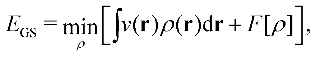 | (1) |
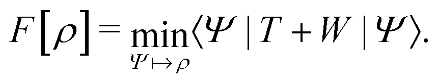 | (2) |
The term DFT expresses the fact that observables in the ground state at zero temperature can be considered as functionals of the ground-state density. This can then be extended to thermal equilibrium, etc., as others point out. So, it means that the density is a sufficient descriptor. It is important to say “can be considered as a functional of the density” and not “is a functional of the density”, because this is a choice: observables can also be considered as functionals of the many-body ground-state wave function, or the one-body Green's function, or many other possible choices. The functional of the many-body ground-state wave function is very simple (whereas the wave function is not, of course), and a density functional will in most cases be exceedingly complicated (whereas the density is simple). Actually, I chose to say “can be considered as”, because this does not imply that there must be an explicit expression.
A second important point: the density is not known a priori but is needed as input to evaluate our density functionals for a given system and observable. So, as a second aspect of DFT, we also have to invoke the variational character of the energy as functional of the density, because it allows us to find the density that is needed to evaluate the functionals for the various observables, without calculating the density from the many-body wave function. Otherwise, DFT could probably not compete with other approaches, not even as an idea – for example, also the external potential is a sufficient descriptor (for given particle number or chemical potential), it is simple, and it has the advantage that we (think we) know it. The variational character also has the benefit that a slightly wrong density may still lead to a reasonable energy (whereas this may not hold for other observables).
So, we may consider DFT as one possibility: one possible way to formulate the calculation of observables in a many-body system. There are many such ways, and we know that for most systems we will never be able to obtain the exact answer. Therefore, once we agree that those various ways are in principle exact, the true question is: how suitable are they as starting points for approximations? And so, for our purpose here: in which way is DFT a good starting point for approximations?
The theorem of Hohenberg and Kohn5 and the works by Levy6,7 and Lieb8 are beautiful mathematical treatments. Importantly, the basic concept that the ground-state electron density determines everything often enables decisive physical insight. The often misleading assumption is that the above laid out, exact algorithm “ρ(r)  ground-state energy (and even everything)” can be expressed in terms of a closed mathematical expression. Approximating the algorithm by a mathematical functional, i.e., by a DFA, suffers from the severe problem that the range of validity of this functional is typically unclear: We can test its accuracy only by comparing results with experiments or high-level wave-function theories. We trust the reliability for systems that we believe (!) are “similar” to the tested ones, but we don’t know about the accuracy for untested systems. And the term “similar” is not even defined.
Let me add: I am not aware of a proof that the exact exchange–correlation-functional exists, beyond the noted algorithm which requires to solve the many-body Schrödinger equation. However, and most importantly, the works by Hohenberg and Kohn and Kohn and Sham have shown the way to develop density-functional approximations which revolutionized the description and understanding of polyatomic systems.
Thus, approximate and exact density-functionals are mathematically quite different. The noncomputability of the exact functional indicates that systematically improvable DFAs are probably possible, in the sense of mathematical a priori error estimation – that is, mathematical statements towards an approximation's accuracy in terms of its adjustable parameters, such as basis size. Therefore, I would like to go out on a limb and say that approximate density functionals are not really approximations to exact density functionals. They are instead largely independent and, to a variable extent, semiempirical models that have the common use of the density as a basic variable as a characteristic. The latter aspect is for me an answer to the question “What is DFT?”
 | (3) |
For many years, the SIE had been assumed to be the main systematic error in DFAs, related to the incorrect dissociation of molecular ions, the underestimation of chemical reaction barriers and band gaps of molecules and bulk materials, the overestimation of polymer polarizability, and many other failure of commonly used DFAs.11,12 However, the development of two SIE-free functionals, the Becke0513 and the MCY214 functionals, changed the understanding.15 While these two exchange–correlation functionals, nonlocal and also nonsemilocal, are SIE-free by construction for any one-electron system and perform as well on thermodynamics benchmarks as hybrid functionals, they still retain significant errors in the dissociation of molecular ions, band gaps of molecules, and polymer polarizability problems, much like the hybrid functional B3LYP. The only significant improvement observed is in the prediction of reaction barriers. Thus the systematic error is clearly not the SIE.
To describe the systematic error of DFAs, the concept of the delocalization error has been developed, and it can be understood from the perspective of fractional charges.16,17 For systems of small or moderate physical sizes, conventional DFAs usually have good accuracy in total energies for an integer number of electrons. For a fractional number of electrons, conventional DFAs, however, violate the Perdew–Parr–Levy–Balduz (PPLB) linearity condition,18–20 which states that the exact ground-state energy E(N) is a linear function of the fractional electron numbers connecting adjacent integer points. Inconsistent with the requirement of the PPLB linearity condition, E(N) curves from conventional DFAs are usually convex, with drastic underestimation to the ground-state energies of fractional systems. The convex deviation of conventional DFAs decreases when the systems become larger and vanishes at the bulk limit. However, the delocalization error is exhibited in another way, in which the error manifests itself in too low relative ground-state energies of ionized systems and incorrect linear E(N) curves with wrong slopes at the bulk limit.16,17,21
To reduce or eliminate the delocalization error, enormous efforts have been devoted to the development of new exchange–correlation functionals. None of these developments are based on a semilocal form. All have nonlocal features in the functionals – see the development of the scaling approaches.22–25
In addition to the delocalization error characterized by fractional charges, commonly used DFAs also have a significant systematic static correlation error characterized by the violation of the constancy conditions on fractional spins.17,20,26 The combination of the exact fractional charge condition18 and the exact fractional spin condition20,26 leads to the general flat-plane condition,27 the satisfaction of which is a necessary condition for describing the band gap of strongly correlated Mott insulators. The flat-plane condition also leads to the conclusion that the exact exchange–correlation functional cannot be a continuous functional of the electron density or the density matrix of the noninteracting reference system everywhere.27 To reduce or eliminate the static correlation error, one has to use nonlocal functionals.28
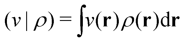
 as a function of the external potential v ∈ L3/2(
![[Doublestruck R]](https://www.rsc.org/images/entities/char_e175.gif) 3) + L∞(3) follows the existence of a universal density functional
3) + L∞(3) follows the existence of a universal density functional 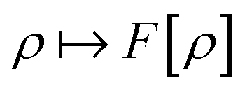 as a function of the electron density ρ ∈ L3(3) ∩ L1(3) such that5,8
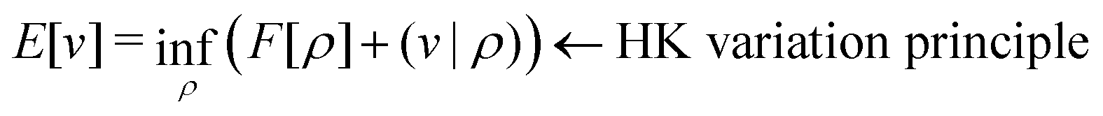 | (4) |
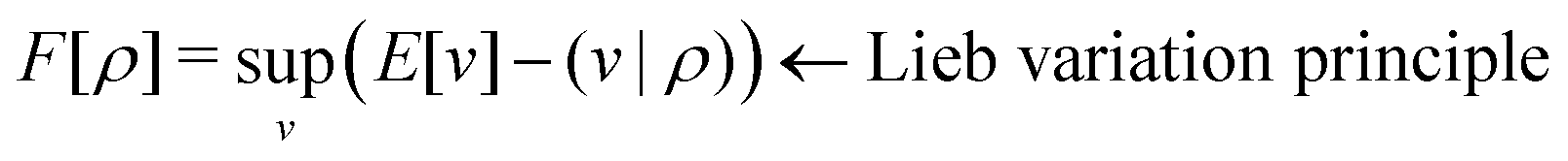 | (5) |
 . Since E and F can be calculated from each other, they contain the same information, only expressed in different ways. However, although the Lieb variation principle is a powerful tool for analysis and method development, it is not a practical tool for computation. Instead, the power of DFT derives from Kohn–Sham theory, making it possible to approximate F[ρ] (sufficiently) accurately and inexpensively for densities ρ of interest to us by introducing orbitals.
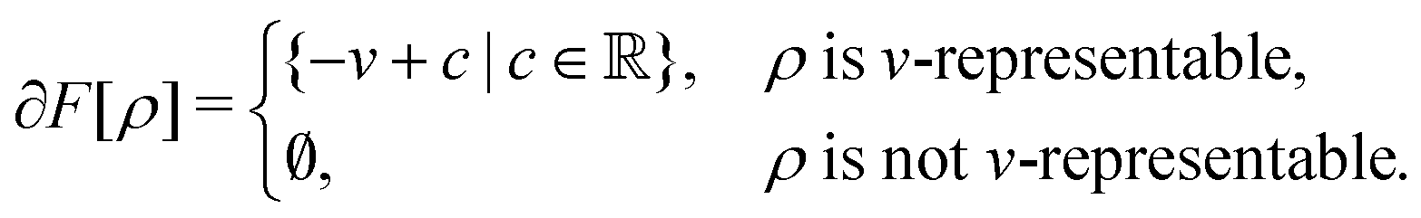
The Hohenberg–Kohn theorem,5 often thought of as the cornerstone of DFT, is easy to prove (apart from some subtleties) but perhaps not so easy to understand intuitively. Hohenberg and Kohn's original formulation of DFT is therefore not only restrictive in scope (in that it assumes v-representability) but may also appear a little mysterious.
Levy's constrained-search formulation6 took the mystery out of DFT and brought clarity and generality to the field – a major step forward, indeed. Lieb's convex formulation,8 on the other hand, gave DFT beauty and elegance by identifying the density functional with the Legendre transform (convex conjugate) of the ground-state energy, thereby placing DFT in a broader mathematical framework.32
It is an important and nontrivial result in DFT that the ensemble constrained-search functional and the Legendre-transform functional are the same – they are merely complementary formulations of the same thing.8 Together, they constitute the solid foundation of DFT.
Furthermore, comparing the situation with paramagnetic-current DFT, where the lack of a (corresponding) Hohenberg–Kohn theorem has been established by Capelle and Vignale,36 it is striking that although (ρ,jp) determines the nondegenerate ground state, if degeneracies are allowed, then the level of degeneracy is not determined.37 A given (ρ,jp) can therefore be associated with two different Hamiltonians (in fact, infinitely many) that may have different numbers of degenerate ground states. (Of course, this doesn’t stop the constrained search, which remains well defined.) In DFT, the extra layer of a Hohenberg–Kohn theorem (not just the first part of a constrained search) rules out such situations. I view the Hohenberg–Kohn theorem as a gold reserve – it is perhaps unexciting and just sits in the vault but is, on the other hand, good to have in certain extreme situations.
| E[v] = F[ρ] + (v|ρ) ⇔ −v ∈ ∂F[ρ] ⇔ ρ ∈ ∂E[v]. | (6) |
 | (7) |
The optimality conditions in eqn (6) give some additional insight: the ground-state energy E and the universal density functional F are functions whose subdifferential mappings (“functional derivatives”) are each other's inverses. Loosely speaking, therefore, E and F may be obtained from each other by differentiation followed by inversion and integration.
With such justification, one can approach the problem of finding this mapping in a completely different way – not by building approximations to the known exact solution (as done in the wave-function theory), but by parameterizing an empirical representation of the mapping device, the functional. Most DFAs are built upon mathematical representations of the functional grounded in our physical understanding of what it should look like (based on exact results for model systems), but one can envision finding the mapping without any such help from physics – for example, by brute-force training of a neural network (machine learning).38 One can, therefore, think of DFT as an empirical method that can be made exact.
While the blind brute-force (e.g., via ML) discovery of the density-energy mapping is, in principle, possible, it has important limitations compared to physically motivated DFAs. First, without any constraints due to physics, such brute-force search is going to be computationally wasteful. Second, having discovered the mapping between energy and density, one still has no recipe for computing energy derivatives with respect to various perturbations (i.e., properties), unless properties (or various energy derivatives) were included in the training. In contrast, using a physically motivated form of the functional opens access to properties (although the quality is not guaranteed, as illustrated by the developments of magnetic DFAs39).
To me, only orbital-free DFT is unequivocally DFT; everything else can also be fruitfully viewed from an alternative perspective. Indeed, some theoretical approaches and computational methods can legitimately be considered wave-function theories/methods, density-matrix theories/methods, propagator theories/methods, and density-functional theories/methods. I do not wish to take a hard line and proclaim that these types of theories/methods are not DFT because the philosophy (especially the emphasis on explicitly defining and characterizing the functional that is being approximated), traditions (especially the openness to pragmatic parameterization and approximation), and tools of DFT can be useful even for theories/methods that are “not just DFT”. But other, non-DFT, approaches could sometimes be even more useful.
But this is just one strategy. It is possible to determine additionally other contributions to the energy from the orbitals – for example, parts of the exchange energy in hybrid methods – or even to calculate all contributions to the energy exactly from the occupied orbitals, except the correlation energy. The latter can then be approximated by orbital-dependent functionals.40 In the latter case, the density is not needed at all in the calculation of the total DFT energy. If, furthermore, the orbitals are obtained via the optimized-effective-potential (OEP) method40–46 or within an appropriate generalized Kohn–Sham approach, then DFT methods results that do not require at any point the calculation of the density. The density is then only required in the underlying formalism.
I feel that the perception of DFT has been somewhat blurred by a questionable statement that, one way or another, is frequently found in textbooks and articles. This is the statement that DFT is distinguished from wave-function methods by using the electron density instead of a wave function to calculate the total energy of an electronic system. This statement is at least misleading if not wrong because most DFT methods used in practice are Kohn–Sham or generalized Kohn–Sham methods, which require orbitals and thus one-electron wave functions to calculate crucial parts of the total energy.
The common theme of these DFTs is the reduction of the inherent complexity of the direct description of a many-body system to the comparative simplicity of functionals of the density – either explicitly, or implicitly in terms of auxiliary functions such as orbitals. The strategy, in the time-independent case at least, is to obtain the relevant physics (hence also chemistry) by an appropriate minimization procedure on a functional of the density itself (whether it be pure-state or ensemble).
 γ
γ ρ, while the second map ρ
 Ψ
Ψ Γ employs the Hohenberg–Kohn theorem. It is its simplicity and compactness in the BBGKY sense and also its definite connection with a real world via its exactness that make DFT such a fertile ground for the present wealth of DFAs.
This great success of DFT can be favourably compared with a rather tumultuous development of “higher-order” full 1RDM or density-matrix-functional (DMFT) and 2RDM theories, which still do not enjoy a truly successful “take-off”. The ongoing development (see contribution (4.1.1)) explores a way64 in which DFT can help DMFT with such a “take-off”, while DMFT can help DFAs with the problematic inclusion in the latter of nondynamical or strong electron correlation.
2.2 What is Kohn–Sham DFT?
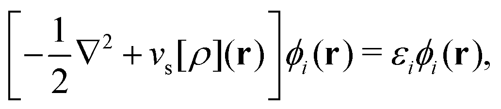
As a result, one can replace a many-body interacting Hamiltonian, H, by a simpler-to-evaluate one-body Kohn–Sham effective Hamiltonian:
 | (8) |
 , while the energy is given by E0[ρ] = Ts[ρ] + EHxc[ρ] + (v|ρ). We will define vs and EHxc below.
Formally, one may define 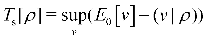 , where
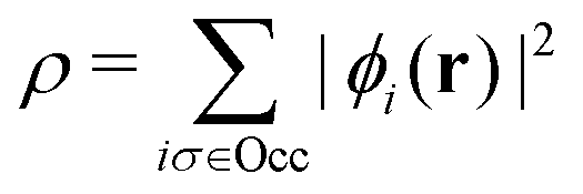
 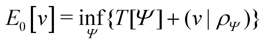 in the notation defined in contribution (2.1.13).‡ Thus, Ts[ρ] is the lowest kinetic energy of a noninteracting system with density ρ. Kohn–Sham DFT is useful because the Hartree–exchange–correlation (Hxc) energy,
| EHxc[ρ] := F[ρ] − Ts[ρ], | (9) |
vxc = ![[v with combining macron]](https://www.rsc.org/images/entities/i_char_0076_0304.gif) holexc + resp holexc + resp | (10) |
holexc and the response potential resp. This partitioning emerges from differentiation with respect to ρ of the exchange–correlation energy Exc[ρ] represented via the exchange–correlation pair-correlation function ḡxc,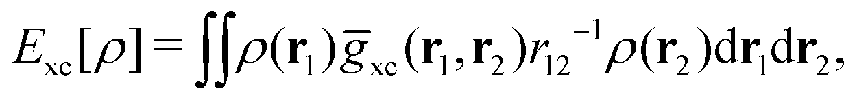 | (11) |
holexc, the derivative of the ρ functions under the integral, represents the universal interaction (for both occupied and virtual Kohn–Sham orbitals) with the exchange–correlation hole of the unit charge. In turn, the potential resp, the derivative of the pair-correlation function ḡxc, exhibits the spatial step-like structure, with the individual steps distinguishing various atomic and molecular electron shells.69
Ultimately, virtually all explanations of chemical behaviour are cast in orbital language, even if the underlying computations are based on the most sophisticated techniques of theoretical chemistry. The ready acceptance of DFT in chemistry has been greatly aided by the availability of the familiar orbital model. As for the old adage that Kohn–Sham orbitals and orbital energies “have no meaning, there is no Koopmans’ theorem like in Hartree–Fock theory”: the opposite is true.70,71
The orbital energies of almost all DFAs do not have the nice properties of the exact Kohn–Sham model, being some 5 eV too high (not negative enough). This is unfortunate and has some adverse consequences, but fortunately the upshift is approximately the same for the upper valence and the lower virtual (valence) orbitals, so the correct relative order is preserved in most DFAs. Nevertheless, more efforts should be made to construct DFAs that obey these exact Kohn–Sham properties (much) more closely.
This endows the theory with the ability to provide physically relevant quantities – for example, Dyson orbitals enter the expressions for photoionization/photodetachment cross-sections and can even be reconstructed from experimental data.74 Moreover, the orbitals provide a link between many-body theories and DFT – for example, one can judge the quality of a particular DFA by how well the shapes and energies of the Kohn–Sham orbitals agree with those from high-level many-body calculations (e.g., equation-of-motion coupled-cluster theory).78 These ideas are already exploited in optimally-tuned range-separated DFAs.76,77 But, perhaps more opportunities exist for using ab initio Dyson orbitals to build better DFAs?
Specifically, the electronic states of small metal clusters are bunched in shells. These shells are experimentally observed in the variations of polarizabilities, ionization energies, and electron affinities – to name a few characteristic observables. Kohn–Sham orbitals, as approximations to Dyson orbitals, reflect these shell structures in a large variety of free and ligand-stabilized clusters. Thus, the now common concept of superatoms in chemistry is based almost exclusively on Kohn–Sham calculations and the corresponding canonical Kohn–Sham orbitals.
Due to this, the Kohn–Sham orbital energies εi differ, in general, from the ionization energies Ii by the spectroscopic average of the satellite ionizations (see contribution (2.4.9)) as well as by the contributions from the response potential (see contribution (2.2.3)), with equality only for the highest occupied Kohn–Sham molecular orbital.71 The “well-behaved” (i.e., orthonormal) Kohn–Sham orbitals are, in no way, the “poor cousins” of the Dyson orbitals, forming a distinctively different set of “optimal” orbitals. Indeed, unlike the Dyson orbitals, the occupied Kohn–Sham orbitals meaningfully accommodate the “electron pairs” of conceptual chemistry, while their energies provide a fair estimate of the potentials of primary ionizations. Furthermore, combined with the virtual Kohn–Sham orbitals and their energies, they form the basis for the successful treatment of electronic excitations in TDDFT (see contribution (2.4.9)).
What is more logical than continuing along this line and taking out another part (the kinetic energy of some noninteracting system)? And what is more logical than taking this noninteracting system to be “similar” to the real system – with the same density, in the spirit of DFT? Generalized Kohn–Sham theory is then also very natural, both because we know more pieces and because (like the kinetic energy) we do not know them as explicit density functionals. Making these pieces and the resulting “potentials” more and more complex appears to build a continuous bridge between Kohn–Sham and Green's functions equations. Another generalization is to start with the consideration that the calculation of any observable will in general integrate out certain details of a system, so the same value for the observable might well be found in a simpler system. This holds for the density – with the Kohn–Sham system, for example – but one can also build auxiliary systems for other observables and profit from the Kohn–Sham experience.
Second, further to the discussion about the Kohn–Sham system, we should keep in mind that, for a single electron, the Kohn–Sham excitation energies equal the exact ones, while the Kohn–Sham electron addition energies are different from the exact ones. So we may expect that, for certain systems, there is a reasonable correspondence for the excitation energies. It is far from obvious that this would also hold true in extended systems with many electrons, and, of course, the Kohn–Sham gap does not equal the optical gap in general. The Kohn–Sham band structure is nevertheless a powerful starting point for calculations using, for example, one- and two-body Green's functions.
Third, the sometimes bad reputation of the Kohn–Sham noninteracting system stems from the fact that it is often used in place of the real system – not to yield simply its density, but also any other observable, in particular, spectral functions. Of course, this can lead to strong disagreement with the truth – and the band gap is just one example. Maybe we should just be more precise in saying what we are doing here – namely, that we use the Kohn–Sham expression (which is a functional of the density) for a given observable as an approximate functional because we do not know a better one? This doesn’t change the results, but it sounds a little more fair to the Kohn–Sham noninteracting system.
In molecules, it is well known that the Kohn–Sham HOMO–LUMO gap is much below the I–A difference. This is due to the fundamental difference that the Kohn–Sham system has an attractive potential due to the exchange–correlation hole of −1 electron also for the virtual levels, while the Hartree–Fock system lacks this attractive hole potential for the virtual levels. In the same way, the presence of this vholexc potential lowers the LUMO level (bottom of the conduction band, BCB) in solids strongly.81 The exchange–correlation hole in solids is pretty localized – at a given point r, its size is usually well within a unit-cell range around r and therefore its potential is strongly stabilizing. In a delocalized excitation, from an occupied Bloch state to an empty Bloch state, the excited electron does not benefit from this stabilization. Neither does an added electron – the excitation energy to this delocalized state is understandably close to the fundamental gap. So, physically we cannot expect the Kohn–Sham band gap to match approximately the fundamental gap or a delocalized excitation energy. Excitons in a solid (except for Frenkel excitons) typically have a large size, extending over many unit cells. They have excitation energies not much lower than the delocalized excitations, so also for them the attractive Kohn–Sham potential vholexc does not fit reality.81
The situation is different in molecules since there the physical hole that the excited electron leaves behind is roughly mimicked by the attractive exchange–correlation hole in the Kohn–Sham potential. Hence the Kohn–Sham virtual–occupied orbital energy differences have the nice property that they do approximate excitation energies in molecules;72,73 see contribution (2.4.9).
The difference between the Kohn–Sham band gap and the fundamental gap can be cast in the form of expectation values of the response potential part vresp of the Kohn–Sham potential;82 see also contribution (3.8.6).
The resolution of the apparent paradox is that the Kohn–Sham energy is not calculated as the expectation value of the Hamiltonian in the Kohn–Sham wave function. The moment we adopt the Kohn–Sham approach, the original Hamiltonian of the system is no longer relevant. We are dealing with a reference system that is no longer interacting, but the rules for calculating the energy from the orbitals have also changed and are now expressed in terms of the exchange–correlation energy functional of the density. One could argue that the “particles” of this reference system are the “quasiparticles” of the original system, and this may help to rationalize the a priori surprising success of the Kohn–Sham orbitals in predicting single-particle excitation energies.
A tongue in cheek observation would be that the Hartree–Fock model manages to build a determinant that has a little bit lower expectation value of the Hamiltonian, but it has to distort the orbitals (make them more diffuse) because the lowering of the kinetic energy then just outweighs the energy penalty of the increase in the electron–nuclear energy. The Hartree–Fock model does not care – it just tries to get the lowest energy determinant. As noted in contribution (2.2.12), the true power of Kohn–Sham DFT has to come from accurate approximations of the exchange–correlation energy (defined in the Kohn–Sham context), but the good properties of the Kohn–Sham orbitals are an asset of this model.
Although, undeniably the Hartree–Fock Slater determinant has the lowest energy among all Slater determinants, we now know that the Kohn–Sham determinant can at least match, if not beat that (record), since it is “energy optimal” in a similar sense: in the Hartree–Fock optimization, we use the full interacting N-electron Hamiltonian, H and then seek the lowest energy Slater determinant as the best approximate ground state. For the Kohn–Sham orbitals, we may perform an equivalent, but reverse Rayleigh–Ritz optimization: let us assume that the ground state Ψ of the physical N-electron, interacting system is somehow known (and fixed). Then, we consider all N-electron effective, noninteracting Hamiltonians, Hv, with a local potential v(r). The ground-state wave function and energy of each Hv are Φv and Ev, respectively.
For N > 1, Ψ cannot be the exact ground state of any of these noninteracting Hamiltonians, Ψ ≠ Φv for each v, because Ψ is an interacting state while all Φv are noninteracting states (Slater determinants). Hence, the following Rayleigh–Ritz energy difference on the left-hand side is strictly positive:
| 〈Ψ|Hv|Ψ〉 − Ev > 0. | (12) |
I note that the variational principle in eqn (12) can be used to construct optimally converging power series expansions for the Kohn–Sham potential, without using the adiabatic connection (AC) path formalism.85
The orbital energies for the frontier HOMO and LUMO were rigorously shown to be the DFA prediction of the negative of the first IP and the first electron affinity (EA) in 2008.21 Three key results were used in the proof. (1) The Janak theorem shows that Kohn–Sham orbital energies are the derivatives of the total energy with respect to the orbital occupation numbers. Note that the Janak theorem does not relate orbital energies to any physical observables.87 (2) The left and right derivatives of the total energy with respect to the total electron number, or the left and right chemical potentials, are the negative of the first IP and the first EA, respectively, of the corresponding energy functional. This follows from the linear condition on the behaviour of the total energy for fractional number of electrons.18 The linearity condition is true for the exact functional, or for a functional without delocalization error for general systems. For infinite bulk systems, however, the linearity condition holds true for any functional approximation.16 (3) The chemical potentials were proved to be the derivatives of the energy with respect to the orbital occupation numbers of HOMO and LUMO in a Kohn–Sham calculation, when the exchange–correlation energy used is a functional of the density. With the use of the Janak theorem, this then establishes that the Kohn–Sham HOMO and LUMO energies are the chemical potentials of the system for the given DFA.21 Similarly, when the exchange–correlation energy is a functional of the noninteracting one-electron density matrix, the chemical potentials were proved to be the derivatives of the energy with respect to the orbital occupation numbers of HOMO and LUMO in a generalized Kohn–Sham calculation.21 Therefore, the HOMO and LUMO orbital energies are the DFA prediction of the negative of the first IP and the first EA. This interpretation of the HOMO and LUMO energies holds true for molecular and bulk systems, for any given DFA.
Indeed, DFAs with minimal delocalization error23–25 have excellent predictions of IPs and EAs from the HOMO and LUMO of generalized Kohn–Sham calculations, comparable to the accuracy of GW approaches.88 In addition, the orbital energies above the LUMO and below the HOMO approximate the corresponding quasi-particle energies, with similar accuracy as the HOMO/LUMO for the IP/EA. This has been explored to describe accurately the excitation energies and conical intersections of molecular systems in the quasi-energy DFT approach based on ground-state generalized Kohn–Sham calculations.88,89
The attractive properties of the exact Kohn–Sham orbitals and orbital energies have been expounded in some contributions; see contributions (2.4.9), (2.2.4), (2.2.13), and (2.2.11). A salient feature of the exact Kohn–Sham model is that the LUMO is not at −A (given that the HOMO is at −I) but much lower: the HOMO–LUMO gap is approximately equal to the first excitation energy.72,73,90 It should be made clear that contribution (2.2.15) does not contradict these properties of the exact Kohn–Sham model. It refers to a different family of Kohn–Sham models, usually called the generalized Kohn–Sham models. These generalized models make it possible to include, for instance, part of the exchange operator (a nonlocal potential) of the Hartree–Fock model and adjust the local part of the potential so that the density remains exact and adjust the exchange–correlation functional so that the energy also remains exact.67 In such a scheme, the orbital energies are different from those generated by the exact local Kohn–Sham potential. In such a generalized Kohn–Sham model, one may strive to obtain that the HOMO is again at −I and that the LUMO is now at −A, as is also done in the Koopmans-compliant functionals.91,92 The LUMO then becomes more diffuse and one loses the simple representation of excitations in TDDFT with just one or a few orbital transitions.73
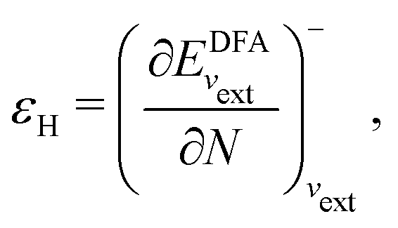
In an inverse approach, the local potential is determined up to an arbitrary constant. Thus, in principle, the absolute values of the orbital energies are not defined. However, if the correct asymptotic condition on the potential is satisfied, which also sets the constant, then εH = −I is obtained, where I is the experimental ionization energy, if an exact density is given (row 1 Table 1). Similarly, a good approximation to the experimental −I is expected if a good approximation to the density is given from a DFA calculation (row 1 in Table 1). However, the corresponding LUMO energy has not been shown to relate to the ionization energy and is not a good approximation to the experimental −I, as discussed in contribution (2.2.16). In atomic calculations, the unoccupied-orbital energies, {εa}, obtained from inverse Kohn–Sham calculations, have been shown to represent electronic excitations, with εa − εH describing excitation energies of the system with the same number of electrons. Using εa − εH to approximate excitation energies for molecules is less successful.
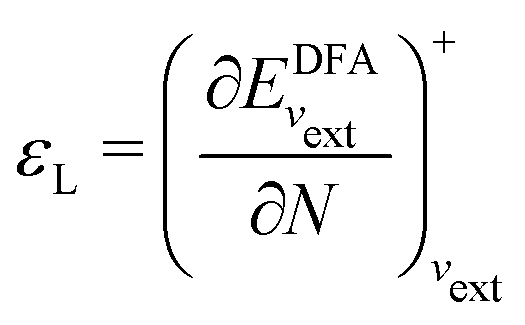
 ; see Chen et al.,95 Voora et al.;96 (2) agreement of the HOMO orbital energy εH with
 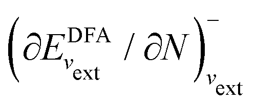 the chemical potential of electron removal for the functional employed; (3) agreement of the LUMO orbital energy εL with
 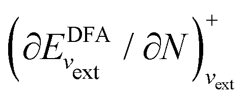 the chemical potential of electron addition for the functional employed. No entry indicates that it is impossible or not yet known how to conduct the corresponding calculation. (Table provided by Yang, extended from ref. 93)
| Noninteracting system | Type | E DFT | E DFAxc[ρσs(r)] | E DFAxc[ρσs(r′,r)] | E DFAxc[{ϕpσ}, vext(r)] | |
|---|---|---|---|---|---|---|
a In an inverse calculation, the potential is determined up to an arbitrary constant and the absolute values of the orbital energies are therefore undefined. However, if the correct asymptotic condition on the potential is imposed, which also sets the constant, then εH = −I, is obtained, where I is the experimental ionization energy.86
b If the correct asymptotic condition on the potential is imposed, and if a good electron density is obtained from the DFA, then the inverse OEP calculation will leads to εH that is a good approximation to the experimental −I.
c The agreement between ρσs(r) with  is only true at the complete basis set limit for the basis set expansion of vσs(r), and not so for any finite basis set.93
d Similar to (b), if the correct asymptotic condition on the potential is imposed, then the direct OEP calculation will lead to εH that is a good approximation to the experimental −I.
e For explicit functionals of the density, or the density matrix, GOEP/OO gives the same total energies and density matrix as in regular SCF. But the orbitals obtained in general are no longer the canonical orbitals and thus have no orbital energies directly. However, a unitary rotation can bring them to the canonical orbitals with proper orbital energies in agreement with the corresponding chemical potentials.
f In GOEP or OO calculations, the Hamiltonian for the noninteracting system is not available, so neither are the noninteracting orbital energies. is only true at the complete basis set limit for the basis set expansion of vσs(r), and not so for any finite basis set.93
d Similar to (b), if the correct asymptotic condition on the potential is imposed, then the direct OEP calculation will lead to εH that is a good approximation to the experimental −I.
e For explicit functionals of the density, or the density matrix, GOEP/OO gives the same total energies and density matrix as in regular SCF. But the orbitals obtained in general are no longer the canonical orbitals and thus have no orbital energies directly. However, a unitary rotation can bring them to the canonical orbitals with proper orbital energies in agreement with the corresponding chemical potentials.
f In GOEP or OO calculations, the Hamiltonian for the noninteracting system is not available, so neither are the noninteracting orbital energies.
|
||||||
| Inverse KS/inverse OEP vσs(r) | Inverse | ρ σ s(r) | Yes | Yes | Yes | Yes |
| ε H | ||||||
| ε L | No | No | No | No | ||
| KS vσs(r) | Direct | ρ σ s(r) | Yes | |||
| ε H | Yes | |||||
| ε L | Yes | |||||
| OEP vσs(r) | Direct | ρ σ s(r) | Yes | Yes/noc | No | |
| ε H | Yes | |||||
| ε L | Yes | No | ||||
| GKS vσs(r,r′) | Direct | ρ σ s(r) | Yes | Yes | ||
| ε H | Yes | Yes | ||||
| ε L | Yes | Yes | ||||
| GOEP/OO vσs(r,r′) | Direct | ρ σ s(r) | Yes | Yes | No | |
| ε H | Yese | Yese | ||||
| ε L | Yese | Yese | ||||
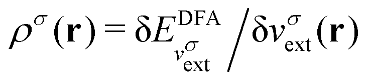
In a direct calculation with a DFA – that is, when the energy is minimized with respect to its variables, as discussed in contribution (2.2.15) – the HOMO energy of the noninteracting reference system has been shown to be equal to the chemical potential for electron removal
 | (13) |
 | (14) |
There are other approaches to direct calculation, using as the basic computational variable either a local potential vσs(r) in an OEP approach or a nonlocal potential vσs(r,r′) in the direct generalized OEP (GOEP) approach.94 The meaning of HOMO and LUMO energies in direct OEP calculations was established in ref. 21; see also Row 3 in Table 1.
In Table 1, we also list the results on the agreement of the electron density of the noninteracting reference system with the density of the physical system as defined by the linear response.93
Particularizing to the ground state, Kohn–Sham DFT is, at base, the decomposition of the Levy–Lieb functional (putting aside to a separate discussion the issues associated with the original Hohenberg–Kohn and later Levy–Lieb functionals) into physically recognizable, interpretable, and computable parts. Orbital-free DFT (better called one-orbital DFT) exploits only the decomposition, while conventional Kohn–Sham DFT also uses the Kohn–Sham orbitals explicitly. Both variants (to use a currently prominent word) are fundamentally Kohn–Sham theory. Both have the same definitions of kinetic energy, Hartree energy, exchange energy, and correlation energy. All those definitions depend upon the Kohn–Sham determinant.
The distinction between those two variants is operational – namely, what is done to exploit the Kohn–Sham decomposition computationally. This is crucial because of the many statements that one sees to the effect that orbital-free DFT is an “alternative formulation of DFT” that avoids the problems of Kohn–Sham theory, etc. That completely ignores the underlying Kohn–Sham logic. That logic is in fact crucial to constraints on approximate kinetic-energy density functionals (KEDFs).
Then, instead of complaining about “the idiosyncratic behaviour” of the Kohn–Sham exchange–correlation potential, one should fruitfully explore and employ this meaningful information – see, for example, contributions (3.1.12) and (3.8.6). Moreover, one should not attempt to “wash away” this precious true information by constructing artificially too smooth Kohn–Sham exchange–correlation potentials by “reverse engineering” techniques.
As to the generalized Kohn–Sham scheme, the term ‘Kohn–Sham’ seems to be misused in this case. Indeed, out of desire to get electron affinities as the energies of virtual orbitals, the original Kohn–Sham theory is forcefully “crashed” in some (out of infinitely many) variants of the generalized Kohn–Sham “landscape” by mixing different theories both globally and with range-separation techniques.
Traditionally, the Kohn–Sham orbitals are used only to evaluate the kinetic energy of the Kohn–Sham model system, which represents the bulk of the full kinetic energy, taking into account the fermionic nature of electrons. The Kohn–Sham orbitals, however, contain much more information than their kinetic energy. The occupied Kohn–Sham orbitals, for example, enable an exact calculation of the exchange energy. This means that all parts of the total energy except the correlation energy can be easily calculated exactly, technically by evaluating the Hartree–Fock energy with Kohn–Sham orbitals. Indeed, approximating only the remaining small part of the energy, the correlation energy, is a natural and systematic approach. For individually approximating the correlation energy, orbital-dependent functionals40 can be constructed that use occupied as well as unoccupied Kohn–Sham orbitals and their orbital energies, in this way exploiting much more of the information contained in the Kohn–Sham model system.
Historically, this route was not pursued for three reasons:
(1) to avoid the high cost of evaluating the exact exchange energy, which nowadays is not really a problem for molecules up to a size of several hundred atoms. For larger systems or when very many electronic-structure calculations are required, in ab initio dynamics simulations, for example, the cost of exact exchange remains an issue.
(2) to benefit from error cancellation between exchange and correlation contributions. While this is a valid reason, the cancellation is not complete, limiting the accuracy that can be reached by traditional Kohn–Sham methods.
(3) to avoid the problem that the exchange potential is not directly accessible in terms of the Kohn–Sham orbitals. With the OEP method, functional derivatives of orbital-dependent energy expressions, including – for example, the Kohn–Sham exchange potential – are accessible.40–46
While basis-set OEP methods were numerically problematic in the past, robust, numerically stable basis-set OEP methods are now available.46 Moreover, orbital-dependent functionals can be evaluated in a post-self-consistent-field (post-SCF) manner, avoiding the need to take functional derivatives of orbital-dependent functionals with respect to the electron density. Alternatively, functional derivatives can be taken with respect to orbitals instead of the electron density, leading to generalized Kohn–Sham methods.
Meta-GGA and hybrid functionals are established functionals that depend on the occupied orbitals. Correlation functionals based on the adiabatic connection fluctuation-dissipation (ACFD) theorem100,101 depend on unoccupied as well as occupied orbitals and their eigenvalues. The simplest example of such a functional is the correlation energy within the random-phase approximation (RPA).102–104 All these methods are Kohn–Sham methods or, depending on the way the exchange–correlation potential is obtained, generalized Kohn–Sham methods.
This is a crucial distinction between gas-phase chemistry and materials physics and chemistry. For those with access to significant computing resources, exact exchange is not prohibitive for the comparatively small number of calculations needed to study an isolated molecule of up to a few hundred atoms. But that is manifestly not true for ab initio molecular dynamics (AIMD) of several thousand molecular-dynamics (MD) steps used to screen tens of different but kindred condensed-phase systems, for each of which the constituents are molecules with 300 or more non-hydrogen atoms. This distinction illustrates the compelling importance of continued effort to improve lower-rung DFAs. It also is but one example that there is more than gas-phase chemistry at stake in the development of DFT methodology and algorithms.
Despite the lack of a rigorous theory that would allow one to construct them in a systematic way, a potentially useful pragmatic solution within the Dirac–Coulomb–Breit framework has been known for a long time. Since relativistic effects become important at high densities – that is, in exchange-dominated core regions – one could, in a first approximation, restrict oneself to an appropriate treatment of the exchange energy. For the exchange energy of the relativistic homogeneous electron gas (RHEG),57,59,109 a multiplicative correction (a kind of “enhancement factor”) has been derived as a simple analytic function Φ(β), where β = (3π2ρ)1/3/c (in atomic units). This function satisfies Φ(β) > 1 and tends to one at the low-density limit; it is a sum of both Coulomb (longitudinal) and Breit (transverse) contributions. This scheme has been implemented and tested for atoms at the LDA level110 and subsequently extended to the GGA level111via data on the linear response of the RHEG to a weak perturbing potential.57 Data for several small diatomics are available as well.112
While valence-shell related properties turned out not to be sensitive with respect to these corrections,112 a high sensitivity of core one-electron energies of heavy atoms has been clearly demonstrated.111 For heavy atoms, these corrections seem to be of the same order of magnitude as atomic (nonrelativistic) correlation energies.110 So far, it appears that these corrections have not yet been implemented into a molecular or solid-state code. Obviously, studies of the impact on core-related properties will be of interest. Recently, short-range LDA and GGA exchange functionals have been developed and implemented in a similar way,113,114 but again only for atoms and ions so far.
A very recent development of a potentially useful relativistic local hybrid functional115 within an X2C code should be mentioned as well.
2.3 What can be described with DFT?
In practice, we do Kohn–Sham DFT, which in addition to the density and the ground-state energy (in principle, both exact) also gives us the Kohn–Sham noninteracting wave function, from which many more properties of the system can be obtained, but only approximately, given that the Kohn–Sham wave function is a noninteracting approximation to the exact many-body wave function.
We are of course free to use the Kohn–Sham wave function as a zero-order starting point for a many-body treatment – but we are then leaving the domain of DFT.
Again, this is actually not completely the case. Take the polarizability – we do go beyond the Kohn–Sham independent particle polarizability, by adding Hartree (i.e., the bare Coulomb interaction in the integral kernel of the Dyson equation) effects in the RPA, and even exchange–correlation effects through the exchange–correlation kernel, which is also a density functional. Like Görling in contribution (2.3.2), you might object that this is TDDFT, but I would say it is linear response in the ground state, so we are talking about functionals of the ground-state density. Simply, we have derived this ground-state density functional using TDDFT, but who cares how we derived it once we have it? We could of course dream of finding simpler functionals for the polarizability, maybe even explicit functionals of the ground-state density, but since even the kinetic energy is so difficult, I wouldn’t bet on this in the near future.
For an N-electron system, a Kohn–Sham calculation with an exchange–correlation functional that is an explicit and continuous functional of the electron density leads directly to Ev(N − 1) and Ev(N + 1), the ground-state energies of the corresponding (N − 1) and (N + 1) electron systems. Similar connections follow for a generalized Kohn–Sham calculation with an exchange–correlation functional that is an explicit and continuous functional of the noninteracting reference density matrix. This is true because of the following: (1) it has been proved that the HOMO/LUMO energy is the chemical potential for electron removal/addition,21 (see Table 1) (2) the PPLB condition shows that the chemical potential of the N-electron system is −I and −A.18 Thus the band gap can be predicted from the HOMO–LUMO gap, in either Kohn–Sham calculations with an explicit functional of the electron density or generalized Kohn–Sham calculations with an explicit functional of the noninteracting reference density matrix. This connection is independent of the functional approximation. However, the accuracy of the prediction depends on the quality of the functional used.21 For functionals with minimal delocalization error, the prediction is comparable to, or better than, that of GW approaches.25,88,89
Similarly to the access to the ground state information of the corresponding (N − 1) and (N + 1) electron systems, it has been argued recently that ε(N), the orbital energies of orbitals above LUMO and below HOMO also approximate the corresponding quasiparticle energies ω+/−(N) as follows: εm(N) ≈ ωm+(N) = Em(N + 1) − E0(N), and εn(N) ≈ ωn−(N) = E0(N) − En(N − 1). This then links directly to the excited-state energies of the corresponding (N + 1) and (N − 1) systems.88,89,116,117 Extensive numerical evidence supports this claim.88,89,116,117 Thus, the excited-state energies of N electron systems can be obtained from ground-state calculations on the (N − 1) or (N + 1) electron systems.88,89,116,117
2.4 What concepts are useful for the development and understanding of DFT?
This has important practical consequences. In particular, local and semilocal approximations predict incorrect energies and densities for a diatomic molecule AB in the dissociation limit. In fact, these approximations are much more accurate for integer than for fractional electron numbers. This problem still plagues density functional approximations. A non-self-consistent cure is to evaluate the approximate functionals on Hartree–Fock densities, which localize an integer charge around each separated nucleus.118 Doing that also cures some related problems, such as spurious charge transfers at smaller internuclear separations.
The first widely recognized hybrid DFA is Becke's half-and-half functional.124 It was derived based on a linear model for the AC path, which was then empirically extended, leading eventually to the widely used B3LYP functional.126–129 More sophisticated AC models have been used to develop and rationalize the popular “nonempirical” PBE0 functional,130 as well as some other hybrid functionals.131
The AC formalism has provided an important playground for the development of the advanced DFAs that involve the unoccupied Kohn–Sham orbitals. The random-phase approximation (RPA) was introduced to the DFT community via the ACFD formalism.100,132 Görling–Levy (GL) perturbation theory133 shows that the initial slope of the AC path is twice the second-order GL perturbation energy (GL2). For systems with a linear AC path, the exact exchange–correlation functional is therefore nothing but the exact exchange plus GL2 correlation energy.134 The AC formalism has motivated the initial developments of several successful double-hybrid approximations by further mixing the second-order perturbation (PT2) energy with the already successful hybrid functionals.134–137
Another way to use the SCE limit in chemistry is to build interpolation models of the AC between the Kohn–Sham limit (which may include exact exchange and second-order perturbation theory) and the expansion at strong coupling strength.142,148–151 The interpolation strategy based on global quantities (integrated over all space, a strategy that can be viewed as creating nonlinear hybrids and double hybrids) was abandoned for some time because of its lack of size consistency. However, more recently, it has been shown that size consistency can be easily restored for these functionals at no extra computational cost.150
Such calculations can also be used to extract the coupling-constant-dependent one- and two-particle density matrices. The one-particle density matrices may be used to define an AC focusing on the kinetic component of the DFT correlation energy – see, for example, ref. 125 and 158, as alluded to in contribution (2.4.8) and calculated in ref. 159. The two-particle density matrices can be used to give direct access to the exchange–correlation hole and its coupling-constant average.149,160 All these quantities can be determined using high-level ab initio methods, giving valuable insight into the near exact behaviour of F[ρ]. The challenge is to parameterize simple models to construct useful DFAs – work that is still an active area of research.
All of the AC pathways mentioned above focus on the density-fixed case, relevant to Kohn–Sham DFT. However, if one notes the conjugate relationship between F[ρ] and E[v], a natural alternative is a potential-fixed AC, a possibility that has also been explored numerically.154,161 Since the density is no longer fixed, the calculations of the AC pathway are in the potential-fixed case much simpler to perform, but the noninteracting reference system (the bare nucleus system) is farther from a realistic electronic system than its Kohn–Sham counterpart. Recently, other ACs have been developed that do not insist on a fixed density along the AC pathway – see, for example, ref. 162 for an AC that recovers the Møller–Plesset series as its low coupling-strength expansion. The utility of the AC as a concept for understanding new theories based on these alternative pathways and their relative pros and cons compared with the Kohn–Sham approach underlines its importance as a concept in electronic-structure method development.
Increasingly, however, interpolations along local ACs have been used, meaning that the coupling-strength (λ) integration is applied to the corresponding energy density or even to the exchange–correlation hole followed by integration over one and two spatial coordinates, respectively. While the existence of a “local AC” has never been proven rigorously, Becke argued that such an approach does not violate any basic principles and is just a matter of changing the order of integration that is valid for continuous functions165 – see also, for example, ref. 149.
One of the first applications of the local AC to the development of DFAs was to derive the B88 correlation functional166 Given that the global AC is the founding principle underpinning (global) hybrid functionals (see contributions (2.4.2), (2.4.4) and (2.4.6) above),124,128,167 a local AC should be relevant for local hybrid functionals (LHs) with position-dependent exact-exchange admixture. Let us mention in passing our early attempts to derive local mixing functions for LHs from local AC interpolation.168 Other important hyper-GGA functionals simulate strong correlation effects and also make use of local interpolations.165,169
Most notable in this context are recent efforts to include the SCE limit (λ → ∞) of the AC by local AC interpolation.149,170–172 Importantly, the local AC approach has advantages compared to the global AC in terms of achieving size-consistency for DFAs in the presence of degeneracies.173
Generalized Kohn–Sham theory, recently extended to both TDDFT174 and ensemble DFT,175 provides a useful viewpoint that rigorously justifies the use of nonmultiplicative potentials. In particular, this means that the use of Fock-exchange potential operators (and variants thereof) in hybrid functionals (both global and range-separated), originally viewed as an ad hoc and theoretically unjustified merger of Kohn–Sham and Hartree–Fock theories, are rigorously derived and justified within generalized Kohn–Sham theory.176 While, for a given system, there is only one exact Kohn–Sham map, there are infinitely many partially-interacting systems to which an exact generalized Kohn–Sham map may be formed.68 This added flexibility has been found to be useful for spectroscopy – in particular, for choosing generalized-Kohn–Sham maps in which the derivative discontinuity is eliminated; see elaboration in contribution (4.1.5).
In ab initio quantum chemistry, the route that is followed, in many different ways, consists of finding computationally feasible and sufficiently accurate approximations to the full configuration-interaction (FCI) solution. One may call this a mathematically-oriented approach. One can view DFT as an attempt – maybe often unconsciously – to follow the route of finding physical models for the pair-correlation function. The largest part of the LDA functional is the exchange functional, which is practically the same as Slater's original ρ4/3 approximation. Slater derived his “exchange hole” from a simple model (local hole of constant depth integrating to −1) which leads to practically the same exchange energy expression (with ρ4/3 density dependence) as the homogeneous electron gas of LDA. But the Slater construction shows that the interpretation is not necessarily that of an electron-gas exchange approximation. Indeed, it has been realized that this simple local hole is much more like an exchange–correlation hole – for instance, accounting for considerable left–right correlation in the chemical bond (which is why it soon was called an exchange–correlation approximation).69 The Slater (or LDA) hole yields much better bond energies for prototypical diatomic molecules than the exchange hole of the Hartree–Fock model: bonding changes from severe underbinding in Hartree–Fock theory to some overbinding in LDA. Also, the systematic errors in frequencies and bond distances that characterize the Hartree–Fock model disappear. This tells us that modelling of the exchange–correlation energy may not be so difficult after all.
The major improvement in the step from LDA to GGA comes from improved modelling of the exchange approximation. Becke's parameterization was fitted to reproduce the exchange energies of the rare-gas atoms, and Perdew's nonempirical GGA approximation of the exchange hole likewise considerably improved atomic exchange energies. The main contribution to the success of GGA (improvement over LDA) for bonds in simple diatomic molecules originates from these exchange improvements. This is mystifying since one would expect the better exchange approximation of GGA to reproduce more closely the poor Hartree–Fock results. Apparently, the GGA exchange improvements have turned the exchange holes into better exchange–correlation holes. So, there is still a considerable lack of precise understanding why the most successful models work, which perhaps explains the lack of consistent improvement beyond the GGA level. On the other hand, the “physical route” to the correlation problem by modelling of the exchange–correlation hole is hopefully a fruitful way forward that can be pursued independently of the clarification of the mathematical intricacies of DFT.
(i) the exchange energy functional (and the exchange hole) changes linearly under uniform coordinate scaling. The correlation energy (and hole), by contrast, does not exhibit any simple scaling. However, when the electron–electron interaction becomes dominant with respect to the kinetic energy (see contributions (2.4.5) and (4.5.8)), then the exchange–correlation energy scales again as the exchange energy.170,177,178 It might thus make sense to have an exchange-like functional to capture (at least part of the) static (left–right) correlation.
(ii) More recent work by Burke, Perdew and coworkers (see ref. 179 for a recent review) has clarified the sense in which LDA is a universal limit for coulombically bound systems, with exchange as the leading term.
For example, NTOs afford a unified and rigorous description of electronic transitions in terms of MO theory, which is also experimentally verifiable, noting that observables such as absorption cross-sections can be rigorously expressed in terms of matrix elements between hole and particle NTOs. By using natural orbitals and their occupations, one can compare such properties as diradical character and the number of effectively unpaired electrons;180 although not observable, these quantities are useful for understanding the underlying electronic structure and for judging whether DFT captures the physics of the problem.
The same observation, coupled with the fact that the quality of the response of the density depends on the quality of the density, also enabled the extension of Kohn–Sham DFT to electronic structures that have multiconfigurational character and, therefore, are not well described by the single determinant. Although with exact Kohn–Sham DFT, we should be able to treat any type of electronic structure, current DFAs implicitly rely on the expectation that a single Slater determinant provides a good zero-order representation of the wave function; consequently, most Kohn–Sham DFAs fail when the electronic structure is multiconfigurational.
In the spin-flip DFT (SF-TDDFT) approach, the “difficult” multiconfigurational states (such as diradicals, molecules with broken bonds, transition metals) are described by means of spin-flipping excitations from a well-behaved high-spin reference state.181–183 In exact DFT, this approach should yield identical results to the traditional Kohn–Sham treatment – however, with the current incarnations of Kohn–Sham DFT, the SF-TDDFT method provides an effective solution to certain types of multiconfigurational states.
Thinking in terms of response properties also helps to understand when to anticipate potential problems. For example, while a TDDFT calculation may yield excellent excitation energies for a few valence states of interest, it may fail miserably in describing nonlinear properties, such as two-photon cross-sections, if the chosen functional does not treat (higher-lying) Rydberg states correctly.
2.5 What useful concepts of electronic structure theory have emerged from DFT?
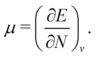 | (15) |
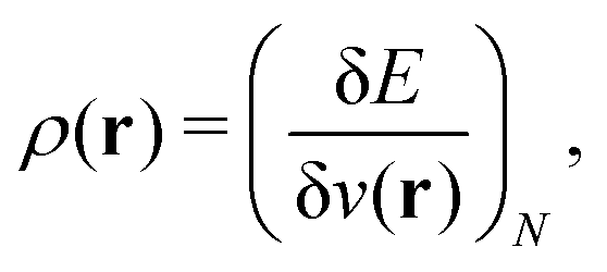 | (16) |
This observation forms the basis of conceptual DFT where, starting from the energy functional E[N,v] for atoms, molecules, and the solid state, derivatives of the type  are identified as response functions of the system's energy to perturbations in N and v, important for chemical reactions, with μ and ρ being the first-order (n = m + m′ = 1) responses. Second-order properties (n = 2) like the chemical hardness,
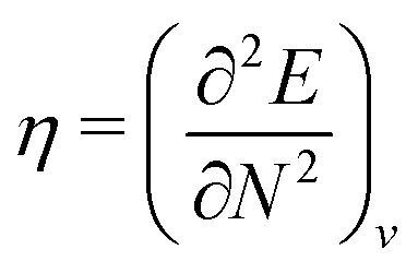 | (17) |
 | (18) |
 | (19) |
 | (20) |
All these response functions and some others derived from the energy function E(N), of which the electrophilicity ω is the most eminent representative,190,191 were shown to bear chemical relevance. To give some examples: the chemical hardness η in eqn (17) was identified with Pearson's hardness, while the Fukui function f (r) was recognized as a generalization of Fukui's frontier MO concept, its product with the total softness, the local softness s(r) = Sf(r) being a local indicator for soft regions in a molecule.
The first conceptual development of the chemical potential μ was based on the assumption that the fundamental functional E[N,v(r)] is differentiable everywhere for both variables.186 Subsequently, the exact piecewise linear conditions at fractional particle numbers were established originally by Perdew, Parr, Levy, and Baldus (PPLB)18 based on grand canonical ensembles at zero temperature and later by Yang, Zhang, and Ayers based on pure states with degeneracy.20
The piecewise linearity of E[N,v(r)] with respect to N means that the derivatives at integer electron numbers are discontinuous. In particular, at a given integer N, the chemical potential μ = (∂E/∂N)v, the Fukui function f (r) = (∂ρ(r)/∂N))v and other related quantities are discontinuous, the corresponding left and right derivatives being different. In view of this discontinuity, use of the derivative notation is best understood with an underlying finite-difference mathematical definition,47,192 where e.g. the right derivative is obtained by evaluating E(N + 1) − E(N). This interpretation is particularly important for second derivatives such as the chemical hardness in eqn (17).47 Since the chemical hardness describes the change in the first derivative at an integer electron number N, it will be zero or infinite at N and have no physical meaning unless interpreted in the above finite-difference manner. The PPLB condition is thus the foundation for the discussion of derivatives. It leads to the identification of the left and right chemical potentials with the ionization energy I and the electron affinity A, respectively.18 This identification was used to establish the physical meaning of the HOMO and LUMO orbital energies as the density-functional prediction of −I and −A, respectively, associated with the functional approximation used.21
Steric effects have been quantified in DFT by the Weizsäcker kinetic energy functional.195 Its functional derivative has been employed to predict stereoselectivity.196 Pauli energy has been validated as a robust identifier for double, triple, quadruple, and even higher covalent bonds.197
A difference between AC-DFT and multiconfigurational AC theory is that, in the former theory, the electron density is fixed to the exact density by a local one-body potential varying along the AC path, while in the latter, the condition of a constant density is imposed as an approximation. AC-based correlation energy approximations have been used with MCSCF, complete-active-space SCF (CASSCF), density-matrix-renormalization group (DMRG) and geminal theories.205,206 These multiconfigurational AC approximations rely on the ACFD formalism and the (extended) RPA. An appealing feature of the multiconfigurational AC methods is that only one- and two-electron reduced density matrices are needed, as opposed to perturbation approaches such as complete-active-space second-order perturbation theory (CASPT2) or N-electron valence-state second-order perturbation theory (NEVPT2), which require three- and four-body RDMs.
It has been recognized that, in the general AC theory, the reference state need not be an electronic ground state as long as it is not degenerate. This has motivated the development of AC methods for excited states, which recover the dynamical correlation energy for a specific state.207 It may be worth exploring if a similar approach could be developed for Kohn–Sham DFT, taking an excited Kohn–Sham determinant as the noninteracting system. The clear advantage over TDDFT would then be the description of states of double-excitation character.
The long-range electron correlation energy naturally emerges as the difference between the energies of the FCI wave function and the chosen model (CI, CASSCF, etc.).210,211 The short-range correlation energy is rigorously defined as
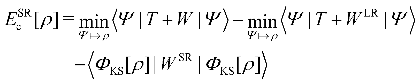 | (21) |
The rigorous range separation of electron correlation has led to a proliferation of wave-function methods using short-range exchange–correlation functionals as an inexpensive way of accounting for dynamical (short-range) correlation, thereby improving their accuracy and/or efficiency.212 A promising direction of development of DFT via its merger with wave-function theory is enabled by gaining access to a correlated two-particle local function – the on-top pair density – which can be used as a variable in correlation functionals in addition to the electron density; see, for example, ref. 213 and contribution (4.1.1).
This situation changed in the mid 1990s when the tight-binding (TB) semiempirical theory was proposed as an approximation to Kohn–Sham DFT,215,216 based on previous work of Foulkes and Haydock.217 The current theoretical view on TB methods, which in the meantime have been consistently parameterized for the whole periodic table,218 is based on a Taylor expansion of the total energy E around a reference density ρ0, constructed as a sum of atomic valence densities:
| E[ρ] = E(0)[ρ0] + E(1)[ρ0,δρ] + E(2)[ρ0,(δρ)2] + E(3)[ρ0,(δρ)3] + … | (22) |
The speed-up of a TB calculation compared to, for example, a regular GGA(PBE) DFT calculation, is about three orders of magnitude, at little loss of accuracy for common properties like electronic and geometric structures. Thermochemical data and, in particular, conformational energies are generally not so well described, which is at least partially attributed to the small (mostly minimal) AO basis sets employed.218 The development of more accurate, but still sufficiently fast, TB methods is an important future field that should take advantage of more advanced DFAs.
A further simplification of Kohn–Sham DFT implementations can be achieved by using the approximate density from the variational fitting of the Coulomb potential for the evaluation of the exchange–correlation energy and potential.228,229 The resulting energy expression remains variational and yields optimized structures and relative energies that are almost indistinguishable from standard Kohn–Sham approaches, but at a substantially reduced computational effort. The extension of this auxiliary DFT (ADFT) approach to perturbation theory permits first-principles molecular property calculations of systems with up to thousand atoms – for example, second-order analytic energy derivatives.230 Most recently, ADFT also serves as platform for the development of new DFAs.
Orbitals obtained from the solution of the Kohn–Sham equations are also at the basis of most many-body perturbation theories solving, in approximate manners, the Dyson and Bethe–Salpeter equations (GW and BSE methods). These approaches have brought tremendous progress in understanding properties of solids, in spite of some lack of accuracy, and almost all of them (for solids) are based on DFT.
3 Density functional approximations
3.1 What strategies have been useful in constructing DFAs?
The second category, promoted by the Minnesota team, has led to functionals involving up to 64 parameters. These functionals may be very accurate for – but limited to – small classes of molecular systems and properties. In a paper involving 200 combinations of exchange and correlation functionals,233 Mardirossian and Head-Gordon compared the performance of these exchange–correlation functionals applied to 82 data sets, with and without dispersion corrections, and documented the scattering of the performance among the properties for given classes of molecular systems.
Of course, these two approaches are often combined. The most accurate functionals (including meta-GGAs, hybrids, and RPA-like functionals) generalize Kohn–Sham theory67 by employing as arguments of the energy density not only the electron density and its gradient, but also the occupied or even the unoccupied orbitals or one-electron wave functions, and by optimizing those arguments. A sometimes important but seldom discussed step in the development of a functional is “deconstruction”: removing what is wrong or unnecessary, as in the transition from gradient expansions to generalized gradient expansions.123
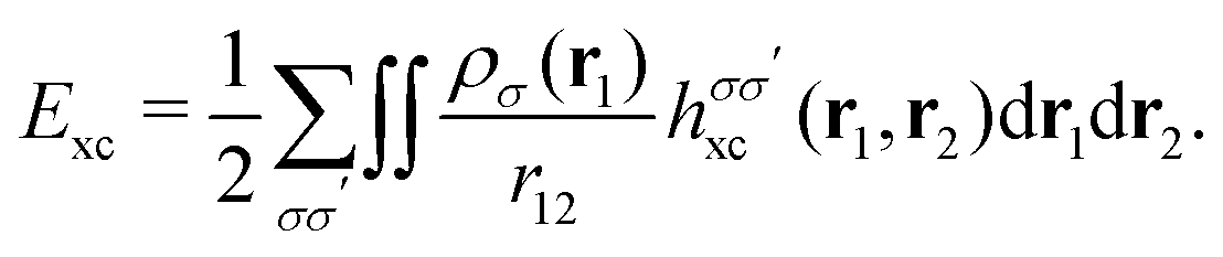 | (23) |
Another useful strategy in the development of GGAs is to enforce a large-gradient limit of the enhancement factor,248,249 which ensures an accurate treatment of nonbonded repulsion in van der Waals complexes.250,251 Such functionals are capable of high accuracy for modelling intermolecular interactions in both gas-phase and solid-state systems, when paired with a density-functional dispersion correction.252
Interestingly, since the introduction of Becke's half-and-half model, constraints derived from properties of the AC have been used for functional development, thereby avoiding introducing variables to be fitted to external (not theoretical) data. In other words, increasing the number of theoretical constraints in going from local to hybrid functionals leads to improved numerical performance (at least within the same functional family) for a large number of chemical properties.257
Also, the time-dependent version of the SSE262 has been very useful in the context of TDDFT. For example, one can show that the TDDFT exchange–correlation kernel fxc can be written exactly as two contributions, one responsible for the shift of the Kohn–Sham band gap to the fundamental gap and the other accounting for excitonic effects.263 This splitting has been recently used to calculate accurate optical spectra of semiconductors and insulators within a pure Kohn–Sham TDDFT framework – that is, without invoking empirical information nor theory beyond Kohn–Sham DFT (e.g., GW theory) to correct the Kohn–Sham gap.264
A useful strategy for deriving approximate functionals for interfaces may be based on an approximate treatment of the screened Coulomb interaction and of dielectric matrices; the latter may then be used to derive approximate hybrid functionals with parameters that capture how the dielectric screening varies in different parts of the system (see, e.g., ref. 265 and references therein).
3.2 How accurate do we need DFAs to be?
| Property | Accuracy required |
|---|---|
| a Savin: mean value of the experimental uncertainties compiled in ref. 266 for over 500 molecules containing elements with Z < 18. See also ref. 267. b Savin: Q95, cf. contribution (3.3.12), obtained from the experimental uncertainties compiled in ref. 266 for over 500 molecules containing elements with Z < 18. c Savin: heat of formation divided by (the number of atoms −1), justified by the mean of the values obtained by detaching successively one atom after the other. d Grimme: molecular total energy difference for the same covalently bound structure but with different three-dimensional shape normally obtained by rotation around covalent bonds. e Schwerdtfeger: based on ref. 267. f Kronik: an experimental accuracy of 0.1 eV in band gap measurements is possible, as well as desirable, but not at all trivial and may require the combination of several measurement techniques. Many reported experimental results, especially for insulators, do not necessarily reach this level of accuracy. Also, some reported band gaps arise from correction terms to optical gap values. Furthermore, experimental band gaps are also influenced by electron-nucleus coupling, sometimes quite significantly. This should be taken into account when comparing to results of electronic structure theory that do not include such coupling. g Helgaker: the uncertainties in experimental bond lengths depend strongly on the experimental technique used – an accuracy of 1 pm for covalent bonds of first-row atoms is a reasonable target for computation. For benchmark data of wave-function methods, see ref. 268. h Draxl: for vibrational frequencies, even semilocal DFT does already very well, if computed consistently (i.e., for the optimized geometry269). The situation is more tricky for intensities, as these are typically not measured for solids. The situation may be different for molecules; thus a distinction would be needed. Note that intensities can’t be obtained by DFT alone. i Kaupp: the necessary and achievable accuracy for shieldings and relative shifts differs from nucleus to nucleus and for different applications. The best way to report the accuracy that allows a comparison between different nuclei, is to give relative deviations in %, normalized to the shielding or shift range of a given nucleus (either computed or experimental). For meaningful accuracy, this should not exceed a few percent, sub-percent accuracy is better, and is achievable at least for light main-group systems. This is not yet the case for transition-metal nuclei. j Schwerdtfeger: these accuracies are expected from any decent ab initio calculation. For comparable accuracies for EFGs achieved by coupled-cluster methods see ref. 270, for DFT see ref. 271 and 272. | |
| Heats of formation | 1a kcal mol−1 |
| 3b kcal mol−1 | |
| Heats of formation (“intensive”)c | 0.3a kcal mol−1 |
| 1.6b kcal mol−1 | |
| Conformational energies | 0.1d kcal mol−1 |
| Barrier heights | 1e kcal mol−1 |
| Ionization potentials | 1e kcal mol−1 |
| Band gaps | 0.1f eV |
| Excitation energies | 0.1f eV |
| Bond lengths | 1g pm |
| Vibrational frequencies | <3h cm−1 |
| Shielding constants | 0.5–5%i |
| Dipole moments | 0.1–0.2j D |
| Dipole polarizabilities | 0.5–1j a.u. |
| Electric field gradients | 0.1–0.2j a.u. |
In extended systems, it is often impractical to repeat calculations with different functional approximations [see contribution (2.1.16)], and it is essential to develop a level of “trust” [see contribution (3.2.7)] in the approximations one uses and a feeling for their limitations. My own applications over several decades show a clear preference for main-group elements, which might imply less trust in the ability of particular DFAs to describe transition and rare-earth elements. This is perhaps not surprising, since some DFAs describe energy differences in the corresponding atoms very poorly.
Moreover, if we have an incorrect long-range behaviour of the one-particle density, then the region close to the nucleus will also suffer because of charge conservation. As a result, properties like electric-field gradients (EFGs) are not so well described by currently available DFAs – the worst results are perhaps obtained for the late transition metals.271 To illustrate, the Cu EFG in CuF at the experimental bond distance is measured to be (in atomic units) −0.31(2), while some representative DFAs give +0.495 (LDA), +0.444 (PW91), and +0.146 (B3LYP). At the coupled-cluster CCSD(T) level, we have −0.439 (−0.341 if relativistic effects are included).270 To address this problem, the parameters in the CAMB3LYP functional can be tailored such that accurate results for EFG (and other short-range properties) are produced,272 but this is not a nice solution and no unique functional exists that performs well for all properties concerned.
One should also mention that, as for molecules,273 the performance of various DFAs for the solid state has been extensively analysed in the past – see, for example, ref. 274–276. Here, a few percent error range is typical for solid-state properties such as lattice constants, cohesive energies and bulk moduli if (for the heavier elements) relativistic effects and (for the lighter elements) phonon contributions are included. For finite temperatures, thermal effects need to be included as well.
Another aspect to consider here is that the most important primary application of current Kohn–Sham DFT in chemistry is probably the determination of equilibrium structures (Re) including those of chemical transition states. Even with rather simple DFAs (e.g., GGAs), basically no severe outliers are obtained, even in electronically difficult cases – a fact that, in retrospect, was extremely important for the development of computational chemistry. As such, newly proposed, empirical DFAs, should be carefully tested not only for energies but additionally for the computation of Re structures. Similar considerations hold for the computation of vibrational frequencies, which are of utmost importance for thermostatistical properties – for example, Gibbs free energies.
Another aspect is that we may overemphasize the accuracy of what we take as a reference. Herbstein discusses several factors that may affect the measurement of such basic data as single-crystal unit-cell dimensions.282 Cioslowski et al. show that experimental error bars are often missing or can be quite large.266 Sometimes advanced wave-function calculations are not pushed far enough to be used as a reference.283
There have been a huge number of publications assessing the performance of different DFAs within TDDFT for the prediction of excitation energies both using theoretical and experimental reference data – see, for instance, ref. 284–288. Nonetheless, two difficulties are becoming nowadays evident: the reliability of affordable theoretical reference methods for large molecular systems may be difficult to assess, and the fact that excitation energies may not be the only property needed to provide a full answer to a given chemical question.
Concerning the first point, thanks to a number of detailed studies that compare DFAs results with those obtained using different reference methods, it has become evident that, especially for complex molecular systems, assessing the accuracy of DFAs is also dependent on the choice of reference. By targeting an accuracy below a certain threshold in the excitation energy, one is probably simply targeting the error bar of the methods used as reference.289 Furthermore, errors depend on the type of excitations considered – for instance, local or charge-transfer excitations. Due to the different impact of the approximation used in a given DFA on the different types of excitation, it is very difficult to assess a global accuracy for this DFA in predicting excitation energies. More severely, (vertical) excitation energies are often not what one aims for as a chemical answer since the quantitative description of the photophysical properties of a given molecular system are related to the prediction of its entire spectrum (absorption or emission), practically manifested in the observed colour.290 In this case, the accuracy we would like to reach – and which is asked for in industrial application, for instance – is the sensitivity of human colour perception.291
To achieve this objective, one needs to combine a very high (and energy-dependent) accuracy in the excitation energy with a very good description of the band shape. This latter is mostly obtained using approaches enabling the description of the vibrational broadening, that is the vibronic coupling between ground and excited states. Previous studies291 have nonetheless demonstrated that the same DFA can seldom reproduce with the same accuracy both electronic excitation energies and vibrational broadening. Finally, the comparison with experimental data can become even more complicated if environment effects, usually modelled with approximate methods, have to be considered.292 This latter point is of course of relevance, for any theoretical approach used and not exclusively limited to DFT.
From another point of view, comparison with experiment requires vibrational corrections to geometric parameters and zero-point energies. The situation for main-group elements is again very satisfactory, with latest-generation DFAs in conjunction with second-order vibrational perturbation theory (or anharmonic treatments) providing remarkably accurate results without the need for any scaling factor.294,296 The above remarks concern isolated molecules (or low-pressure gas-phase). The situation is more involved in condensed phases, where much work to improve the accuracy of the results is ongoing.
For example, it is commonly accepted that achieving a 1 kcal mol−1 (chemical) accuracy for binding energies involving covalently bound molecular species is often desirable, but setting a similar accuracy target for activation energies, which can be on the order of 1 kcal mol−1 in some processes and more than 10 kcal mol−1 in others, may be misleading. Furthermore, one can have reaction mechanisms that involve larger and smaller barriers along the same reaction pathway or along multiple competing pathways. A 1 kcal mol−1 accuracy level does not work well for noncovalent interactions either. In fact, even the frequently mentioned value of about 0.1 kcal mol−1 may not be adequate in this case.
If we replace the error criteria for the binding energies in weakly bound species and activation energies by relative errors of, say, 5%, then we may be in a better position to judge and make recommendations regarding what method to use. Indeed, if the activation energies along the reaction pathway of interest are on the order of 10 kcal mol−1 or more, as in ref. 298, then ∼5% relative errors translate into total errors on the order of 0.5–1 kcal mol−1, which is good enough to understand the reaction mechanism. However, if the activation barriers are on the order of 1–5 kcal mol−1, or if we must decide if a particular reaction has a barrier or is barrierless, as in ref. 299, then a fixed accuracy criterion may be insufficient to make a proper recommendation regarding what method to use. Similarly, a fixed 0.1 kcal mol−1 criterion might be of little use for some noncovalent interactions, where there are many cases in which the interaction energies are as small as 1 kcal mol−1 or less and equally many cases in which the interaction energies are on the order of a few kcal mol−1 or more. A good illustration of the former situation is the magnesium dimer, which is an important weakly bound system in studies of ultracold and collisional phenomena and which is characterized by a binding energy of about 430 cm−1; see ref. 300 and 301. To properly understand this system, one must be able to reach an accuracy on the order of a few cm−1, which is a major undertaking, even for the highest levels of ab initio wave-function theory.301,302
The magnesium-dimer example is also a reminder that in setting accuracy targets, we should be careful about treating wave-function methods, including those based on coupled-cluster theory, as providers of reliable reference information. As is very well known, wave-function methods exhibit a much slower convergence with the basis set than methods based on DFT. Also, the treatment of core electrons is usually different in DFT and wave-function calculations. Wave-function calculations are often carried out with frozen core electrons, whereas DFT (putting aside the issue of relativistic effective core potentials) is an all-electron theory. Thus, judging DFAs by comparison with wave-function approaches may sometimes be misleading or questionable.303 Finally, the CCSD(T) approach, often regarded as a standard for high-accuracy calculations, fails not only in multireference situations, such as covalent bond stretching and biradicals, but also in many cases of noncovalent interactions, including the aforementioned magnesium dimer, where the CCSD(T) binding energy extrapolated to the complete basis-set limit has a substantial error.301,302 While the development of ab initio wave function methods can be well served by comparisons with FCI, the development of DFAs may be better served by comparisons with reliable experimental data.
The idea of setting up accuracy targets using relative (percent) errors may easily be extended to other properties in Table 2. For example, the aforementioned 5% error limit would work well for vibrational frequencies, including low-frequency and high-frequency modes. Clearly, depending on the nature of the application, one may replace the 5% target by a different target.
Add to that something little discussed in this roundtable – namely, that predictive screening of materials requires even-handed accuracy across states of aggregation. One must have the same computationally affordable functional and protocols for both the isolated molecular constituents and the condensed phases, with correspondingly consistently appropriate accuracy for both constituents and aggregates. It is of little or no use in first-principles computational materials physics to prescribe a highly sophisticated DFA of great accuracy for the molecular constituents that cannot be afforded in condensed-phase studies or is deliberately tuned (e.g., OPTX) to be accurate for molecules only.
holexc + resp, where the overbar indicates that we are dealing with coupling constant integrated quantities; see Section 2.4. The exchange–correlation hole potential is directly related to the exchange–correlation energy density, holexc(r) = 2εxc(r) with 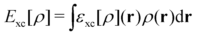 . The response part originates from the functional derivative of the εxc factor in the total energy.
Given DFAs with good total energies, the error in the orbital energies should not come from the hole part of the exchange–correlation potential – indeed, it has been argued that the error is in the response potential.320 It is quite common that an approximation to an integrand is decent in the sense that the integral (the energy) is well approximated, while the derivative of the integrand (the potential) is still very poor.
The response part of the current DFA potentials is too repulsive over the bulk molecular region, causing the 4–6 eV upshift of the orbital levels. A better approximation to the response potential is called for, rather than just the derivative that arises from existing LDA or (meta-)GGA energy density approximations. Indeed, replacing the LDA/GGA response part of the potential with the approximate response potential from ref. 321 (a local potential determined from nonlocal input) already improves the orbital energy spectrum a lot.320 Better approximations to the Kohn–Sham potential of course also improve response properties such as (hyper)polarizabilities and excitation energies.258 Note that this improvement is not primarily an effect of the correct asymptotic behaviour since the orbital energies are mostly determined by the potential in regions where the orbitals have a large amplitude (i.e., the region where the bulk molecular density resides). Obviously, the accuracy of the DFA potential has been lagging far behind that of the energy. It needs to be improved, preferably in a more fundamental way than by pragmatically admixing some percentage of a nonlocal exchange potential.
The OEP method has a bad reputation because of numerical problems. However, these problems have been solved and computationally efficient, numerically stable OEP methods are now available.46 An exact treatment of exchange requires correlation functionals that go along with it. Such correlation functionals exist – for example, RPA-based functionals102–104 – but are so far not very popular. The poor orbital energies are thus the price to pay for approximating exchange and correlation together in most DFAs, in order to exploit error cancellations.
I am aware of brilliant attempts to develop correlation functionals on top of self-interaction free references (discussed in the preceding contribution by Görling). I would be delighted to see this approach receive even more attention in functional development.
This should give us pause for thought when we want to blame the SIE for failures of DFAs. How much SIE is there really in the current DFAs? The DFA error in the orbital energy is of a different order of magnitude: 6.88 eV above the exact H-atom value with LDA and 6.20 eV when the B88 gradient correction is added – clearly, not the same effect as the tiny SIE in the total energy. The effect on the orbital energies that we call SIE arises when we take the functional derivative of the energy (it is in vresp).
A general definition of SIE is not so easy to formulate. In the original Perdew–Zunger work, the total energy was taken as starting point for constructing the correction.10 The most important effect of the Perdew–Zunger correction was, however, to change the potential and most of their discussion was focused on orbital energies. A straightforward definition of the SIE (also in the many-electron case) would be the error incurred by the exchange–correlation hole not integrating to −1 electron. Now, the first exact property that is required of the model holes in DFT is that they do integrate to −1 electron, as is already true for Slater's ρ1/3 approximation. This does indeed lead to reasonable results for the total energy but does not guarantee a good potential because of deficiencies that appear in the step to the corresponding potential.320
Using exact exchange (100% or at least a very large percentage) in either a generalized Kohn–Sham or EXX-OEP manner also provides a large improvement in the orbital energies, as noted in contribution (3.2.14). The improvement is due to the way the step to the potential works out in that case, as it does for the Hartree–Fock-like correction in the Perdew–Zunger self-interaction correction.
Görling was the first to point out that we can use Poisson's equation to define an effective charge density from the Kohn–Sham potential.43 Then, the Laplacian of the Kohn–Sham Hartree-exchange–correlation (Hxc) potential vHxc(r) defines unambiguously an effective charge density ρrep(r) whose Coulomb potential is the Hxc potential:
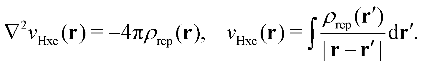 | (24) |
We agree with Baerends that the quality of the total energy in local and semilocal DFAs is (far) superior to the quality of the Kohn–Sham potential and hence we have decided not to interfere with the total energy of the DFA. Instead, we impose constraints on the effective local potential to reduce the self-interaction errors from it. These constraints, Qrep = N − 1 and ρrep(r) ≥ 0, are enforced with the OEP method, whose mathematical (rather than numerical) problems with finite basis sets are now well understood.323,324
The computational cost of these OEP calculations is determined by the matrix elements of the DFA functional derivative, a local potential, and is comparable to performing a small number (about ten) of DFA calculations. Imposing these constraints, the error of the HOMO Kohn–Sham orbital energies for local and semilocal DFAs reduces to about 1 eV. For one-electron systems, the two constraints give correctly a zero Hxc potential.325,326
From the perspective of fractional charges,16 an integration approach has been developed for the double-hybrid functionals,331 whose justification lies in the fact that they are found to fulfil better the piecewise linearity condition (see contribution (2.4.1)) and suffer less from delocalization error.332 Furthermore, the extended Koopmans' theorem333 (EKT) can be applied to the double-hybrid (DH) functionals, leading to the EKT-DH methods,334 which are shown to be capable of describing the breakdowns of the quasi-particle approximations for the inner-valence IPs, at a relatively low computational cost and a high accuracy.
3.3 How should we validate the quality of DFAs?
This procedure, sometimes requested by reviewers, is often time consuming. In addition, if one asks authors to benchmark each DFA for every type of compound in every type of reaction, it can be argued that one is perhaps approaching a new level of parameterization.
The development of standardized test sets has been very beneficial for the development of DFT. It would seem beneficial, yet challenging, to include a wide range of additional data in the development of new functionals to come closer to co-convergence.
This is why statistics such as the MAE should not be used to estimate the confidence level of a DFA. There are more pertinent metrics such as Q95 (the 95th quantile of the absolute error distribution), on which a level of confidence can be based.343,345 We then know that there is a 5% risk to get an absolute error above Q95. By comparison, the probability for absolute errors to be above the MAE has been observed to vary between 0.2 and 0.45.346 From a MAE value of let us say 0.5 kcal mol−1, one cannot estimate the probability/risk for the errors to exceed 1 kcal mol−1.
The confidence we have in the prediction capabilities of a given method has something to do with probabilistic forecasting; this however, may depend on factors difficult to quantify, such as deciding about the probability we consider good enough to take a decision. Ideally, a DFA should be judged on its prediction uncertainty, like any measurement method, but this requires the correction of systematic errors, which goes beyond the realm of the DFA itself.347–349
Let us now ask ourselves what is smallest target accuracy that is reached by 95% of the systems in this data set. It turns out that, to satisfy this condition, the target accuracy must be as large as 3–5 kcal mol−1, the presence of the interval arising from the finite size of the data set. Nevertheless, the B3LYP functional is a very successful DFA.
Related to this problem of adjusting the “useful” accuracy to the problem at hand is the question of what else is needed for a successful chemical prediction or interpretation? For example, we have learned the hard way that getting accurate electronic energies from coupled-cluster theory will not necessarily lead to more accurate chemical predictions. In real-life chemical applications, there are other important error sources, for example coming from solvation or entropy effects. In addition one can not stress enough how important it is to carefully construct the computational model. In studying complex molecules (or enzyme active sites), one needs to pay a great deal of attention to possible alternative conformers, alternative protonation states, possible hydrogen bonds or potentially functionally important solvent molecules, to name only a few important aspects of model construction. In our experience, the errors stemming from failing to treat any of the mentioned effects correctly can easily overwhelm the error in the electronic energies. If this is the case, focusing on computing accurate electronic energies on irrelevant chemical models or with a large, possibly unrecognized solvation energy error in the background appears rather pointless – the conclusions drawn from the calculations will likely be wrong or will fail to properly explain the experimental findings. These aspects require a great deal of chemical common sense on the part of the computational chemist and are independent of the intrinsic accuracy of the chosen theoretical method.
Sometimes statements on the validity of DFAs made in the literature are inaccurate or just not correct because a detailed analysis of numerical approximations has not been carried out before assessing the accuracy of the DFA. It is important to realize that the impact of poorly converged numerical calculations on the assessment of the validity of the theory is not the same for all properties and hence numerical verification should be done for each property of interest separately. It is also important to keep in mind that many comparisons of various DFAs in the solid state are made using pseudopotentials that are not consistent with the level of theory adopted for the valence electrons. For example, almost all hybrid DFT calculations are carried out with PBE pseudopotentials; and all comparisons are thus tainted by this inconsistency.
3.4 Where do existing DFAs work and where do they fail?
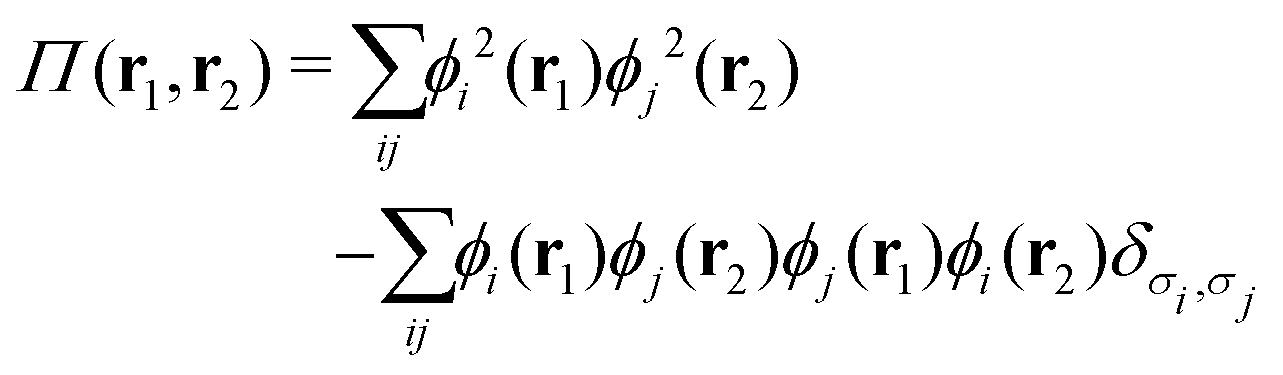 | (25) |
Notably, the form of the pair density gives rise to the exchange hole in the case of parallel spins (δσi,σj = 1) and leads to a depletion of probability of finding a second, same-spin electron near a reference electron. However, for multideterminental wave functions, the pair density behaves quite differently. Instead of leading to a Fermi (exchange) hole, with a depletion of parallel-spin electron density around a reference point, multireference systems can instead have a Fermi “heap” around the reference point,351 with an accumulation of parallel-spin electron density. This physics is not captured by Kohn–Sham DFAs, which model a localized exchange hole.
While there are other types of systems (such as those exhibiting significant delocalization error) where a particular DFA or class of DFAs may fail, all Kohn–Sham DFAs fail for multireference systems. Examples include stretched covalent bonds,352 organic biradicals,353 and solid Au2S.354
This is not an esoteric formal remark. In open-shell transition-metal complexes, for example, the multiplet problem is extremely prevalent and affects all of their physical (spectroscopic) properties in a profound way. Take a simple L-edge (2p → 3d) excitation. In a d5 system, this excitation leads to as many as 1512 different final states that all contribute to the L-edge absorption spectrum. Yet, in a particle–hole theory such as TDDFT, one only has 15 particle–hole pairs to work with. How to describe 1512 states with only 15 particle–hole pairs is not clear. In practice, the failures are dramatic. Another example are the d–d spectra of these ions, which frequently show low-lying double excitations that are completely absent from the DFT-computed spectra.355
Similar remarks hold for many multideterminental (as opposed to multiconfigurational) problems, like spin-coupled open-shell ions. Surely, broken-symmetry DFT is a highly useful tool, yet it is a bit of a crutch and I am not aware of a satisfactory formal solution that would also be practical.
I find it important to distinguish between multideterminental and multiconfiguration problems. In the former case, there is a single electronic configuration but spin coupling of the unpaired electrons leads to a multideterminental wave function. In the latter case, there is an actual mixing of configurations with different orbital occupations. The former case is far easier and far more frequent. Recognizing this distinction may help (and, in fact, has already helped) to design more tailored approximations – for example, spin-flip methods.
Focusing on my own experiences, the widely used B3LYP functional is among the best DFAs for studies of the activation barriers that determine aerobic oxidations of alcohols by gold nanoparticles,298 the BP86 and B97-D functionals performing considerably worse. At the same time, B3LYP and other hybrid functionals work poorly and the BP86 (especially when corrected for dispersion) and B97-D functionals are impressively accurate in applications of DFT to methyl–cobalt bond dissociation and low-lying excited states of methylcobalamin.357,358
The latter situation is similar to that created by the application of various DFAs to dicopper–dioxygen structural motifs. For example, when examining isomerization curves connecting the bis(μ-oxo) and μ-η2:η2-peroxo isomers of Cu2O2 cores supported by 0, 2, 4, and 6 ammonia ligands, hybrid functionals fail, the magnitude of the error being directly proportional to the percentage Hartree–Fock exchange in the functional.359 Pure GGAs work well in this case.
There is nothing new in the observation that pure GGAs may work better in situations involving static correlation. However, improving predictability of the outcome of DFT computations, so that one could, for example, avoid calibrating DFT functionals every time a new system is studied, while addressing fundamental issues such as the issue of SIE, would be useful. I realize that there has been great progress in addressing these and related issues in all sorts of interesting ways, but an additional effort toward improving the situation in this area would be helpful for the users of DFT methods.
Pantzasis362 pointed out that Kohn–Sham DFT generally fails to reproduce the experimental spin ladder for such systems (unless some ad hoc spin purification is performed), and thus the calculation of the magnetic coupling constant, and a more physical representation of the low-spin states requires a multireference treatment based on restricted-active-space SCF (RASSCF) or DMRG wave functions. However, also within the context of a large active space, a post wave-function treatment is needed. Multireference pair-density functional theory (MC-PDFT) starting from a large active space (DMRG or RASSCF active space with 30 electrons in 22 orbitals) gives encouraging results.363
Another important direction towards including strong-correlation effects also makes use of the AC but extends it to the strongly-correlated (λ → ∞) limit.149,170,172 While the question of how to best represent the noninteracting reference system of Kohn–Sham theory and the validity of the AC for multireference cases is still open, these approaches provide some hope of obtaining functionals that incorporate such effects.
The paramagnetic phase of transition-metal oxides – which is systematically described as metallic, contrary to experiment – is a paradigmatic example. These systems are a challenge also for more advanced methods such as the GW method.365 However, this problem arises since we are modelling the paramagnetic phase as nonmagnetic. Trimarchi et al.366 have recently shown that band-structure theories can give a correct description of these systems provided that one models the spin-disordered paramagnetic phase using a larger supercell.
In fact, this is routinely done to model the spin-ordered antiferromagnetic phase: the nonmagnetic unit cell is doubled so that a different spin can be specified for the transition-metal atom. In this case, a band-gap opening is usually obtained in band-structure theories, reflecting the fact that, the more physical information is put into the problem, the less accurate a theory needs to be.
Maybe I can clarify this point with the simple example of the Hubbard dimer at one-half filling, which can give insight into a paramagnetic or an antiferromagnetic spin structure, depending on whether or not the spin symmetry is broken. In the atomic limit (where the electron–electron interaction dominates over the kinetic energy, hence we are in the regime of strong correlation) the two electrons, one with spin up and the other with spin down, are localized one on one site and the other on the other site with equal probability – that is, the ground state is the spin singlet 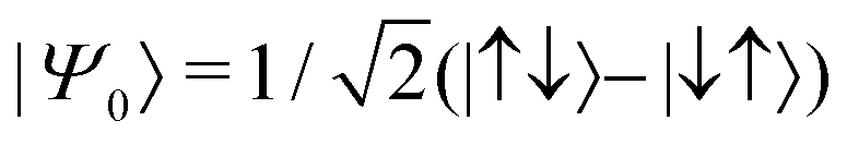 . The spectral function (which is related to photoemission spectra) thus shows, for each spin, two peaks with the same spectral weight 1/2 – one for the removal of an electron (peak at ε0, which is the orbital energy), and one for the addition of a second electron (peak at ε0 + U, with U the on-site electron–electron interaction), representing, respectively, the removal and addition energies, of an isolated atom with one electron.
Even the GW method cannot reproduce this spectrum. The GW method gives only one peak at ε0 + U/2, in line with the fact that this method describes many paramagnetic insulators as metallic. This happens because the GW method treats the charge/spin density as a classical charge distribution, with half an electron with spin up and half an electron with spin down on each atom that respond to the additional electron or hole added to the system in a photoemission experiment. If one considers instead the spin-symmetry broken state |Ψ0〉 = |↑↓〉 (or, equivalently, |↓↑〉), which is also an eigenstate of the system in this limit, then the GW method gives the correct spectral function. In this case, the electrons have fixed positions and one does not need to consider explicitly the correlation between two particles. One may therefore think that there is little correlation in this state. In reality, the system is correlated, but part of the correlation is included in the symmetry breaking.
3.5 What type or level of spatial nonlocality is required in explicit DFAs for the energy?
On the other hand, while the Hartree–Fock density is typically very good for atoms, the Hartree–Fock model often yields poor bonding densities for molecules, being too diffuse around nuclear centres. For instance, for H2 it has been demonstrated that, due to this diffuse character, the errors in the one-electron energy terms (not sufficiently negative electron–nuclear energy and too low kinetic energy) are comparable to the error in the electron–electron energy.69 Upon stretching H2, the errors in the one-electron energy terms soon exceed the two-electron energy errors. For N2,83 the one-electron errors due to the too diffuse Hartree–Fock density are at the equilibrium distance already larger than the total bond energy of about 10 eV!
These errors can be understood from the limited flexibility of the Hartree–Fock wave function – that is, they arise from the lack of electron correlation. This gives a strong incentive to develop accurate model Kohn–Sham potentials that do better for the density and for the orbital energies and is also very important for the MO-theoretical explanations in chemistry.
However, Q1 and Q2 can also be pursued separately.372 In cases where the Hartree–Fock method yields a much improved density (see contributions (3.5.1) and (3.5.3)), evaluation of the energy using a GGA functional on the Hartree–Fock density yields a much improved energy.373–375 It seems impractical, or even impossible, to demand that all properties be calculated accurately using a single, low-rung DFA; see contribution (3.5.2). It may eventually be possible for top-rung DFAs to give good densities, energies, and other properties, simultaneously.332,376,377 On the other hand, it is important to take both accuracy and efficiency into account. Hence, one can use a low-rung DFA to generate good orbitals and a good density efficiently, while using a top-rung functional to evaluate the energy accurately, as in the XYG3 double-hybrid functional.134
In those early days, the simple but incomplete picture prevailed that the dispersion energy is only relevant for the intermolecular situation – that is, for van der Waals complexes and condensed phases. The modern notion – namely, that intramolecular dispersion effects are especially important in large systems and in standard thermochemical applications – emerged only over the last ten years.385 Nowadays, newly proposed and accurate DFAs account for dispersion, which is mandatory for quantitative calculations and often even to obtain qualitatively correct results.
The most prominent dispersion correction schemes, which can be added to established DFAs, can be classified into the four groups:384 (i) nonlocal, density-based functionals (e.g., vdW-DF or VV10), (ii) C6-based, atom-pairwise semiclassical models (e.g., D3/D4, XDM, TS/MBD), (iii) one-electron effective potentials, and (iv) highly parameterized density functionals (e.g., M06). Some of these methods, which mostly contain empirical components, yield very accurate long-range interactions, close to coupled-cluster accuracy (with a typical relative error of less than 5%) at low, often negligible computational cost.
Problems for particular systems or seemingly large differences between dispersion-corrected DFAs can often be attributed to an inaccurate description of short-range exchange–correlation effects, which are more difficult to describe than the long-range regime, dominated by 1/R−6 interactions. Dispersion effects can also be hidden by exaggerated charge-transfer interactions induced by the SIE in GGAs.387 Note further that, although London dispersion as a nonlocal correlation effect is omnipresent, it can be partly quenched in typical condensed-phase chemistry applications. In such systems, intramolecular noncovalent interactions compete with intermolecular solvent interactions and their subtle balance requires a sophisticated theoretical treatment of both dispersion and solvation.
The electrostatic theorem is formally exact, but breaks down for nonvariational methodologies and/or finite basis sets, meaning that it is of limited use in practice. However, for small systems where variational methodologies can be used with very large basis sets, the theorem is quantitatively applicable, meaning it provides an alternative perspective for viewing the “dispersion problem” of local functionals.389 Errors in dispersion forces can be understood in terms of errors in electron densities, which in turn can be understood in terms of errors in the exchange–correlation potential in the Kohn–Sham equations. Similar arguments can be applied to other problems, such as static correlation or delocalization errors.390
The subtle point with the electrostatic theorem of Feynman388,392 is that the result depends on whether one performs the derivative with respect to the nuclear position in the original coordinates or in the coordinates in which the electrons are centred on their respective nuclei.393 In the first case, the interaction energy depends only on the density distortion at order R−7 (for which the underlying wave function must be accurate to second order in the dipole–dipole and dipole–quadrupole interaction); in the second case, the interaction energy depends only on the distortion of the interfragment pair density at order R−3 (for which the underlying wave function must be accurate only to first order in the dipole–dipole interaction).393,394 These observations may suggest a route to build approximate exchange–correlation functionals by considering a simplified real-space mechanism, in which dispersion is reduced to the competition between kinetic energy and monomer–monomer interaction (thus keeping the density and pair density of the monomers unchanged, but producing an accurate interfragment pair density).394
It may be useful to consider nonlocal functionals as a sum of “one-point”, “two-point”, “three-point”… contributions, where the nth term involves a 3n-dimensional space integral of a function Fn of the density and its derivatives, sampled at n different spatial points:
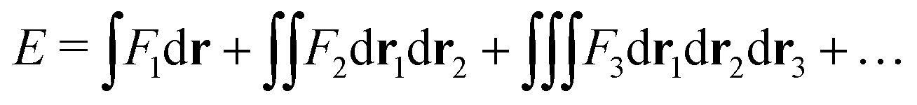 | (26) |
| F1 ≡ F1(r, ρ(r), ∇ρ(r),…), | (27) |
| F2 ≡ F2(r1,ρ(r1),∇ρ(r1),…, r2,ρ(r2),∇ρ(r2),…), | (28) |
The LDA and GGA functionals correspond to the first term of the expansion in eqn (26). Examples of the second-order term (“two-point functionals”) are the naive Hartree energy and the vdW-DF energy functional of Langreth, Lundqvist, and co-workers.395
The expansion in eqn (26) may be relevant in the quest for explicit density functionals for the kinetic energy, a topic that has seen revived interest recently in the context of orbital-free DFT. Here, however, I will confine my remarks to the theory of van der Waals interactions (London dispersion),396 with which I am more familiar.
For dispersion interactions, the second-order term in eqn (26) has already had considerable success via the vdW-DF functional395 and its extensions.397 The third-order term would be needed, for example, for a strictly explicit density functional to capture the Axilrod–Teller–Muto interaction – that is, the van der Waals interaction between three atoms, taken beyond the summed interaction between pairs of atoms).
It has been known for some time that widely-spaced low-dimensional metals have van der Waals interactions that are qualitatively different from those between nonmetallic structures with a similar geometry;398–400 for some discussion, see Chapter 11 of ref. 396. Recently, it has been found that this specific metallic van der Waals physics is important beyond the asymptotic region, indeed right down to contact, for metallic nanotubes and doped graphene sheets. This behaviour was captured by calculations401 of the electron correlation energy in direct RPA (dRPA). Methods like dRPA start from an electronic band-structure calculation and are thereby sensitive to the presence or absence of a zero HOMO–LUMO gap (band gap). I fear that a very high order in the functional expansion in eqn (26) might be needed to capture such physics. I wonder, though, whether one could use a close examination of the ground-state electron density in the tunnelling region between atoms, in order to recognize the band gap. Certainly, this region determines the overlap (tunnelling) energy integral t in the tight-binding description of electronic band structure. In that case, perhaps the first few terms on the right-hand side of eqn (26) might be sufficient.
3.6 What is the role of symmetry breaking/restoration for DFAs?
It is only via symmetry breaking that the interaction of the electrons with the nuclei can be regarded as a static external potential. In a symmetry-unbroken wave function for electrons and nuclei, all potentials are internal and all effects are correlations. The quantum theory of measurement requires a symmetry-broken or classical observer. The measured antiferromagnetism of solids is a physical symmetry breaking: a fluctuation or correlation that persists for a long time even on the human scale.404 Thus, condensed matter physicists tend to be more comfortable with symmetry breaking than many quantum chemists are. While the symmetry of the ground state of a finite system remains unbroken when averaged over an infinite time interval, the time interval over which the symmetry remains broken in a fluctuation can grow rapidly as the spatial extent of the system grows. The macroscopic world as we perceive it is symmetry-broken and classical.
Apart from the reasons mentioned in contribution (3.6.2), further efforts to avoid symmetry breaking might be worthwhile in order to obtain potential-energy surfaces without kinks.
In the Kohn–Sham treatment, we then have a choice: (i) we can require the spin density to be identical in the Kohn–Sham and true electronic systems. This choice amounts to a spin-polarized Kohn–Sham calculation with a Kohn–Sham Hamiltonian operator that is no longer rotationally invariant in spin space. Spin is then no longer a good quantum number for the Kohn–Sham determinant – that is, spin poisoning occurs. (ii) Alternatively, we can require the total density but not the individual spin densities of the Kohn–Sham system to be identical to the true electronic system. The Kohn–Sham Hamiltonian operator then remains rotationally invariant in spin space and we get identical spin-up and -down orbitals. As a result, the orbitals and the Kohn–Sham wave function can be chosen to have well-defined spin but the individual Kohn–Sham spin-up and -down densities are no longer identical to those of the true electronic system. In practice, approach (i) is typically taken – however, approach (ii) is equally correct from a formal perspective, a point Walter Kohn made from time to time.
A similar choice can be made with respect to symmetries in real space. In open-shell atoms, for example, one can either require that the total density or the spin densities for the Kohn–Sham system and true electronic systems are identical or require that only their totally symmetric (i.e., spherical) real-space components are identical.409 Depending on the choice made, the Kohn–Sham Hamiltonian either has a symmetry lower than the spherical symmetry of the true Hamiltonian in real space or is spherically symmetric in real space like the Hamiltonian of the true electronic system.
These choices, leading to different but formally correct Kohn–Sham approaches, must be distinguished from symmetry breaking of the type observed in a dissociating hydrogen molecule. The Kohn–Sham Hamiltonian has been shown to exhibit at least the symmetry of the total density or spin density of the true electronic system.409 In the dissociating hydrogen molecule, the true density is non-spin-polarized at all distances. Therefore, an exact spin-polarized Kohn–Sham calculation always reduces to the non-spin-polarized case. If this reduction does not occur, then it is an artefact of the employed approximate exchange–correlation functional, pointing to a shortcoming in the description of static correlation.
Finally, it should be pointed out that symmetry-breaking contributions in the Hamiltonian of the real system necessarily lead to corresponding terms in the Kohn–Sham Hamiltonian. Spin–orbit interactions, for example, require from a formal point of view the presence of terms in the Kohn–Sham potentials that couple to spin or magnetization currents.410 In practice, these terms are often neglected. It is interesting to note that, from a formal point of view, terms in the Kohn–Sham potential that couple to noncollinear spin are not required in the presence of spin–orbit interactions.410
For instance, for a f7 → d1 transition in a lanthanide compound (here europium), the GGA Kohn–Sham MO occupations corresponding to the 4f6d1 configuration is 6/7e for the (7) MOs strongly localized on the Eu/4f orbital, and 1/5e for the (5) MOs mostly localized on the Eu/5d orbital. See, for example, the case of the Eu(η9-C9H9)2 complex, for which the 30![[thin space (1/6-em)]](https://www.rsc.org/images/entities/char_2009.gif) 030 multiplet energy levels have been calculated.413
030 multiplet energy levels have been calculated.413
So spin-contaminated (as traditionally computed) Kohn–Sham DFT or TDDFT solutions might, in fact represent the correct spin densities of the spin-pure correlated many body wave functions – for example, an open-shell doublet radical (such as CH3) in which the unpaired electron has alpha spin, is known to have areas with an excess beta-spin density.414 This cannot be reproduced by a spin-adapted (ROHF) Kohn–Sham determinant (which only allows for an excess alpha density), hence suggesting that a spin-polarized Kohn–Sham determinant provides a more appropriate description.
Because we do not know how to compute the S2 value in DFT, we should formulate this question – whether or not we have unphysical symmetry breaking – in terms of finding molecular properties that could report on it. The same concerns apply to spatial symmetry breaking. One example of how one may approach this problem is a charge-transfer system, such as (He)3+ or the charged ethylene dimer. Charge localization is very sensitive to Hartree–Fock-like symmetry breaking and also to the SIE. The comparison of charge localization patterns against high-level reference data can inform us whether symmetry breaking is real or artificial; some useful examples can be found in ref. 415.
3.7 What is the role of ensemble methods for DFAs?
Thermal ensembles are rather different to the other types of ensembles. The following discussion thus focuses on other types of ensembles, which give insight into spectroscopic properties of electronic systems, like fundamental and optical gaps.
Despite representational issues in some systems, there are a wide variety of problems for which ensembles can be described cleanly, and for which mappings are one-to-one.424 In such cases, key ensemble functionals may be defined as,6,8
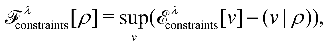 | (29) |
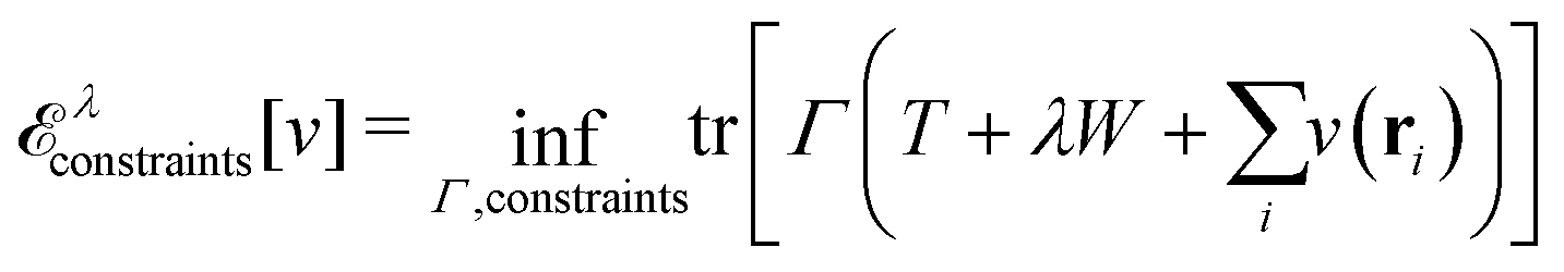 | (30) |
![[scr T, script letter T]](https://www.rsc.org/images/entities/char_e533.gif) s[ρ] := s[ρ] := ![[scr F, script letter F]](https://www.rsc.org/images/entities/char_e141.gif) 0[ρ], 0[ρ], ![[scr E, script letter E]](https://www.rsc.org/images/entities/char_e140.gif) Hxc[ρ] := 1[ρ] − 0[ρ], Hxc[ρ] := 1[ρ] − 0[ρ], | (31) |
s and Hxc serve the same role as in conventional DFT. “Constraints” are henceforth implied by the use of calligraphic letters.
Eqn (31) defines an ensemble Kohn–Sham system with orbitals obeying,
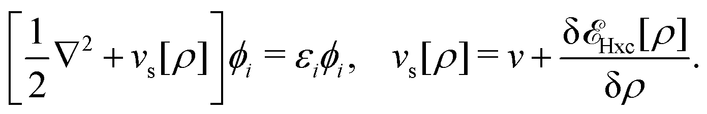 | (32) |
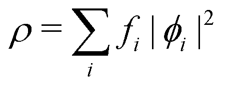 , is defined using orbitals with allowed fractional occupation factors, fi, that reflect the nature of the ensemble. Ensembles are thus amenable the same machinery as standard DFT – that is, by approximating Hxc[ρ] and then finding a set of self-consistent orbitals and density. Accommodating ensembles in Kohn–Sham DFT not only extends approximations to new problems (like excited states), but can also remedy deficiencies in standard approximations.425,426
A major difficulty in treating ensembles is that the minimizing wave functions and ensembles are not guaranteed to be unique and cannot be used explicitly to define functionals – the “nonuniqueness disaster”.427 This is related to issues raised in contribution (3.7.1). One must thus resort to more foundational relationships to further break Hxc into useful pieces that may then be approximated. A rigorous separation into Hartree–exchange and correlation terms is achieved by using,
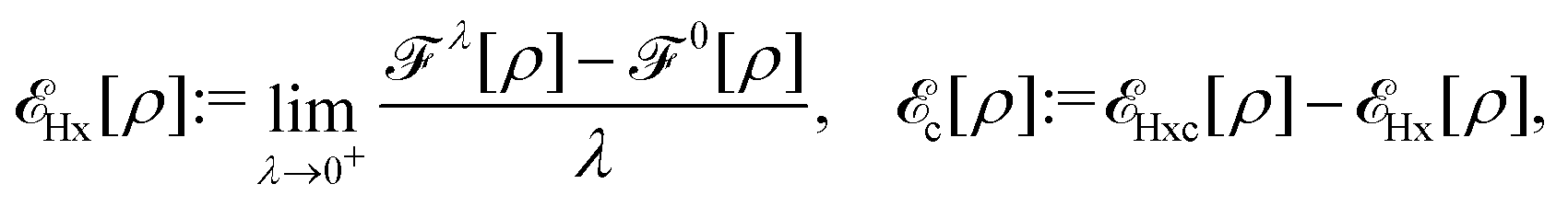 | (33) |
FDTH[ρ] and exchange term FDTx[ρ] using the fluctuation-dissipation theorem.428 The resulting orbital functionals reduce to their usual definitions in pure states. Hybrid functionals formed on these orbital functionals (e.g., by using s + FDTH + αFDTx, where α is a HF mixing parameter) may be defined using ensemble generalized Kohn–Sham theory.175
An additional challenge in ensemble DFT is that the correlation energy is more complicated than its standard (pure-state) DFT counterpart. Firstly, because it must address multiple states at once. Secondly, because it contains density-driven (DD) correlations,429 which are a consequence of the fact that Kohn–Sham states reproduce the correct total density, but not the correct densities of the individual interacting states included in the ensemble. Gould and Pittalis defined DD correlations in special types of ensembles.429 Fromager then provided a rigorous general scheme for understanding DD correlations.430
The discussion that follows focuses on the latter type of ensembles, which we could refer to as “pre-defined” ensembles. Indeed, unlike in thermal DFT,431,432 the ensemble weights ξ = (ξ0,ξ1,…, ξI,…) that are assigned to each state within the ensemble will always be known before the ensemble DFT calculation is carried out. They are chosen (in principle, arbitrarily) and fixed. In other words, in the exact theory, the Hohenberg–Kohn theorem is established for a given ensemble or, equivalently, for a given set ξ of weight values. The one-to-one correspondence between local potentials and ensemble densities relies on the extension (from pure ground states to ensembles) of the Rayleigh–Ritz variational principle,421,423
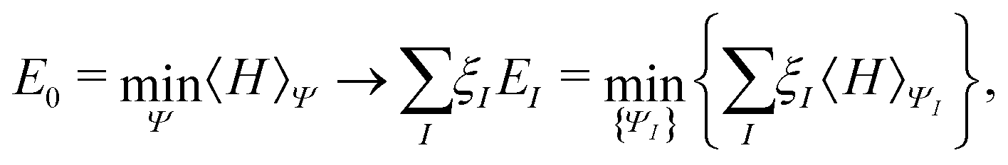 | (34) |
| Hxc[ρ] ≡ EξHxc[ρ] | (35) |
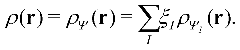 | (36) |
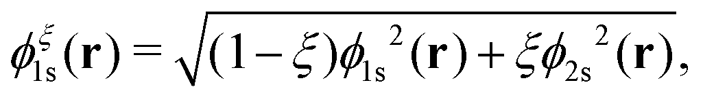 | (37) |
In the general many-electron case, the ensemble Hxc functional needs to know if it has to compute the Hxc energy of a pure ground state or of an ensemble consisting of ground and excited states, hence the ξ dependence in EξHxc [ρ]. The extraction of excitation energies from an ensemble DFT calculation reveals the importance of this weight dependence.422,423,434,435 In particular, it has been shown that ensemble density-functional weight derivatives ∂EξHxc[ρ]/∂ξI are directly connected to the derivative discontinuities that the Hxc potential exhibits when a given excited state is incorporated into the ensemble.436–438
In DFT for (canonical, for simplicity) thermal ensembles,431,432,439 the ensemble weights are controlled by a single parameter – the temperature or, equivalently, the inverse temperature β. In thermal DFT, the variational principle is extended to the total (Helmholtz) energy, which contains an entropic contribution:
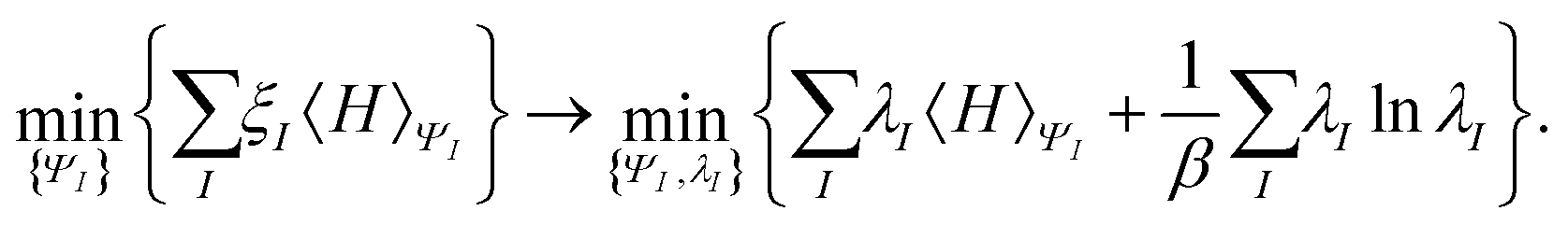 | (38) |
are energy dependent. Therefore, they are unknown when the calculation starts. Moreover, even though both interacting and noninteracting Kohn–Sham systems are described at the same temperature and share the same (ensemble) thermal density, their ensemble weights are different, simply because Kohn–Sham energies do not match the true interacting ones.
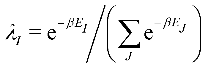
With these major differences in mind, the discussion on ensemble DFAs that follows essentially applies also to thermal DFT. The ensemble-weight dependence of the Hxc functional simply reduces to a temperature dependence.
Hx427 and then break it down into FDTH and FDTx428 has offered insights into adapting existing approximations to ensembles – because the exact-exchange functional of more complex excitations can obey combination rules that relate it to simpler pure-state systems for which approximations already exist. I showed that using exact-exchange relationships for ensembles allowed ensemble DFT to outperform the ΔSCF and TDDFT methods using the same DFAs.442 This success has been partially transferred to double excitations.443 Despite improvements from using the ensemble version of the on-top pair density Π(r,r) given for pure states in eqn (25),443 how to effectively reuse existing correlation DFAs remains an outstanding problem. It should be noted, however, that these DFAs require solution of orbital equations.175
Note that the approaches discussed above focus on modelling the Hx functional and state-driven correlations.429,430 Failure to include DD correlations in ensemble DFAs leads to “DD correlation errors” that are avoided in pure-state DFT. Gould introduced an extrapolation scheme to approximately avoid DD correlation errors.424
(1) Self-consistent ensemble DFT calculations still lack a well-defined computational protocol (usual or generalized Kohn–Sham schemes, OEP-type algorithms, CASSCF-type orbital optimization techniques, etc.). How best to correct the ghost-interaction error at an affordable cost is also an open question.444
(2) In GOK DFT,421 one is supposed to know in advance the energy ordering of the excited states, which is far from being straightforward.
(3) Different flavours of ensemble DFT are used depending on the type of excitations targeted. In this context, a unified theory for charge and neutral excitations would be desirable in order to be able to compute both the fundamental and optical gaps from a single calculation.
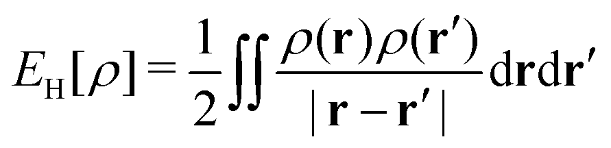 | (39) |
 | (40) |
 | (41) |
Nevertheless, it is possible to tackle the problem differently. Indeed, an orbital-dependent Hartree-only density functional can be defined using Lieb's maximization (see eqn (29)) and the following approximate expression for the potential-functional ensemble energy:438
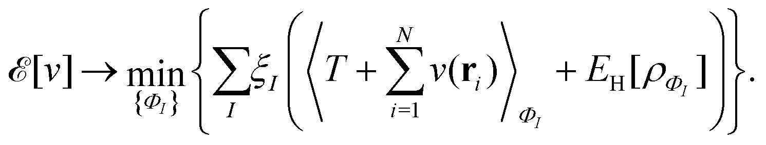 | (42) |
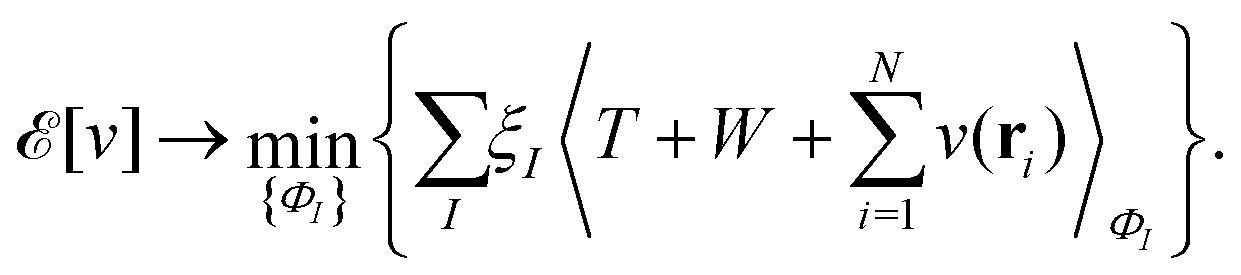 | (43) |
Electron correlation can be introduced (approximately) into the theory by recycling the regular (weight-independent) ground-state correlation functional Ec[ρ] as follows:
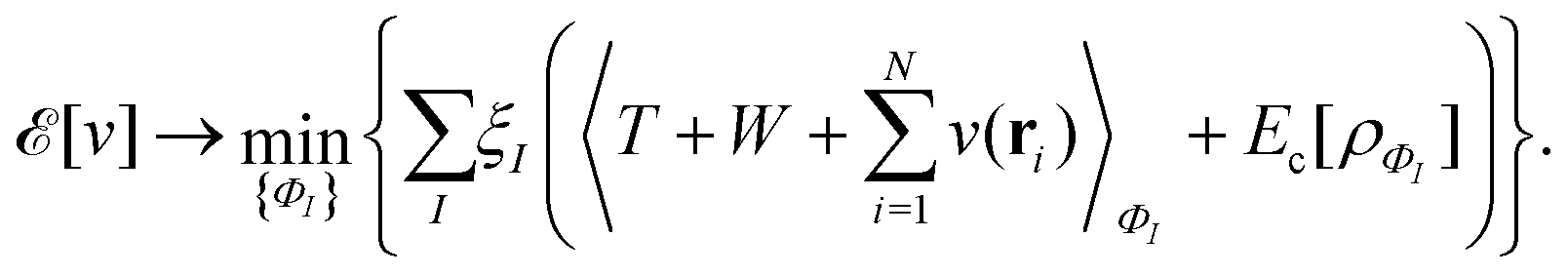 | (44) |
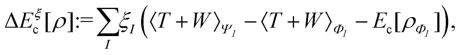 | (45) |
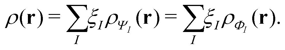 | (46) |
Let us give further insight into the approximation of eqn (44). From the more explicit expression
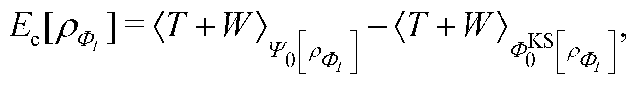 | (47) |
 | (48) |
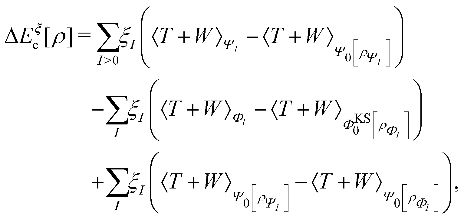 | (49) |
Let us finally mention that ensemble DFT does not give a direct access to response properties such as oscillator strengths or to Dyson orbitals (in the case of N-centred ensemble DFT423). The extension of Görling–Levy perturbation theory133,449,450 to ensembles should probably be explored for that purpose.
Recently, my coworker Dr Yangyi Lu and I proved that MSDFT is an exact DFT in the subspace ![[Doublestruck V]](https://www.rsc.org/images/entities/char_e179.gif) N spanned by the lowest N eigenstates of the Hamiltonian.459 It is proved (1) that the Hamiltonian projected onto N is a matrix functional H[D(r)] of the multistate matrix density D(r) and (2) that variational minimization of the multistate energy, EMS[D] = trV[S−1H(D)], gives the exact energies and densities of all N eigenstates. The second theorem corresponds to an extension of the Theophilou variational principle for the whole subspace460 in terms of H[D(r)], ensuring that the energies and vectors of individual states are obtained simultaneously. In these expressions, D(r) is a matrix of electron densities and transition densities of a set of basis states that represent the ensemble density ρV(r) = trV[S−1D(r)] of the subspace N, where S is the overlap matrix of the basis states; D(r) is not to be confused with the one-electron density matrix.
N spanned by the lowest N eigenstates of the Hamiltonian.459 It is proved (1) that the Hamiltonian projected onto N is a matrix functional H[D(r)] of the multistate matrix density D(r) and (2) that variational minimization of the multistate energy, EMS[D] = trV[S−1H(D)], gives the exact energies and densities of all N eigenstates. The second theorem corresponds to an extension of the Theophilou variational principle for the whole subspace460 in terms of H[D(r)], ensuring that the energies and vectors of individual states are obtained simultaneously. In these expressions, D(r) is a matrix of electron densities and transition densities of a set of basis states that represent the ensemble density ρV(r) = trV[S−1D(r)] of the subspace N, where S is the overlap matrix of the basis states; D(r) is not to be confused with the one-electron density matrix.
The multistate matrix density D(r) can be sufficiently represented by N2 nonorthogonal (necessary) determinants.459 In a departure from Kohn–Sham DFT for the ground state, we introduce in MSDFT an “active space” of N interacting states {ΦA; A = 1,…, N}, each of which is written as a linear combination of N2 nonorthogonal determinants, 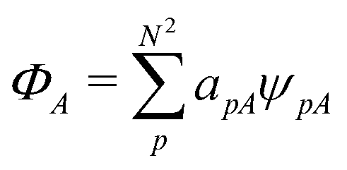 , to completely represent D(r) of the real (fully interacting) system. Its matrix elements are computed from one-electron orbitals {χApj(r)} in the manner
 | (50) |
Analogous to the ground-state DFT, we can define a Lieb-like subspace energy functional
 | (51) |
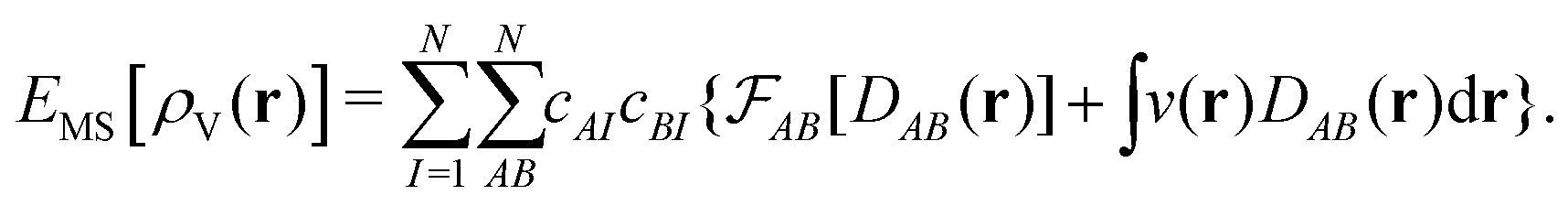 | (52) |
N are thus simultaneously determined.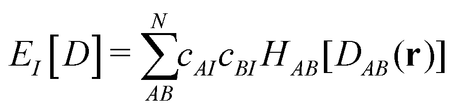 | (53) |
N is given by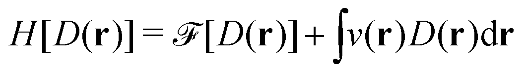 | (54) |
[D(r)] is the universal matrix functional, whose elements in terms of one-body orbitals are| [D(r)] = TMS[D(r)] + EHx[D(r)] + Ec[D(r)] | (55) |
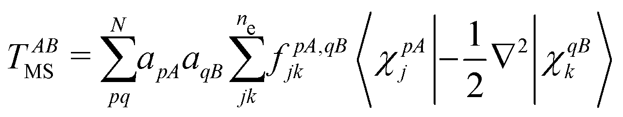 | (56) |
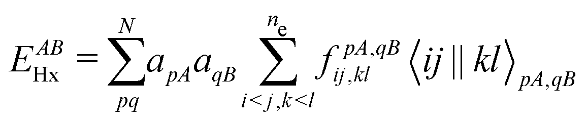 | (57) |
Notice that I have introduced a new class of density functional, the transition density functional (TDF) EABc[D(r)] between states A and B.458 The physical interpretation of the TDF is the dynamic correlation contribution to the electronic coupling between two basis states.457,458 Although the functional form of the TDF is not known (similar to the exchange–correlation functional in Kohn–Sham DFT), in special cases such as spin-coupling interactions, it can be determined with the constraint of spin-multiplet degeneracy with the high-spin state determined separately using Kohn–Sham DFT.457,458 Obviously, as in Kohn–Sham DFT, EABc[D(r)] also includes the corresponding residual kinetic energy not expressed in the orbital term.
One way to construct the multistate active space is to use constrained Kohn–Sham determinants for the states of interest. These non-Aufbau configurations can be optimized via a ΔSCF procedure,461 or by the targeted orbital optimization method.462 If we do not simultaneously optimize {cAI,apA} in eqn (52), the orbitals in each determinant will be separately optimized, and they are generally nonorthogonal. Then, the procedure is equivalent to nonorthogonal state interaction (NOSI), a convenient approximation to the full MSSCF solution.454,455 In this case, one first carries out the optimization of each determinant configuration as a constrained Kohn–Sham DFT calculation.455,463 Then, this is followed by a single step of diagonalization of the Hamiltonian matrix functional (eqn (54)), with the approximations for the off-diagonal elements HAB given in ref. 454, 455 and 457 to yield the energies of the adiabatic states. Consequently, all adiabatic states in the subspace, including the ground state, are treated on an equal footing in the course of minimizing the multistate energy functional.458
Since state interactions are explicitly included in the active space that defines the multistate energy, the effect of interference highlighted in contribution (3.7.1) is naturally included in MSDFT.
3.8 What has DFT told us about the real world?
However, this is not the main lesson that DFT has taught me about the “real world”. I participated in (and survived) the struggle of a small number of scientists to convince the overwhelming majority of theoretical chemists that density-functional calculations could play an important role in chemistry. This struggle (from the mid-1970s to the breakthrough to general acceptance in the early 1990s) was against a conservative community that, with few exceptions, did not hesitate to “vilify” (Baerends, personal communication), ridicule, or ignore a development that everyone now knows was in its own interests. Such long-running rejection of unfamiliar ideas is certainly not unique in science, but I hope that it will not be repeated in the density-functional community.
“1 am. A faint knock on the downstairs door. Or was it? Then the unmistakable thump of a heavy boot against the door and the crack of the door jamb as it shattered. Had his sordid past caught up with him? The interrogation would be swift and on the spot. Where did that wooden chair come from? And the bare light bulb slowly swaying above it? Whose face was that, almost invisible behind the glare? Inquisitor: Are you now or have you ever been a member of the Xalpha party? Mild-mannered respectable density-functional-theory practitioner (MMRDFTP): What? (Where had he heard that voice before?) Inquisitor: Are you now or have you ever been a member of the Xalpha party? MMRDFTP: I’m a Mild-mannered respectable density-functional-theory practitioner (MMRDFTP). What do you mean by breaking into my house in the middle of the night and hauling me out of bed like that? I was just in the middle of a great dream about an exchange–correlation functional that had the right asymptotic form and took care of dispersion seamlessly. Could have done excited states too, and eminently parallelizable. And now I’ve forgotten what it looked like”
Perhaps this has something to do with the “real world”.
And to make it clear: wave-function-based theory should be used wherever it can be used. But this is exactly the point. DFT is applied for large systems because of its low computational scaling law, O(n3), with the number of particles involved n, and where wave-function-based theory has (and in future will still have) real problems – for example, in describing electron correlation for strongly correlated and metallic systems. The electron-correlation problem for metallic systems in wave-function-based theory was already pointed out in early days by Fulde.466 Here, DFT gave us many useful results of the “real world” where ab initio theory is just not able (yet) to do the same job. It has become therefore an invaluable tool for materials science, solid-state physics, and the simulation of biomolecules.
What is perhaps a bit annoying (at least to me) are the “quick fixes” applied to DFT when one does not get reasonably accurate results – I just mention here the better description of electron pairing due to the on-site Coulomb repulsion by the use of the Hubbard term in DFT + U.467,468 On the other hand, many-body theory can be used successfully within a DFT formalism as the many applications in solid-state physics show – for example, by using GW and Bethe–Salpeter theory leading to quite accurate solid-state properties. So the two worlds come together somehow.
Confirmation. Sometimes experimental findings can be conflicting or controversial, owing to sample quality, complexity of measurement, difficulty of interpretation, or all of the above. “Reproducing” the experiment on the computer, using DFT, allows theorists to weigh in on such controversies.
Interpretation. Often the experimental result is beyond dispute, but it is poorly understood. With DFT, we can easily test for the effect of, for example, adding, moving, or removing an atom; we can examine the role of transition states and metastable states; we can assess what individual (Kohn–Sham) electron orbitals do and more. By doing so, we can explain experiment. The same tasks would range from the exceedingly difficult to the a priori impossible if attempted experimentally.
Prediction. Suggesting new mechanisms and properties before they have been examined experimentally, or indeed even suggesting new useful molecules or materials before they have been synthesized, once seemed like a distant “holy grail”. It is a testament to the quality of modern DFAs that such predictions are becoming increasingly successful.
3.9 What is the status of DFT-based tools for interpretation of chemical phenomena?
The aim of conceptual DFT was clarified at a conference in Changsha City, China in 2018, attended by almost all of the most influential workers in the field, and formulated in the above mentioned status paper as “to develop a nonempirical, mathematically and physically sound, density-based, quantum-chemical theory for interpreting and predicting chemical phenomena, especially chemical reactions”.475 This aim should be realized with a philosophy based on three fundamental precepts: observability (our understanding of chemical observations should be based on quantum-mechanical observables – in particular, the energy, the density and their derivatives); universality (the results should not depend on the type of calculations) and mathematical rigour (aiming at a well-defined mathematical framework).
Based on these precepts, conceptual DFT has introduced a number of molecular reactivity descriptors, mostly response functions or descriptors derived from the E(N) curve, that – either alone or in combination with the electronegativity-equalization principle, the hard/soft-acid/base principle, the maximum-hardness principle, or the minimum-electrophilicity principle, for example – have served as valuable tools for the interpretation of experimental and theoretical (computational) data for a wide variety of reactions. Its scope comprises “generalized” acid–base, complexation and redox reactions and a multitude of “classical” organic reaction types including pericyclic reactions, with substrates varying from inorganic to organic and organometallic molecules, to polymers and the solid state. The success of conceptual DFT in pervading a broad range of chemical subdisciplines – from inorganic, organic, and organometallic chemistry to biochemistry and materials chemistry – can be described as getting “insight from numbers”, experimental or theoretical.
Pitfalls and shortcomings are still to be coped with, however, both on the more fundamental issues (e.g., the nature of the E(N) function and the issue of differentiability, the convergence of the E = E[N, v] perturbation series in N and v) and on more applied aspects (e.g., the delineation of the scope of the various principles) before the next step, from interpretation to prediction, can safely be taken; see Section 4.8.
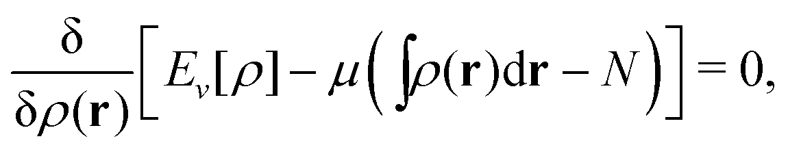 | (58) |
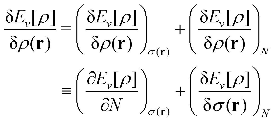 | (59) |
The typical solution in the theory of variations under constraints is to choose some extension of the functional into the domain where it is not defined. This extension is essentially arbitrary, the only requirement is that the extension obeys continuity properties so that the derivative exists. At this point, the Lagrange multiplier, which is the force of constraint keeping the density at integer N, is undetermined. It is determined by the chosen extension of E[ρ] into the noninteger domain. This is not a problem, it is directly related to the well-known gauge freedom of the Kohn–Sham potential, to which an arbitrary constant may be added.476 In a widely cited paper by Parr et al.186 (see also contribution (2.5.3)), the Lagrange multiplier μ has been described as “a characteristic constant for a system”, but without any proof or arguments. This contradicts the essential arbitrariness of the constant μ, and therefore of ∂E/∂N. Atoms and molecules have an ionization energy and an electron affinity – there is no additional physical quantity μ = ∂E/∂N.
The best known choice for extension of Ev[ρ] into the noninteger domain is the one of ref. 18 – namely, forming an ensemble of the ground-state density matrix of the N-electron system with either the density matrix of the ground state of the (N + 1) system or the ground state of the (N − 1) system. This procedure leads to piecewise linear energy behaviour. This choice precludes application of the Euler–Lagrange variation method because the derivative ∂E/∂N does not exist (is discontinuous at the integer point). More extensive discussion of these matters is given in ref. 478.
The perturbed energy can be analysed as a contribution from excited configurations, whose importance may be estimated by their oscillator strengths. In most cases, it appears that only a limited number of excitations contribute significantly to the overall response to the perturbation, suggesting that chemical reactivity can be predicted by analysing the reshuffling of electron density upon excitation.482 The stabilization energy due to interaction between the polarization density and the electrostatic potential δv(r) is given by
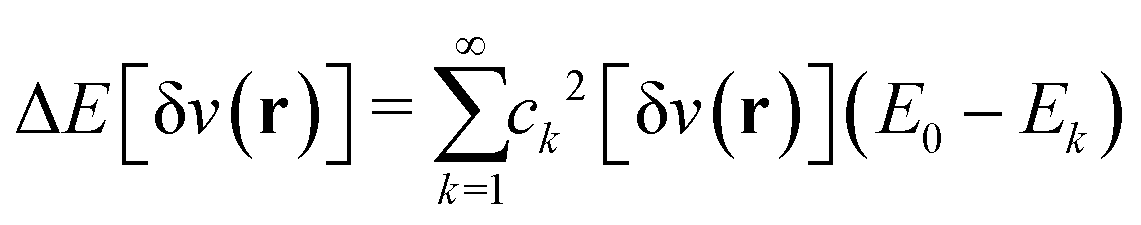 | (60) |
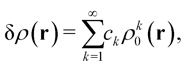 | (61) |
From a link between conceptual DFT and statistical thermodynamics, it has been shown that the perturbation energy due to intermolecular electrostatic interactions can be understood in terms of effective work and heat exchange,484 the first-order correction  being the effective work and the second-order correction in eqn (60) being the heat exchange. A polarization entropy and a polarization temperature can also been defined by this analogy. Therefore, using the external electrostatic potential as a probe and the polarization energy, entropy, and density as electronic responses, one can get qualitative and quantitative insight into the reactivity and the selectivity of molecular fragments.483
4 The Future of DFT and DFAs
4.1 What are the important lines of development in DFT and for DFAs?
This bottleneck problem has been efficiently resolved in the CASΠDFT488 and ELS+ (the extension of the above mentioned ELS method)64 methods, which share the following master formula for the electronic energy:
 | (62) |
 | (63) |
| EMC-NCFT[ψMC] = EMCclass + Enc[f[ψMC]] | (64) |
There are two main issues that should be addressed in the future, if MC-PDFT is to become a routine method for multireference systems:
1. How should one choose reference wave functions for these calculations and make them affordable for extended systems? Instead of using the CASSCF wave function, one can use RASSCF or generalized-active-space SCF (GASSCF) wave functions or DMRG wave functions.497 Related to this challenge is the task of automating active-space selections to make these methods more user friendly.
2. The second direction of development is towards the functional form. Currently, functionals are borrowed from the Kohn–Sham world, but specific functionals for this theory should eventually be developed. One possibility is to develop multiconfigurational density-driven functional methods that correct the classical or total energy of a multiconfigurational wave-function method through the use of a machine-learned functional.492
The separation of the electron–electron repulsion into a long-range (lr) part and a short-range (sr) part is usually achieved with the error function erf(−μr12) where μ is an interaction-strength parameter. By means of the AC, one obtains a continuous range of possible DFA models defined by different values of μ ≥ 0. In particular, one obtains Kohn–Sham DFT for μ = 0 and pure wave-function theory (WFT) for μ →∞; the AC from μ = 0 to μ = ∞ thus provides an alternative path to Kohn–Sham DFT.
The more interesting case is to use the AC from a partially interacting system at finite μ > 0 to μ = ∞. One then obtains a hybrid lrWFT–srDFT model, which, for a sufficiently large μ, can describe nondynamical long-range correlations adequately and also give correct spin symmetry of open-shell molecules498 by means of a multideterminant reference wave function. This approach is much simpler than attempting to describe them with a complicated Kohn–Sham DFA functional based on a single determinant. On the other hand, the dynamical short-range correlation effects can be described efficiently with a semilocal srDFT functional connecting to a Kohn–Sham DFT functional in the μ = 0 limit.
In the hypothetical case of short-range exact density functionals and long-range FCI wave functions for any μ value, the total energy would be the same for all μ values. The idea is to use the μ value for which the least computational work is needed to obtain good-quality energies and properties.
The computationally most efficient lrWFT–srDFT model will be for the smallest μ value for which long-range and spin correlations can be described to the desired accuracy, as this leads to the most compact lrWFT part with the smallest number of active orbitals. By comparison with accurate wave-function calculations, it has been found that a value around μ = 0.4 can be considered universally applicable for valence properties of singlet molecules.499–501 Preliminary investigations of transition-metal complexes indicate that a value around μ = 1.0 may be needed to describe their spin correlation sufficiently well.502
A particularly promising choice for the lrWFT part is to use the variational multiconfigurational self-consistent field description, leading to an lrMCSCF–srDFT (MC–srDFT) model. Because it is variational, the MC–srDFT model can also be used for molecular response properties, just like TDDFT in Kohn–Sham DFT – not only for excitation energies and transition moments, but in general for optical, electrical, and magnetic perturbations. For molecules with strong nondynamical correlation, the kinetic energy will be better described with the MC–srDFT model than with Kohn–Sham-DFT, thus a smaller kinetic-energy correction needs to be described by the correlation functional.
Note also that the MC–srDFT approach can be used not only for electronic ground states, but also in state-specific models for excited electronic states of any spin multiplicity and spatial symmetry.
The most successful practical incarnation of this idea has been based on another highly successful idea – namely, that of range-separated hybrid functionals.106,504 These functionals can exhibit an asymptotically correct long-range (free91 or screened505) Coulomb potential, while retaining a useful balance between exchange and correlation in the short range. The range-separation parameter is then tuned, per system, by enforcing the ionization-potential theorem18 (or variants thereof). The approach has been successful in overcoming issues considered very challenging for DFAs, notably the infamous band-gap problem506,507 and the prediction of charge-transfer excitation energies,508,509 through systematic elimination of derivative discontinuity errors. Importantly, this approach restores the physical picture of single- and two-quasi-particle excitation thresholds, by reliably predicting them from the HOMO–LUMO eigenvalue difference of a DFT calculation and the lowest eigenvalue of a TDDFT calculation, respectively, using the same exchange–correlation functional.91 Extensions of these ideas can be expected to continue to play a role in DFT applications to spectroscopy.
While many approaches to reducing delocalization error have been proposed, none is a panacea. Typically, one can reduce delocalization error through a (frequently range-dependent) mixing of local, DFA exchange and nonlocal, Hartree–Fock exchange. However, the optimal mixing is known to be highly system and size dependent.513,514 Development of a practical and universally applicable DFA with minimal delocalization error remains an outstanding challenge and would represent a significant advance.
There are various ways to go beyond the RPA. Highly promising are σ-functionals,515,516 which are technically closely related to the RPA but formally rooted in many-body perturbation theory along the AC. Methods using σ-functionals are distinctively more accurate than RPA-based or conventional functionals – they reach chemical accuracy for main-group chemistry and treat noncovalent interactions accurately.
While some methods based on the ACFD theorem are computationally expensive, this is not at all true for functionals within the RPA or for σ-functionals. These are typically evaluated in a post-SCF way, ideally using orbitals and eigenvalues from hybrid DFT methods. In this case, the post-SCF calculation of the total energy using the RPA or the σ-functional requires less computational time than the preceding hybrid calculation and thus can be easily carried out routinely.
There is much room for further developing correlation functionals based on the ACFD theorem and these functionals open up a new area for DFT – the field of highly accurate electronic-structure calculations, so far dominated by wave-function methods like the hierarchy of coupled-cluster methods.
A simple replacement of standard PT2 by more sophisticated correlation models from wave-function theory does not seem to lead to a notable improvement in accuracy despite the higher cost.518 Some recent efforts to develop efficient models that go beyond PT2 for double-hybrid approximations have led to some encouraging schemes for further progress.519–522
These advantages extend also to TDDFT computations of various types of excitations, including core, valence, and Rydberg excitations, with particularly good performances for triplet excitations.530,531 In general, LHs give extra flexibility to balance minimal self-interaction or delocalization errors in some regions of space with the simulation of left–right correlation in bonds. LHs can be further extended in various directions by combining with range separation (e.g., local range separation532–534 and range-separated LHs535,536), by adding dispersion either via correction terms or via nonlocal van der Waals functionals, potentially by adding nonlocal rung-5 correlation contributions, or by adding corrections for strong correlation.
For transition-metal systems, the situation is more complex and less developed than for main-group systems.539–541 Large transition-metal test sets with accurate reference data are urgently needed. It is not merely important for benchmarking Kohn–Sham DFAs, but also fundamentally important for understanding the limitations of current Kohn–Sham DFAs for strongly-correlated systems as mentioned in contribution (3.4.1), since transition-metal systems often have a strong multireference character.
The recent TASK545 and modified (mTASK)546 meta-GGA DFAs are energy functionals developed explicitly for band gaps. Both DFAs excelled in accuracy for band gaps of some important but limited test sets of bulk solids and two-dimensional materials. However, more tests should be done in order to reveal the strengths (and limitations as well) and applicability of these meta-GGAs. With more information, the TASK and mTASK approximations can compete with available hybrid functionals such as the HSE06 functional in accuracy, at a more favourable computational cost. Such applications for the fundamental band gap could initiate the development of exchange–correlation kernels for optical response properties constructed from these meta-GGA functionals. This latter possibility is an obvious advantage of DFAs that possess functional derivatives. The static exchange–correlation kernel from a DFA is its second functional derivative with respect to the density, which needs to exist for this approximation.
The real challenge is to develop KEDFs that can describe molecules and transition metals (similar problems will exist for f-block elements). The inherent angular momentum dependence of the electron distributions – captured by orbitals but not by densities – makes KEDF development for far-from-uniform densities truly a grand challenge. Self-consistent all-electron calculations, without pseudopotentials/effective core potentials, are also a huge challenge due to the same issues. We have shown how difficult this is to accomplish in several papers, where we can achieve small wins but easily break our models as well; see, for example, ref. 555–559, as I believe strongly – as discussed later in contribution (4.4.4) – in the value of publishing failures to gain insight into how to advance the field.
A crucial point for the orbital-free DFT agenda that often goes undiscussed is to get rid of the orbital dependence in DFAs. This is the antithesis of much of the activity in the quantum chemistry community, as much of the discussion in this roundtable confirms. We have made considerable progress on de-orbitalization of meta-GGA DFAs542,543,563 by inclusion of a dimensionless ∇2ρ dependence, though the success of that approach is quite dependent upon the numerical stability of the parent meta-GGA DFA.
Our single-point KEDFs have no problems converging and yield properties in good agreement with Kohn–Sham DFT for the usual materials – simple metals – but again, we can easily break them. Just study a vacancy or an alloy, both of which by contrast are handled well by our 1999 nonlocal WGC KEDF.566,567 Our 2015 pointwise analysis of our single-point KEDFs compared to the WGC KEDF indicates at least some of what is needed to help improve such single-point KEDFs565 – namely, reproducing of the inherent multivaluedness of the non-von-Weizsäcker component of the GGA enhancement factor when plotted against the reduced density gradient. The WGC KEDF, remarkably, does so, indicating yet another fundamental reason it is so accurate for simple metals.
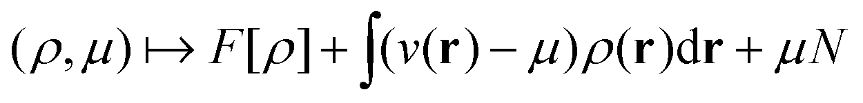 . An interesting finding is that more complicated GGA-type functionals often show an erroneous nonconvex behaviour for the model
 ![[T with combining tilde]](https://www.rsc.org/images/entities/i_char_0054_0303.gif) s[ρ] (where tilde indicates an approximate quantity). As a result, many solutions (rather than one solution) to the Euler–Lagrange problem with a given particle number N are found. Since Ts[ρ] is the noninteracting limit of F[ρ] and since both functionals are convex with respect to the density variations, it would be interesting to explore techniques to impose convexity on approximate s[ρ] and
s[ρ] (where tilde indicates an approximate quantity). As a result, many solutions (rather than one solution) to the Euler–Lagrange problem with a given particle number N are found. Since Ts[ρ] is the noninteracting limit of F[ρ] and since both functionals are convex with respect to the density variations, it would be interesting to explore techniques to impose convexity on approximate s[ρ] and ![[F with combining tilde]](https://www.rsc.org/images/entities/i_char_0046_0303.gif) [ρ] = s[ρ] + EH[ρ] + Ẽxc[ρ].
[ρ] = s[ρ] + EH[ρ] + Ẽxc[ρ].
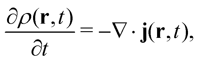 | (65) |
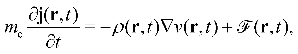 | (66) |
(r, t) is the force density arising from interactions between the particles. The calculation of the force density from the expectation value of the corresponding operator is a prohibitively difficult task: however, to the extent that we trust the basic tenets of time-dependent density and current DFT, we can assume that is a functional of the basic variables ρ and j. If an approximate form of this functional is adopted, then eqn (65) and (66) become a closed set of partial differential equations, akin to the equations of fluid mechanics, which can yield a huge amount of information about the evolution of the system without invoking the exact wave function. A particularly simple and appealing approximation to the force functional was proposed in ref. 571 and 572 for the linear response regime – that is, when the system is assumed to remain close to the ground state. The approximate force is then given by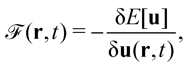 | (67) |
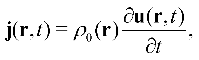 | (68) |
The elastic approximation is expected to work well for systems whose dynamics is dominated by collective modes, but not so well for independent-particle dynamics. There is much room for improvement, which makes this an exciting direction of research. Just to mention one possibility, the elastic approximation assumes that the force is instantaneously determined by the current: this leads to infinitely sharp excitation energies. We could go beyond the elastic approximation by introducing a physically motivated form of time retardation, which would immediately lead to more realistic spectra in extended systems.
4.2 What role will DFT play in multiscale and embedding methods?
 satisfies the following equality by construction:577
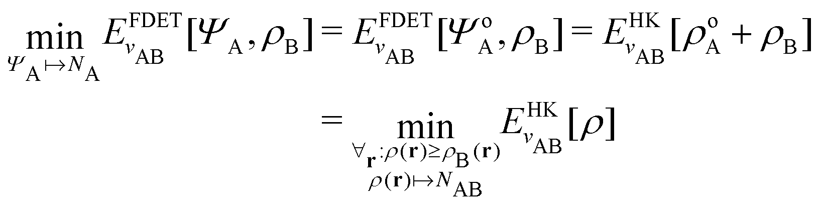 | (69) |
 . Recently, an expression for the total energy that (similarly to eqn (69)) is consistent with the Hohenberg–Kohn energy functional, was derived also for methods in which the correlation energy is obtained as a nonvariational correction to variationally obtained wave functions.578 For whatever form of the embedded wave function, including the one introduced by Wesolowski and Warshel,579 FDET represents a bottom-up approach to deal with the quantum embedding problem in multilevel/multiscale simulations.
The optimal total density is the sum of individual components ρB(r) and ρoA(r) considered as independent variables in the total energy expression. Such a choice of independent variables makes it possible to use the information about the environment of the embedded species obtained from any physical model capable of delivering ρB(r). Generating ρB(r) using a wave-function description of the environment is one of several possible choices. Other choices include ρB(r) obtained from continuum models of the environment,580 from X-ray diffraction data581 generated using a library of molecular electron densities,582 or from a simplified treatment of the electronic polarization.583 A particular version of FDET, where a noninteracting reference system is used for both ρA(r) and ρB(r) and where both densities are subject to optimization, is equivalent to Cortona's formulation of DFT.584
However, for all the reasons summarized above, when discussing orbital-free DFT, the KEDF potentials introduce errors one would like to avoid, since we do not yet have KEDFs that reliably work across the periodic table. Because of this, more than 10 years ago we proposed density-functional embedding theory (DFET),588 in which one eschews use of KEDF potentials and instead uses OEP theory to solve for an exact (within a given DFA) embedding potential that describes the interaction between the embedded region and its environment. (Note that DFET is fully generalizable to more than two subsystems but, since we are mostly interested in fairly localized phenomena, typically two subsystems of a cluster of atoms embedded in a periodic slab background is sufficient.) This embedding potential thus solved for is then “frozen”, with no approximation other than the choice of exchange–correlation functional used to perform the OEP calculation. Since exchange–correlation functionals in use today are much more accurate and transferable across the periodic table than KEDFs, the embedding potential thus derived is much more accurate as well. This frozen embedding potential then is added as a one-electron operator to the cluster Hamiltonian. Thereafter, one can exploit readily any quantum-chemistry method for conducting the ECW calculations.
See ref. 589 for a brief review and ref. 590 for a more in-depth review of DFET591 and its cousin, potential-functional embedding theory (PFET).592 The latter can deliver self-consistent embedding potentials for hybrid ECW/DFT systems,593–595 albeit at considerable cost. Frankly, we have yet to find cases in which such self-consistency was terribly important, although I imagine such cases will emerge. If one is careful to include sufficient numbers of atoms in the embedded region such that the embedding potential does not overlap the phenomenon of interest but instead is essentially a physical boundary condition, then the frozen exact embedding potential we derive from DFET works very well. Thus we have continued to use DFET/ECW theory rather than PFET – with considerable success – to study problems where conventional DFAs fail, such as for phenomena involving electron transfer596 and excited states involved in electrochemistry and photochemistry on metals; for a recent review on the latter, see ref. 597. You are welcome to utilize our codes that compute embedding potentials and the AO-integrals in a variety of formats (see ref. 598) to try these calculations for yourself. There you can also find codes for a generalization of DFET to nonlocal embedding potentials that can also describe covalently bonded systems, in what we refer to as density-matrix-functional embedding theory (DMFET), where the same idea of using OEP is applied to density matrices rather than densities.599,600
Recent benchmarks that we have conducted comparing electrochemical carbon dioxide reduction modelled by a conventional DFA versus DFET/ECW theory reveals critical insights for modellers: for qualitative conclusions regarding reactions that do not involve electron transfer, the DFA is acceptable.601 By contrast, for any step involving electron transfer, specifically proton-coupled electron transfer (which we find to be the most favourable pathway), the DFA fails on multiple fronts (specifically it yields results inconsistent with experiments) due to too facile electron transfer (as expected from self-interaction error and the lack of a derivative discontinuity) whereas DFET/ECW predictions agree with experiments and produces qualitatively different products than the DFA602 – a cautionary tale for DFT modellers of electrochemistry.
Finally, we recently extended DFET/ECW theory to ionic/covalent materials; nearly all our previous work was done on metals. Before solving for the embedding potential with OEP theory, we cap the dangling bonds that were created at fragment edges by initial covalent bond cleavage, while partitioning atoms into subsystems. The capping eliminates potential spin-polarization artefacts that unpaired electrons at fragment edges would produce. The DFET theory is modified to account for the density of the capping atoms while solving for the embedding potential.603 An interesting sustainable energy application using this new theory examined metal-to-ligand charge-transfer states in a Ru-bpy dye attached to a titania cluster, as a model for such excitations in a dye-sensitized solar cell. The ECW calculations were conducted at the embedded CASPT2 level, predicting both lifetimes of singlet excited states and the positioning of triplet excited states, in order to consider the competition between fluorescent and phosphorescent decay.604
Concerning the potential-functional embedding theory (PDFT), FDET expressions for the total energy and the embedding potential admit also the embedded wave function and the environment density obtained from PDFT. In such a case, the total energies and embedding potentials of PFET and FDET are expected to be the same, in the absence of additional assumptions and approximations. In their exact form, both approaches target the same solutions. The identity of the corresponding quantities, one given as an explicit functional of the environment density (FDET) and one not (self-consistent PFET), might lead to a better understanding of the relevant density functionals.
Concerning Cortona's formulation of DFT applied originally to atoms in solids, it is worthwhile to recall an intriguing observation regarding LDA made when it was used for intermolecular complexes in our exploratory works.605–607 For such complexes, LDA is known to be inadequate for approximating the exchange–correlation energy. However, when applied simultaneously for both the exchange–correlation and non-additive kinetic-energy functionals, LDA yields surprisingly good interaction energies. The reasons for this apparent compensation of errors remains an open question.
While this question may not belong to this section, and it may very well be that it is even ill-defined, our results obtained in ref. 608, especially the failure of the supermolecular TDDFT approach to produce accurate results for the same spectral shifts, made me wonder if practical implementations of TDDFT, which invoke a variety of approximations, satisfy the property of size intensivity of excitation energies (satisfied by properly developed methods based on equation-of-motion coupled-cluster theory). One might say that FDET and other embedding techniques are size intensive by design, which is yet another argument in their favour in applications involving excitation spectra in condensed phases.
We recently used the ab initio embedding scheme called the effective-fragment-potential approach609 combined with the aforementioned δ-CR-EOMCC(2,3) calculations, properly calibrated DFT and TDDFT methods to optimize geometries, and the DFT continuum solvation model based on the solute-electron-density approach610 to accurately model photochemistry of the strongest known super photobase abbreviated as FR0-SB in various alcohol solutions.611 This would not be possible without mixing DFT and TDDFT with embedding and ab initio approaches.
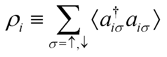 play the role of the density and the correlation embedding potential,616 which is used in the full-size system, is a collection of one-electron (“on-site” in lattice models615) energies vi. The latter are adjusted so that the corresponding embedded impurity orbitals have the same occupation as in the full-size system. Referring to a noninteracting Kohn–Sham (full-size) system in this context is appealing because it is a way to “exactify” the embedding procedure.
In regular DMET, the bath orbitals (which exchange electrons with the impurity orbitals) are constructed from the Schmidt decomposition of the approximate mean-field wave function (which is computed for the full system). The resulting reduced-in-size “impurity + bath” cluster is then treated in wave-function theory as a closed system.
Sekaran et al. have recently shown that this procedure is equivalent to a (much simpler) density matrix-functional Householder transformation when the density matrix is idempotent.615 They have also shown that, when the transformation is applied to a correlated density matrix, the cluster becomes an open subsystem. Therefore, if the full system is described at the noninteracting Kohn–Sham level (which is still exact density-wise), then the usual separation of the cluster from its environment is perfectly justified. The correlation potential then learns from the cluster (in which interactions are reintroduced, after applying the Householder transformation) through the density constraint.
Thus, we obtain a new type of density-functional approximation (with an implicit dependence on the density) where we can afford an accurate description of strong electron correlation. Obviously, in general, the cluster's environment (which is usually neglected) contributes to the total correlation energy. A formally exact density-functional embedding theory would in principle be obtained by deriving, in this context, a multireference version of Görling–Levy perturbation theory.133,449,450,615
This motivated the development of composite Kohn–Sham-DFT methods – for example, from the 3c-family B97-3c or r2SCAN-3c620,621 at the (meta)GGA level. The sought-after compromise between computational effort and accuracy is achieved here by applying tailored, medium-sized atom-centred AO basis sets on top of standard or slightly modified DFAs and adding appropriate atom pairwise potentials to account for dispersion and basis-set incompleteness. The recently proposed r2SCAN-3c method outperforms some hybrid-DFT/QZ approaches for reaction and conformational energies as well as for noncovalent interactions at a speed-up of two to three orders of magnitude.621
Fragment-based methods such as the explicit polarization (X-Pol) model can be designed as general QM/QM embedding approaches in which each fragment can be individually represented by any electronic-structure method, with the inclusion of the instantaneous environmental effects through Hartree, Pauli exchange, and dispersion potentials.626 Importantly, X-Pol and other fragment-based methods provide a framework for the development of next-generation quantum-mechanics force fields (QMFFs) for condensed-phase and biomolecular simulations.627 In a QMFF, QM effects such as polarization, charge transfer, and the change of the potential-energy surface itself due to dynamical fluctuations as well as chemical reactions are naturally included. These effects would be very difficult, if not impossible, to describe using the current MM force fields.
4.3 In what areas of application are improvements needed?
Nevertheless, the relationship between E[v,A] and F[ρ,jp] is sufficient to establish the Vignale–Rasolt formulation as a rigorous extension of DFT to systems in an external magnetic field. To obtain a convex formulation, however, the change of variables u = v + |A|2/2 is needed, imposing a formulation of the theory where the potential space can absorb the norm squared of the vector potential.629 Such a formulation of CDFT inherits the mathematical structure of standard DFT, only lacking the uniqueness provided by a Hohenberg–Kohn result.
The lack of a Hohenberg–Kohn theorem for CDFT has led to confusion in the literature and some (erroneous) claims questioning the validity of the Vignale–Rasolt formulation – see ref. 630 and 631 for a discussion of these points. Aside from these controversies, questions regarding the mathematical properties of F[ρ,jp] remained unclear, particularly regarding whether a formulation analogous to Lieb's treatment of DFT could be established for CDFT.
Such a Legendre–Fenchel formulation of CDFT was developed in ref. 631–633 but the equivalence of the Vignale–Rasolt constrained-search functional and the Lieb-type functional was only very recently established with the proof of the lower semicontinuity and expectation-valued nature of F[ρ,jp].634 The expectation-valuedness is important for the AC since it allows the energy to be partitioned (into exchange and correlation parts) in terms of the minimizing density matrix (or wave function) that satisfies the density constraint.
The Kohn–Sham formulation of CDFT was introduced already in 1987628,635 and recently several practical implementations of this approach for general molecular systems using London atomic orbitals for gauge-origin independence have appeared.636–638 As CDFT becomes a more widely applicable and practical tool for molecular simulations, several open questions remain both from a theoretical and a numerical point of view:
Representability. For CDFT, representability issues may be more acute.639,640 To what extent may ensemble approaches play a role in this context?
Current-dependent functionals. Approximate current-dependent exchange–correlation functionals Exc[ρ,jp] are still in an early stage of development although some approaches have been presented for extending existing DFAs.641–645 Those based on meta-GGA functionals have shown some promise in strong fields.39 However, improvements for low-field properties such as NMR shieldings, central to chemistry, are more modest.646 What is the optimal gauge-invariant parameterization of Exc[ρ,jp]? How may new functionals be developed and tested?
Alternative formulations of DFT in a magnetic field. CDFT is not the only way to extend DFT to systems in a magnetic field. The magnetic DFT (BDFT) formulation of Grayce and Harris requires functionals of the form E[v;B] and F[ρ;B], which simplifies numerical implementation and avoids an explicit functional dependence on jp, at the cost of losing some degree of universality.647,648 Could the simplifications outweigh the loss of universality in practical implementations? Another alternative would be to consider the coupling of internal magnetic fields with the external field via a Maxwell–Kohn–Sham approach, which does feature a Hohenberg–Kohn result for the total current density.649 Such an extension may be important in strong-field time-dependent light–matter interactions650 and leads to a more appealing functional dependence on the total current density, rather than only on its paramagnetic component. Finally, we mention linear-vector-potential DFT (LDFT), a simplified formulation of CDFT suitable for uniform magnetic fields.651
Given recent strides in better understanding the theoretical foundations of CDFT, and the construction of several practical implementations, addressing these challenges should lead to further progress and improvements in the accuracy of magnetic response properties with DFAs.
At least for molecular systems, pure functionals are not yet practically useful. Instead, the more pragmatic meta-GGA functionals are presently much better at capturing the response to magnetic fields. However, recent work has shown that the kinetic energy density employed in these meta-GGA functionals only builds in the correct gauge correction, but not any vorticity dependence.
One way forward is to employ a local tensor, akin to a stress-energy tensor, that encodes both the vorticity and a gauge-invariant kinetic energy in a natural way;653 see also the current dependent meta-GGA form in ref. 654. This tensor furthermore obeys strong N-representability conditions that enable discrimination of regions with one, two, three, and four-or-more Kohn–Sham orbitals. The isoorbital indicators that underlie many standard approximations discriminate rigorously only between one and two-or-more orbitals.
Fortunately, there are many indications that the “nonuniqueness” of the potential is harmless for Kohn–Sham applications because the wave function remains unique even when the potential is not. However, I do feel that all multivariable DFTs have another hidden problem – namely, to what extent can the intensive variables of the theory be varied arbitrarily and independently of each other? This problem may be particularly severe when there are global constraints enforced by symmetry – for example, the total angular momentum of a rotationally symmetric system. Or there may be inequalities whereby the maximum value of a density (say, the spin density) can never exceed some maximum value that is controlled by another density (say, the particle density). Such constraints affect the intensive variables but not their conjugate fields, which can always be varied independently. This is one of the main reasons (if not the only one) why the map from densities to potentials is generally not invertible.
4.4 What extensions are needed to get ground- and excited-state properties and observables in DFT?
 is the operator for the observable Q, then the density functional Q[ρ] is given by
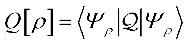 | (70) |
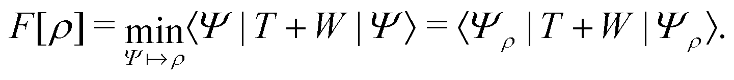 | (71) |
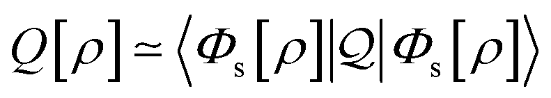 | (72) |
Since the definition of the density functional of a general observable is known, the development of an approximate or exact density functional Q[ρ] means trying to find an exact or approximate expression that does not depend on the unknown interacting state Ψρ, but which depends only on the density and also on quantities that can be obtained from a Kohn–Sham calculation (e.g., the Kohn–Sham state, orbitals, and eigenvalues) and which is more accurate than the obvious approximation in eqn (72). Recently, we managed to write down such a density functional for the magnetization density in DFT (not spin DFT) for open-shell systems in the absence of an external magnetic field.657
TDDFT has been overwhelmingly successful for a wide range of excited-state properties, but there are also spectacular failures. In the linear response regime, for example, it is now well understood that caution should exercised when standard DFAs are used to study states of double-excitation or charge-transfer character, and that these standard DFAs fail to yield excitonic spectra of semiconductors. However, such failures provide us with an opportunity to learn and improve our DFAs – much work remains to be done, but progress has been steady. It is also worth noting that the effort is well spent, given that TDDFT computations have a far smaller carbon footprint than alternative methods.
1. for extended systems, it allows a well-defined expression for the macroscopic polarization of the system in terms of the induced current–density in the bulk;668,669
2. it allows one to treat the response to transverse fields;670,671
3. instead of looking for frequency-dependent approximations to the exchange–correlation kernel that are nonlocal functionals of the density (as done in TDDFT), one can look for consistent frequency-dependent approximations that are local functionals of the current–density, such as the Vignale–Kohn (VK) functional.672
Recently, Berger proposed a functional in the context of TDCDFT that can describe excitons in 3D materials.673 Linear response of 2D materials by contrast remains a challenge in TD(C)DFT.674
This approach of DFT to molecular properties is not only interesting from a fundamental point of view; it can also show how far the present ideas for generating approximations can be taken – or help us understand why our current ideas work for the energy but not for a given property.
4.5 How can DFT further benefit from rigorous developments?
Several mathematical problems are still open and it would be nice to discuss here which of those could have an impact in DFT. I will only mention three problems which, in my opinion, deserve attention in the future.
The first is to better understand the Kohn–Sham potential. We have no rigorous proof that vs, which appears in eqn (8) and (32), for example, exists and, to my knowledge, no efficient numerical tool to construct an approximate one exists. Let me try to be a bit more precise.
Recall that a density ρ is (ensemble) v-representable when it arises from an N-electron (mixed) ground state with an external potential v. Let me emphasize that there are two notions of v-representability, for the interacting and noninteracting cases, respectively. The question is whether a v-representable density (for the interacting system) is v-representable by the noninteracting system. In other words, we need to study the set of densities that are simultaneously v-representable for the two cases. At the moment, nothing is known rigorously about this set, to my knowledge – in principle, it could even be empty! Of course, to properly discuss this problem, it is important to first fix a class of admissible potentials v that we wish to consider in DFT. This class should be large in order to increase the probability of being v-representable, but probably not too crazy either. Lieb considered all potentials belonging to L3/2(3) + L∞(3) because the energy is always bounded-below for such potentials.8 However, many physical cases do not appear in this class, such as the harmonic potential for instance. This is definitely a too small class.
One can understand v-representability in several other equivalent ways, all described by Lieb.8 My preference goes towards the Legendre–Frenchel point of view, which requires the use of mixed states and ensemble v-representability and was already discussed above in contributions (2.1.13) and (3.7.2). We know that the corresponding lowest total energy and the lowest kinetic energy for a given density ρ satisfy the duality principles8
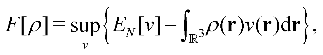 | (73) |
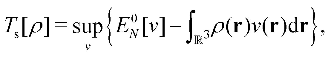 | (74) |
Another point of view has been mentioned above in contributions (2.2.2) and (3.7.2) and involves a kind of differentiability of F[ρ] and Ts[ρ]. Any potential solving a maximum principle such as in eqn (74) is, formally at least, a derivative of the corresponding functional.8 To be able to treat the difference F[ρ] − Ts[ρ], we thus need both to be differentiable at the same time. Although the notion of differentiability looks natural and intuitive, it is in fact not so easy. The reason is that the natural domain of F[ρ] is the set of densities with a finite von Weizäcker energy,8 which is not such a nice set.
Lieb proved that the two sets of v-representable densities are dense in the space L1(3) ∩ L3(3).8 The problem is that a dense set can, in principle, be extremely small – think of the rational numbers, which are dense but form a set of zero measure in the set of real numbers. Even worse, we need to look at the intersection of these two dense sets, which can be arbitrarily small or even empty. Very little is thus known mathematically about this problem.681
Let me now quickly mention the other two problems I had in mind. The second one is to improve existing exact constraints. For instance, I already mentioned the Lieb–Oxford bound,677 of which the best constant is believed to be that of the uniform electron gas.177,682,683 But at present, we have no idea on how to justify this rigorously.
Finally, I would like to mention that, unlike ground-state DFT, TDDFT is very poorly understood mathematically.684
![[scr I, script letter I]](https://www.rsc.org/images/entities/char_e143.gif) N.
N (namely, on the set of ensemble v-representable densities
N.
N (namely, on the set of ensemble v-representable densities ![[scr B, script letter B]](https://www.rsc.org/images/entities/char_e13f.gif) N) follows from the convexity and lower semicontinuity of the universal density functional F. It is a general result of convex analysis that a proper lower semicontinuous convex function (here F) is subdifferentiable on a dense subset (here N) of its effective domain (here N) and everywhere in the interior of its effective domain (here the empty set since N has no interior).
N) follows from the convexity and lower semicontinuity of the universal density functional F. It is a general result of convex analysis that a proper lower semicontinuous convex function (here F) is subdifferentiable on a dense subset (here N) of its effective domain (here N) and everywhere in the interior of its effective domain (here the empty set since N has no interior).
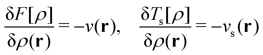 | (75) |
However, imagine that we change the ground-state energy in the manner
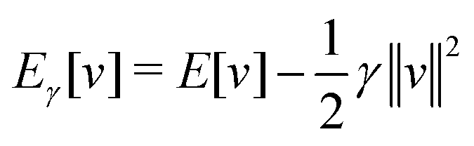
and likewise for (Ts)γ. Importantly, Fγ and (Ts)γ are both everywhere differentiable, meaning that the interacting and noninteracting Euler–Lagrange equations can now be solved simultaneously.99,686 In convex analysis, such a procedure is known as Moreau–Yosida regularization.687 Once the regularized energy Eγ[v] has been calculated, it is trivial to obtain E[v] and nothing is lost – that is, the Moreau–Yosida regularization of F has the curious property of being lossless with respect to the calculation of the ground-state energy E[v]. The only caveat is that ‖v‖ must be finite, which is only satisfied for Coulomb potentials by constraining the system to an arbitrarily large box.
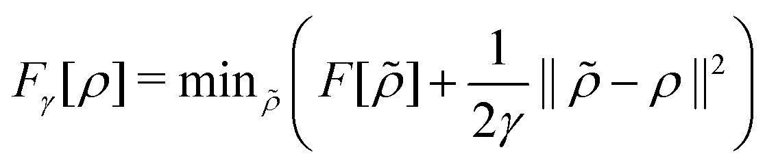
In the regularized setting, every density is both interacting and noninteracting representable – a rigorous exact Kohn–Sham theory is thereby established. However, such a density need not be a “physical” density.
The Moreau–Yosida regularization of DFT may also be of practical interest as a tool for guaranteeing and improving convergence of the Kohn–Sham iterations.99,688
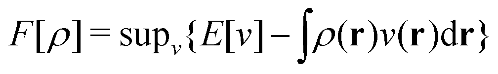 (see contribution (2.1.13)) attaining its maximum, such that ρ is representable by its maximizing potential. In analogy with the above discussion of the Moreau-Yosida procedure, a maximizing potential can here be guaranteed by a regularization of
 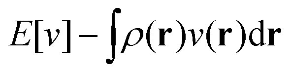 using fixed weight functions αi ∈ L∞. Such a scheme only makes use of partial information of the density constraint, i.e.,
  , for all i (for more details see ref. 689).
 | (76) |
Some open questions that remain on the rigorous side concern the next leading term in the ℏ → 0 expansion, whose form was conjectured in ref. 144. A first step in this direction has been recently taken.696 I do have the feeling that there is still a lot to learn from the connection with optimal transport and by further analysing this limit, which provides complementary information with respect to perturbation theory. Although it is a semiclassical limit, it may perhaps be corrected for exchange (spin) effects,697 and could be combined with Kohn–Sham DFT.408,698
A point in case is the Lieb–Oxford bound.677,695 Becke argued that any reasonable exchange functional globally satisfies the Lieb–Oxford bound for any real chemical or physical system, irrespective of whether the underlying energy density obeys or violates it locally.701 In other words, a local Lieb–Oxford bound seems to be a sufficient but not a necessary constraint in the design of functionals – the exact-exchange energy density, in particular, violates the local Lieb–Oxford bound in the tail of any finite system. A local enforcement of the Lieb–Oxford bound gives enhancement factors of some widely used semilocal exchange functionals (e.g., PBE234 and SCAN235 functionals) that are somewhat too low to describe finite systems adequately (in combination with an appropriate correlation functional), thus hampering thermochemical accuracy.
 , external forces, and internal kinetic and many-body stresses. The fixed-point technique is mathematically very difficult and the TDDFT proofs based on it are still not fully rigorous.98
It has recently been shown that TDDFT can be reformulated using  instead of ρ(r, t) as the basic variable, which has the advantage that the causal structure of the theory becomes more transparent.703 This result may provide a new way forward in the ongoing attempts to solidify the foundations of TDDFT.
4.6 How can DFT further benefit from numerical analysis and algorithmic developments?
Let us emphasize that the apparently simple case of a genuine, periodic crystal can be challenging also when the crystal is a metal. Recall that, for periodic crystals, using a supercell is mathematically equivalent to sampling the Brillouin zone with the regular k-point grid;713 the advantage of the latter approach is that it is far more efficient from a computational viewpoint. In most calculations, a relatively coarse k-point grid is used to further reduce the computational burden (say, 3 × 3 × 3 for insulators and 7 × 7 × 7 for metals). This approach is usually sufficient for insulators because the integrands are periodic, analytic, and weakly oscillating over the Brillouin zone for all relevant physical observables, but far from sufficient714 for metals with complicated Fermi surfaces. Smearing techniques715 at a fictitious positive temperature (possibly higher than the melting temperature of the metal) help to some extent,716 but do not fully solve the problem. It appears that many computational results on metals reported in the literature cannot be considered as converged with respect to k-point discretization.
Many groups have worked on the development of ![[scr O, script letter O]](https://www.rsc.org/images/entities/char_e52e.gif) (N) techniques, from the early nineties up to very recently. Nevertheless, robust (N) techniques for first-principles MD, where energies can be evaluated with a controlled error, are not yet available. Based on the experience acquired in the literature with (N) methods implemented using plane waves, wavelets, or other localized basis sets, it appears that methods with controllable accuracy might come from the development of real-space based techniques, which would also require the development of specific pseudopotentials for periodic DFT calculations.718
(N) techniques, from the early nineties up to very recently. Nevertheless, robust (N) techniques for first-principles MD, where energies can be evaluated with a controlled error, are not yet available. Based on the experience acquired in the literature with (N) methods implemented using plane waves, wavelets, or other localized basis sets, it appears that methods with controllable accuracy might come from the development of real-space based techniques, which would also require the development of specific pseudopotentials for periodic DFT calculations.718
Providing partial answers to these questions is the purpose of a field of applied mathematics called a posteriori error analysis. This field has reached its maturity in, for example, finite-element based computational mechanics, where most academic and commercial codes provide numerical results (e.g., the lift and drag of an aircraft) complemented by error bars. To understand what can or cannot be done in this direction for DFT, it is useful to decompose the overall error in several pieces:
1. the model error, coming from replacing the reference very accurate model (the N-body Schrödinger model or one of its relativistic counterparts) by a DFT approximation (LDA, PBE, B3LYP, etc.), possibly with pseudopotentials;
2. the discretization error due to the use of a finite basis set;
3. the algorithmic error due to finite convergence thresholds;
4. the finite-arithmetic error (computations are usually done in double precision);
5. execution error (negligible for current computers but an issue for future exascale719,720 and quantum computers).
It is already possible to estimate the discretization, algorithmic, and finite-arithmetic errors for linear Schrödinger equations discretized in plane-wave basis sets.721,722 The more recently developed error estimators are
1. guaranteed: mathematical theorems prove that the exact value indeed lies in the confidence interval;
2. accurate: the actual error is of the same order of magnitude as the error bar;
3. cheap to compute: evaluating the error bars requires only a moderate computational extra cost; and
4. systematically improvable: provide detailed information on how to increase the accuracy at the lowest cost.
Extending these techniques to the nonlinear Schrödinger and Kohn–Sham equations is work in progress.723 Such estimators would allow the computer program to choose adaptively, in a black-box manner, the best numerical parameters to reach a given numerical accuracy at the lowest computational cost (error balancing). Error balancing would be particularly useful for building large databases for ML, requiring hundreds of millions of single-point DFT calculations.724
Let us finally discuss the model error. For wave-function methods, it is in principle possible to estimate this component of the error by a careful mathematical analysis of the residual HNΨappN − ENΨappN, where HN is the N-electron Hamiltonian, and ΨappN and ENapp are the computed approximations to the ground-state wave function and energy; this is a topic of ongoing research. In the DFT setting, a promising approach is the use of (non-guaranteed) estimates based on a statistical analysis of the model error – see, for example, ref. 341–343 and 346. Whether nonstatistical, guaranteed, accurate, and cheap-to-compute model error estimators can be constructed using DFT is a completely open question.
4.7 What role will machine learning play in the future of DFAs and DFT?
 ground-state energy (and even everything)” may be a case where an AI model can capture the relationship better than a mathematical functional. However, at present, the flexibility of AI comes together with a lack of interpretability, and the missing knowledge of the domain of applicability is probably an even more severe problem for AI models than it is for DFAs. AI can only predict aspects that were included in the training. If this is considered sufficient, then AI is a numerically efficient approach, once the laborious training has been performed with appropriate care.
4.8 How should interpretive tools based on DFT evolve?
1. Is the use of a temperature-dependent version of conceptual DFT729 necessary to avoid the E(N) differentiability problem when considering temperatures typical for laboratory conditions in synthetic work (leaving high-temperature chemistry aside)?
2. Can the pros and cons of going from the canonical ensemble, with the associated E[N, v] functional, to the grand canonical ensemble, with a state function Ω[μ, v] that allows fluctuations in the number of electrons,730 be clarified for the practising chemist? See also contribution (2.4.1).
3. Can one expect that the perturbation series of E[N, v] of a given reactant upon interaction with a perturbing reaction partner (the second reactant) converges properly in most cases?
4. Can the proper use of the principles mentioned in contribution (3.9.1) be supported by delineating their domain of applicability – that is, by formulating the conditions under which a meaningful application of the different principles is possible?
5. Can potential pitfalls in using conceptual DFT when going from kinetic (reactivity) to thermodynamic (stability) reasoning be identified?
On the other hand, the theory is in need of extensions – for example:
1. the inclusion of new variables in the E[N, v] functional such as electric and magnetic fields, mechanical forces, pressure to cope with the increasing variety of reaction conditions encountered in present-day chemistry;731,732
2. a proper and possibly elegant inclusion of spin733 to extend the theory to transition metals, of crucial importance in catalysis, and to radical reactions;
3. a generally applicable extension to excited-state reactivity482,734,735 to deepen the insight into photochemical phenomena and, in the same vein, an extension to time-dependent conceptual DFT;736
4. a deeper connection between conceptual DFT and information theory and its density functionals193,737 and with the reaction-force ansatz when considering reaction mechanisms.738
Recognizing that the ultimate goal of conceptual DFT is prediction, it was realized that the one reactant approach on the basis of the above mentioned E[N, v] expansion should be scrutinized to identify what terms in the expansion of E[N, v] are most likely to be efficient for a given problem, thereby challenging chemical intuition. Characteristics of the second reactant most probably should be explicitly introduced at various levels of refinement for quantifying the ΔN and Δv perturbations.475
Recently, a general approach was introduced for treating spin-coupling interactions of open-shell molecules by MSDFT.458 The TDF energies that determine spin coupling are obtained by enforcing the multiplet degeneracy of the S + 1 state in the MS = S manifold. Spin-adapted configuration states were used as the active space in MSDFT calculations of core excitations of open-shell molecules.
5 Communicating and sharing our results
5.1 How should the DFT community organize and share information?
One such DFT-specific aspect has been pointed out by Loos in his contribution (5.1.1). But as usual there is a hitch. First, just because a DFA (or KEDF) is implemented for some kind of Gaussians, this doesn’t mean that it will work for a plane-wave PAW code. (It may not even work for another kind of Gaussians without some fiddling.) Secondly, there are mis-implementations. (The B3LYP DFA itself is a kind of mis-implementation and there are the notorious VWN versions.) Postdocs in my group have found several mis-implementations in popular codes and one of our finite-temperature DFAs was mis-implemented in libxc. Especially for intricate DFAs (and KEDFs), it seems healthier to have several independent implementations.
Another step would be for presentation of a new DFA to include an explicit, unambiguous statement near the outset of whether it was intended for only a certain class of molecules or only for molecules but not condensed phases, etc. and on what class of systems it had been tested.
Libraries and modules such as these not only provide high performance, but also improved reproducibility and standardization, both of which are becoming more vital as the complexity of our models advances. To that end, emerging standards and tools for sharing computational results will similarly grow in importance. In the materials-science domain, for example, this has long been underway with community-driven resources such as the Materials Project758 as a paradigm, although the standardization of the content of materials databases is still under development within that community. In the computational-chemistry domain, new tools such as the Quantum Chemistry Schema (QCSchema) and Quantum Chemistry Archive (QCArchive)759 (an open, public-facing database of computational results) developed by the Molecular Sciences Software Institute (MolSSI)760,761 would allow much greater interoperability between codes by facilitating standards for data sharing. In addition, the Simulation Environment for Atomistic and Molecular Modeling (SEAMM),762 also under development by the MolSSI, provides a lightweight, Python-based plug-in environment for complex, shareable workflows, which will permit sophisticated computations involving multiple community code components in a fully reproducible and publishable manner. The broader the adoption of standards and tools such as these, the faster our community will be equipped to handle more complex and important scientific challenges.
5.2 How and what should we publish?
Identifying something as “broken” and/or “unsustainable” as in contribution (5.2.2) could be the first step towards repairing it, but I am not optimistic. I am reminded of the alleged response of a local in rural Ireland: “If I wanted to get to Dublin, I wouldn’t start here.” Ever-increasing pressure to obtain external funding will both hamper risk-taking and increase focus on “fashionable” topics.
5.3 What format should workshops and conferences take in the future?
We should work out new formats that do not force us to choose between taking a plane and having coffee with colleagues, or just sitting in front of a screen. We could work out, for example, a delocalized physical conference, where smaller hubs are connected by internet and people can travel to the nearest hub. Such a format would necessitate new forms of discussion but, if we are not too conservative, we can certainly come up with solutions. Besides, online tools also allow us to make material available in advance, such that newcomers in the field can be better prepared and profit more.
5.4 How can we best teach and communicate DFT?
The Hohenberg–Kohn theorem5 is ubiquitous, but little used in practice. Its proper place today is in review articles and textbooks, and we should focus on the constrained-search approach6 and the formulation of DFT in terms of Legendre transforms.8 Kutzelnigg's “beginner's” guide to the latter is accessible to most in the DFT field.771
As noted in contribution (2.1.13), “the power of DFT derives from Kohn–Sham theory,” but the successes of Kohn–Sham theory are linked closely to the ability of local density approximations to the exchange–correlation energy Exc to give useful results in most cases. Kohn noted: “I believe that formal DFT would have been of very little interest if there had not been a simple and very practical approximation for Exc, the LDA, which has yielded surprisingly accurate results.”772
Kohn and Sham proposed using an LDA for Exc that is exact in two limits (slowly varying densities and high densities).65 These are far from the density distributions found in atoms, molecules, and condensed matter. Kohn and Sham, and many others, were therefore convinced that LDAs would not describe chemical bonding well. Nevertheless, they gave “reasonable” answers in early tests of energy differences (including small molecules120,469,773 and jellium half-spaces100,119) and remain the basis of many approximations for Exc. The initial successes of LDA were so surprising that they motivated work to understand why it could provide useful energy differences for systems with densities far from the regions of obvious validity. This work led to “adiabatic coupling” and studies of the exchange and correlation holes, their spherical averages and related sum rules,100,119,120 which have been of lasting value in DFT studies. This surprisingly satisfactory description of reality often provided by LDAs was essential to the ultimate success of DFT.
When teaching DFT to beginners, we face similar choices as in other fields of physics (e.g., quantum mechanics, electrodynamics): we can follow the historical path in which the field was established, or we can start with the most fundamental theorems and then build up the formalism, or we can introduce the subject through examples, case studies, and hands-on applications. In our experience, students tend to learn DFT better when the latter approach is taken; if we start with the theorems or with many-body theory, students often fail to see the connection to the “real world”. Thus, as a community, we should make an effort to make DFT more accessible and inclusive, and to do this it will be helpful to develop (and share) simple numerical examples and hands-on exercises.
1. To understand the theory behind DFT, you need to have a good understanding of many-electron wave functions and reduced density matrices, especially in real space, which they often lack.
2. Most pedagogical material focuses on DFT without spin densities, while in applications the latter are used.
3. Modern exchange–correlation functionals are very complicated and look obscure to them.
4. The language is often ambiguous – for example, in the literature and in conferences the term “local” is sometimes used to indicate a multiplicative potential (the local Kohn–Sham potential, as opposed to the nonlocal Hartree–Fock potential) and sometimes to indicate a local dependence on the density.
5. The role of symmetry breaking is very important and often neglected in pedagogical material.
Finally, I believe it would be useful to teach LDA in a more modern way, by including the recent works on the large – N limit of neutral atoms, which show in which sense LDA is a universal limit for Coulombically bound systems and how gradient expansions arise; see, for example, ref. 179 for a recent review.
• We know in principle how to calculate observables in terms of many-body wave functions, but we cannot do it in practice in most cases. The choice of DFT, instead, is to express ground-state observables as functionals of the ground-state density. The density is an object that is more compact (depending on fewer variables) than the many-body wave function;
• We could also express observables as functionals of other quantities that are more compact than many-body wave functions – DFT uses the ground-state density, but we could also choose density matrices, for example, as a good descriptor;
• As a rule of thumb, the more compact we make the descriptor, the fewer observables can be calculated as explicit functionals. We can therefore discuss when and why the density is a convenient choice – for example, when the Hartree energy is important;
• The idea to use an auxiliary system to determine one or more, but perhaps not all, observables exactly should be exposed clearly;
• In many-body physics, we know from the very start that approximations will be needed. It is then crucial to discuss why DFT is a good starting point for approximations;
• We should also discuss the choice of strategies for developing approximations, rather than the technical details. One example in DFT is to calculate the kinetic energy from a noninteracting system with the same density as the interacting one. Another example is to use the intuitive concept of nearsightedness.184,185
These are very general ideas that can be found – maybe under different names – also in contexts other than DFT, but they have all been important for the success of DFT.
Conflicts of interest
There are no conflicts to declare.Appendices
A Acronyms
| AC | Adiabatic connection |
| ACFD | Adiabatic-connection fluctuation-dissipation |
| ADFT | Auxiliary DFT |
| AI | Artificial intelligence |
| AIMD | Ab initio MD |
| AM1 | Austin Model 1 |
| BBGKY | Bogoliubov–Born–Green–Kirkwood–Yvon |
| BCB | Bottom of the conduction band |
| BDFT | Magnetic DFT |
| BLW | Block-localized wave function |
| BOMD | Born–Oppenheimer molecular dynamics |
| BSE | Bethe–Salpeter equation |
| CASPiDFT/CASΠDFT | CAS pair-density functional theory |
| CASSCF | Complete-active-space SCF |
| CASPT2 | Complete-active-space PT2 |
| CCSD | Coupled-cluster singles–doubles |
| CCSD(T) | CCSD with perturbative triples |
| CDFT | Current DFT |
| CI | Configuration interaction |
| DC | Dirac–Coulomb |
| DD | Density driven |
| DEKS | Direct-energy Kohn–Sham |
| DF | Density functional |
| DFA | Density-functional approximation |
| DFET | Density-functional embedding theory |
| DFT | Density-functional theory |
| DFTB | Density-functional tight binding |
| DFT+U | DFT with the Hubbard U correction |
| DK | Douglas–Kroll |
| DMET | Density-matrix embedding theory |
| DMFT | Density-matrix functional theory |
| DMRG | Density-matrix renormalization group |
| dRPA | Direct RPA |
| EA | Electron affinity |
| ECW | Embedded correlated wave function |
| EDA | Energy decomposition analysis |
| EDFT | Ensemble DFT |
| EFG | Electric field gradient |
| ELS | Extended Löwdin–Shull |
| ELS + | Augmented ELS |
| EXX-OEP | Exact exchange – optimized effective potential |
| FCI | Full CI |
| FDET | Frozen-density embedding theory |
| FPMD | First-principles molecular dynamics |
| GASSCF | Generalized-active-space SCF |
| GGA | Generalized gradient approximation |
| GKS | Generalized Kohn–Sham |
| GL | Görling–Levy |
| GL2 | Second-order GL |
| GMTKN55 | General main-group thermochemistry, kinetics, and non-covalent interactions dataset |
| GW | Green's function G and screened Coulomb interaction W |
| GOEP | Generalized OEP |
| GOK | Gross–Oliveira–Kohn |
| HEG | Homogeneous electron gas |
| HF | Hartree–Fock |
| HK | Hohenberg–Kohn |
| HOMO | Highest occupied MO |
| Hxc | Hartree–exchange–correlation |
| IP | Ionization potential |
| i-DFT | DFT for steady-state transport |
| KE | Kinetic energy |
| KEDF | Kinetic-energy density functional |
| KS | Kohn–Sham |
| LFDFT | Ligand-field DFT |
| LD | Local density |
| LDA | Local density approximation |
| LH | Local hybrid |
| LOB | Lieb–Oxford bound |
| LR/lr | Long range |
| lrMCSCF–srDFT | Long-range MCSCF with short-range DFT |
| lrWFT–srDFT | Long-range WFT with short-range DFT |
| LUMO | Lowest occupied MO |
| MAE | Mean absolute error |
| MC | Multiconfigurational |
| MBPT | Many-body perturbation theory |
| MC-DFT | Multiconfiguration DFT |
| MC-NCFT | Multiconfiguration nonclassical functional theory |
| MC-PDFT | Multiconfiguration pair-density functional theory |
| MCSCF | Multiconfigurational SCF |
| MC-srDFT | MCSCF theory with short-range DFT |
| MD | Molecular dynamics |
| MD/MC | Molecular dynamics/Monte Carlo |
| MGCDB84 | Main-group chemistry database with 84 data sets |
| ML | Machine learning |
| MLP | Machine-learned potential |
| MM | Molecular mechanics |
| MMRDFTP | Mild-mannered respectable DFT practitioner |
| MNDO | Modified neglect of diatomic overlap |
| MO | Molecular orbital |
| MP4 | 4th-order Møller–Plesset |
| MSDFT | Multistate DFT |
| MSSCF | Multistate SCF |
| NEVPT2 | N-Electron valence state PT2 |
| NOSI | Nonorthogonal state interaction |
| NTO | Natural transition orbital |
| OEP | Optimized effective potential |
| OO | Orbital optimization |
| OT | Optimal transport |
| PAW | Projected augmented wave |
| PD | Pair density |
| PFET | Potential-functional embedding theory |
| PFT | Potential-functional theory |
| PM6 | Parameterization Method 6 |
| PPLB | Perdew–Parr–Levy–Balduz |
| PT2 | Second-order perturbation theory |
| PZ | Perdew–Zunger |
| QCT | Quantum-chemical topology |
| QE-DFT | Quasi-energy DFT |
| QED | Quantum electrodynamics |
| QM | Quantum mechanics/mechanical |
| QMC | Quantum Monte Carlo |
| QMFF | Quantum-mechanical force field |
| QM/MM | Quantum-mechanics/molecular-mechanics |
| QM/QM | Quantum-mechanics/quantum-mechanics |
| QTAIM | Quantum theory of atoms in molecules |
| QZ | Quadruple zeta |
| RASSCF | Restricted-active-space SCF |
| RDF | Relativistic DF |
| RDM | Reduced density matrix |
| RHEG | Relativistic HEG |
| RPA | Random-phase approximation |
| RS | Range separation |
| SA-CASSCF | State-averaged CASSCF |
| SAOP | Statistical averaging of orbital potentials |
| SCE | Strictly-correlated electrons |
| SCF | Self-consistent field |
| SF-TDDFT | Spin-flip TDDFT |
| SIC | Self-interaction correction |
| SIE | Self-interaction error |
| SR/sr | Short range |
| srDFT | Short-range DFT |
| SSE | Sham–Schlüter equation |
| SU(n) | Special unitary group of degree n |
| TAO-DFT | Thermally-assisted-occupied DFT |
| TB | Tight binding |
| TDCDFT | Time-dependent CDFT |
| TDDFT | Time-dependent DFT |
| TDDMFT | Time-dependent DMFT |
| TDF | Transition-density functional |
| TRIM | Trust-region image minimization |
| UEG | Uniform electron gas |
| vdW | van der Waals |
| WF | Wave function |
| WFT | Wave-function theory |
| XC | Exchange–correlation |
| X-Pol | Explicit polarization |
| X2C | Exact two-component |
| Xα | X-alpha method |
| ZDO | Zero differential overlap |
| ΔSCF | Delta-SCF |
| 1RDM | First-order reduced density matrix |
| 2RDM | Second-order reduced density matrix |
B Mathematical symbols
| A | Electron affinity |
| N | Set of ensemble v-representable densities |
| E | Total electronic energy |
| E H | Hartree density functional |
| E xc | Exchange–correlation density functional |
| E Hxc | E H + Exc |
| F | Universal density functional |
| f | Fukui function |
| H | Hamiltonian |
| I | Ionization potential |
| N | Set of N-representable densities |
| j μ | Four-current-density |
| j | Total current-density |
| j p | Paramagnetic current-density |
| L | Angular momentum |
|
L
p
(3) | Set of Lebesgue p-integrable functions on 3 |
| m | Magnetization density |
| m e | Electron mass |
| N | Number of electrons |
| R | Nuclear positions |
| r | Electron positions |
| s | Local softness |
| S 2 | Total spin squared |
| S | Chemical softness |
| t | Time |
| V |
|
| v | External potential |
| W |
|
| w | Potential of interaction between electrons |
| v s | Kohn–Sham potential |
| v xc | Exchange–correlation potential |
| T | Kinetic energy |
| T s | Kinetic energy of the Kohn–Sham noninteracting system |
| W | Two-particle interaction |
| Z | Nuclear charges |
| γ | First-order reduced density matrix |
| Γ | Two-particle reduced density matrix |
| λ | Coupling coefficient in adiabatic connection |
| μ | Chemical potential |
| ε | Orbital energy |
| ζ | Spin polarization |
| Φ | Slater determinant |
| ϕ | Orbital |
| Π | Pair density |
| ρ | Density |
| ρ Ψ |
ρ given by Ψ |
| σ | Spin index |
| ξ | Ensemble weight |
| Ψ | N-Electron wave function |
| η | Chemical hardness |
| χ | Linear response function |
| ω | Electrophilicity |
Acknowledgements
The authors are indebted to Steven Berry, Durham University, for preparation of the cover art graphics associated with this paper. AK acknowledges support from the U.S. National Science Foundation (NSF) through Grant No. CHE-2154482. AL acknowledges support from the Norwegian Research Council through Grant No. 287906 (CCerror) and 262695 (CoE Hylleraas Center for Quantum Molecular Sciences). AMK acknowledges support from the Mexican Consejo Nacional de Ciencia y Tecnología through Grant No. A1-S-11929. AMT acknowledges financial support from the European Research Council under H2020/ERC Consolidator Grant topDFT (Grant No. 772259). CAU is supported by DOE grant No. DE-SC0019109 and NSF grants No. DMR-1810922 and DMR-2149082. CD acknowledges funding by the German Research Foundation (DFG) through projects 460197019, 424709454, and 182087777 as well as by the European Union's Horizon 2020 research and innovation program under the grant agreement No. 951786 (NOMAD CoE). EAC acknowledges financial support from the Advanced Scientific Computing Research Program funded by the U.S. Department of Energy, Office of Science, Basic Energy Sciences, under Award No. DE-AC02-05CH11231. EC acknowledges support from the European Research Council (ERC) under H2020/ERC Grant EMC2 810367. EF thanks LabEx CSC (grant number: ANR-10-LABX-0026-CSC) and ANR (CoLab project, grant number: ANR-19-CE07-0024-02) for funding. ERJ thanks the Natural Sciences and Engineering Research Council of Canada (NSERC) for financial support. FDP and PG want to acknowledge the Vrije Universiteit Brussel for the support through a Strategic Research Program (SRP). GG acknowledges DOE/BES support through the Computational Materials Science Center MICCoM. HCh thanks gratefully C. Morell for his continuous support and for thorough discussions. JG acknowledges support from the U.S. National Institutes of Health under grant no. GM046736. JPP acknowledges support from the U.S. National Science Foundation under grant no. DMR-1939528 and from the U.S. Department of Energy under grant no. DE-SC0018331. LK is supported by the Helen and Martin Kimmel Award for Innovative Investigation and the Aryeh and Mintzi Katzman Professorial Chair. ML acknowledges support from the European Research Council (ERC) under H2020/ERC Grant MDFT 725528. MLe acknowledges support from the Julian Schwinger Foundation. MS acknowledges funding from the European Unions Horizon 2020 Research and Innovation Programme (No. 951786, the NOMAD Center of Excellence) and from the ERC Advanced Grant TEC1P (No. 740233). NG acknowledges financial support from The Leverhulme Trust, through a Research Project (Grant No. RPG-2016-005). PFL thanks the European Research Council (ERC) under the European Union's Horizon 2020 research and innovation programme (Grant agreement No. 863481) for financial support. PKC acknowledges DST, New Delhi, India for the J. C. Bose National Fellowship, grant number SR/S2/JCB-09/2009. PPi acknowledges support from the Chemical Sciences, Geosciences and Biosciences Division, Office of Basic Energy Sciences, Office of Science, U.S. Department of Energy under award no. DE-FG02-01ER15228. SBT is supported by U.S. DOE grant DE-SC0002139 and NSF grant DMR-1912618. TDC was supported by the Molecular Sciences Software Institute under U.S. National Science Foundation grants ACI-1547580 and CHE-2136142. TG acknowledges support from the Australian Research Council (grant no. DP200100033). TH acknowledges support from the Research Council of Norway for the CoE Hylleraas Centre for Molecular Sciences (Grant No. 262695). XX acknowledges support from the National Natural Science Foundation of China (Grant No. 21688102).Notes and references
- Overleaf, an open-source online real-time collaborative LaTeX editor, https://www.overleaf.com.
- F. Zahariev and M. Levy, Phys. Rev. A, 2019, 100, 062507 CrossRef CAS.
- E. Fermi, Z. Phys., 1928, 48, 73–79 CrossRef CAS.
- T. Kato, Commun. Pure Appl. Math., 1957, 10, 151–177 CrossRef.
- P. Hohenberg and W. Kohn, Phys. Rev., 1964, 136, B864–B871 CrossRef.
- M. Levy, Proc. Natl. Acad. Sci. U. S. A., 1979, 76, 6062–6065 CrossRef CAS PubMed.
- M. Levy, Phys. Rev. A: At., Mol., Opt. Phys., 1982, 26, 1200–1208 CrossRef CAS.
- E. H. Lieb, Int. J. Quantum Chem., 1983, 24, 243–277 CrossRef CAS.
- N. Schuch and F. Verstraete, Nat. Phys., 2009, 5, 732–735 Search PubMed.
- J. P. Perdew and A. Zunger, Phys. Rev. B: Condens. Matter Mater. Phys., 1981, 23, 5048–5079 CrossRef CAS.
- A. Savin, Theoretical and Computational Chemistry, Elsevier, 1996, pp. 327–357 Search PubMed.
- Y. Zhang and W. Yang, J. Chem. Phys., 1998, 109, 2604–2608 CrossRef CAS.
- A. D. Becke, J. Chem. Phys., 2005, 122, 064101 CrossRef PubMed.
- P. Mori-Sánchez, A. J. Cohen and W. Yang, J. Chem. Phys., 2006, 124, 091102 CrossRef.
- P. Mori-Sánchez, A. J. Cohen and W. Yang, J. Chem. Phys., 2006, 125, 201102 CrossRef PubMed.
- P. Mori-Sánchez, A. J. Cohen and W. T. Yang, Phys. Rev. Lett., 2008, 100, 146401 CrossRef PubMed.
- A. J. Cohen, P. Mori-Sánchez and W. Yang, Science, 2008, 321, 792–794 CrossRef CAS PubMed.
- J. P. Perdew, R. G. Parr, M. Levy and J. L. Balduz, Phys. Rev. Lett., 1982, 49, 1691–1694 CrossRef CAS.
- Y. Zhang and W. Yang, Theor. Chem. Acc., 2000, 103, 346–348 Search PubMed.
- W. Yang, Y. Zhang and P. W. Ayers, Phys. Rev. Lett., 2000, 84, 5172–5175 CrossRef CAS PubMed.
- A. J. Cohen, P. Mori-Sánchez and W. Yang, Phys. Rev. B: Condens. Matter Mater. Phys., 2008, 77, 115123 CrossRef.
- X. Zheng, A. J. Cohen, P. Mori-Sánchez, X. Hu and W. Yang, Phys. Rev. Lett., 2011, 107, 026403 CrossRef PubMed.
- C. Li, X. Zheng, N. Q. Su and W. Yang, Natl. Sci. Rev., 2018, 5, 203–215 CrossRef CAS.
- N. Q. Su, A. Mahler and W. Yang, J. Phys. Chem. Lett., 2020, 11, 1528–1535 CrossRef CAS PubMed.
- Y. Mei, Z. Chen and W. Yang, J. Phys. Chem. Lett., 2020, 11, 10269–10277 CrossRef CAS PubMed.
- A. J. Cohen, P. Mori-Sánchez and W. Yang, J. Chem. Phys., 2008, 129, 121104 CrossRef PubMed.
- P. Mori-Sánchez, A. J. Cohen and W. Yang, Phys. Rev. Lett., 2009, 102, 066403 CrossRef PubMed.
- N. Q. Su, C. Li and W. Yang, Proc. Natl. Acad. Sci. U. S. A., 2018, 115, 9678–9683 CrossRef CAS PubMed.
- P.-O. Löwdin, Int. J. Quantum Chem., 1985, 28, 19–37 CrossRef.
- W. Yang, P. W. Ayers and Q. Wu, Phys. Rev. Lett., 2004, 92, 146404 CrossRef PubMed.
- R. F. Nalewajski and R. G. Parr, J. Chem. Phys., 1982, 77, 399–407 CrossRef CAS.
- T. Helgaker and A. M. Teale, The physics and mathematics of Elliott Lieb, European Mathematical Society Press, London, 2022, vol. I, pp. 527–559 Search PubMed.
- M. Lewin, E. H. Lieb and R. Seiringer, 2020, arXiv e-prints, arXiv:1912.10424.
- P. E. Lammert, Phys. Rev. A: At., Mol., Opt. Phys., 2010, 82, 012109 CrossRef.
- L. Garrigue, Math. Phys. Anal. Geom., 2018, 21, 27 CrossRef.
- K. Capelle and G. Vignale, Phys. Rev. B: Condens. Matter Mater. Phys., 2002, 65, 113106 CrossRef.
- A. Laestadius and E. I. Tellgren, Phys. Rev. A, 2018, 97, 022514 CrossRef CAS.
- A. E. Clark, H. Adams, R. Hernandez, A. I. Krylov, A. M. N. Niklasson, S. Sarupria, Y. Wang, S. M. Wild and Q. Yang, ACS Cent. Sci., 2021, 7(8), 1271–1287 CrossRef CAS PubMed.
- J. W. Furness, J. Verbeke, E. I. Tellgren, S. Stopkowicz, U. Ekström, T. Helgaker and A. M. Teale, J. Chem. Theory Comput., 2015, 11, 4169–4181 CrossRef CAS PubMed.
- A. Görling, J. Chem. Phys., 2005, 123, 062203 CrossRef PubMed.
- R. T. Sharp and G. K. Horton, Phys. Rev., 1953, 90, 317 CrossRef.
- J. D. Talman and W. F. Shadwick, Phys. Rev. A: At., Mol., Opt. Phys., 1976, 14, 36–40 CrossRef CAS.
- A. Görling, Phys. Rev. Lett., 1999, 83, 5459–5462 CrossRef.
- S. Ivanov, S. Hirata and R. J. Bartlett, Phys. Rev. Lett., 1999, 83, 5455–5458 CrossRef CAS.
- S. Kümmel and L. Kronik, Rev. Mod. Phys., 2008, 80, 3–60 CrossRef.
- E. Trushin and A. Görling, J. Chem. Phys., 2021, 155, 054109 CrossRef CAS PubMed.
- R. G. Parr and W. Yang, Density Functional Theory of Atoms and Molecules, Oxford University Press, Oxford, 1989 Search PubMed.
- N. H. March and B. M. Deb, The single-particle density in physics and chemistry, Academic Press, London, 1987 Search PubMed.
- Chemical Reactivity Theory: A Density Functional View, ed. P. K. Chattaraj, CRC Press, Taylor & Francis Group, Florida, 2009 Search PubMed.
- N. D. Mermin, Phys. Rev., 1965, 137, A1441–A1443 CrossRef.
- V. V. Karasiev, T. Sjostrom, J. Dufty and S. B. Trickey, Phys. Rev. Lett., 2014, 112, 076403 CrossRef PubMed.
- T. Sjostrom and J. Daligault, Phys. Rev. Lett., 2014, 113, 155006 CrossRef PubMed.
- V. Karasiev, T. Sjostrom, D. Chakraborty, J. W. Dufty, F. E. Harris, K. Runge and S. B. Trickey, Frontiers and Challenges in Warm Dense Matter, Springer, 2014, pp. 61–85 Search PubMed.
- V. V. Karasiev, J. W. Dufty and S. B. Trickey, Phys. Rev. Lett., 2018, 120, 076401 CrossRef CAS PubMed.
- J. C. Smith, F. Sagredo and K. Burke, Frontiers of Quantum Chemistry, Springer, 2018, pp. 249–271 Search PubMed.
- V. V. Karasiev, S. B. Trickey and J. W. Dufty, Phys. Rev. B, 2019, 99, 195134 CrossRef CAS.
- A. K. Rajagopal and J. Callaway, Phys. Rev. B: Solid State, 1973, 7, 1912–1919 CrossRef CAS.
- E. Engel, Relativistic Electronic Structure Theory: Part 2. Applications, Elsevier, Amsterdam, 2004, pp. 523–621 Search PubMed.
- A. H. MacDonald and S. H. Vosko, J. Phys. C: Solid State Phys., 1979, 12, 2977–2990 CrossRef CAS.
- M. V. Ramana and A. K. Rajagopal, J. Phys. C: Solid State Phys., 1981, 14, 4291–4302 CrossRef.
- N. N. Bogoliubov, Problems of Dynamical Theory in Statistical Physics (in Russian) [Studies in Statistical Mechanics, edited by J. de Boer and G. E. Uhlenbeck, North-Holland, Amsterdam, 1961, vol. 1)], Gostekhisdat, Moscow, 1946 Search PubMed.
- E. R. Davidson, Reduced Density Matrices in Quantum Chemistry, Academic Press, London, 1976 Search PubMed.
- K. Pernal, O. Gritsenko and E. J. Baerends, Phys. Rev. A: At., Mol., Opt. Phys., 2007, 75, 012506 CrossRef.
- R. Van Meer, O. Gritsenko and J.-D. Chai, Phys. Rev. A, 2020, 102, 032815 CrossRef CAS.
- W. Kohn and L. J. Sham, Phys. Rev., 1965, 140, A1133–A1138 CrossRef.
- U. von Barth and L. Hedin, J. Phys. C: Solid State Phys., 1972, 5, 1629–1642 CrossRef CAS.
- A. Seidl, A. Görling, P. Vogl, J. A. Majewski and M. Levy, Phys. Rev. B: Condens. Matter Mater. Phys., 1996, 53, 3764–3774 CrossRef CAS PubMed.
- R. Garrick, A. Natan, T. Gould and L. Kronik, Phys. Rev. X, 2020, 10, 021040 CAS.
- E. J. Baerends and O. V. Gritsenko, J. Phys. Chem. A, 1997, 101, 5383–5403 CrossRef CAS.
- D. P. Chong, O. V. Gritsenko and E. J. Baerends, J. Chem. Phys., 2002, 116, 1760–1772 CrossRef CAS.
- O. V. Gritsenko, B. Braida and E. J. Baerends, J. Chem. Phys., 2003, 119, 1937–1950 CrossRef CAS.
- A. Savin, C. J. Umrigar and X. Gonze, Chem. Phys. Lett., 1998, 288, 391–395 CrossRef CAS.
- R. van Meer, O. V. Gritsenko and E. J. Baerends, J. Chem. Theory Comput., 2014, 10, 4432–4441 CrossRef CAS PubMed.
- A. I. Krylov, J. Chem. Phys., 2020, 153, 080901 CrossRef CAS PubMed.
- J. V. Ortiz, J. Chem. Phys., 2020, 153, 070902 CrossRef CAS PubMed.
- U. Salzner and R. Baer, J. Chem. Phys., 2009, 131, 231101 CrossRef PubMed.
- R. Baer, E. Livshits and U. Salzner, Annu. Rev. Phys. Chem., 2010, 61, 85–109 CrossRef CAS PubMed.
- A. I. Krylov, Annu. Rev. Phys. Chem., 2008, 59, 433–462 CrossRef CAS PubMed.
- V. M. Medel, A. C. Reber, V. Chauhan, P. Sen, A. M. Köster, P. Calaminici and S. N. Khanna, J. Am. Chem. Soc., 2014, 136, 8229–8236 CrossRef CAS PubMed.
- P. Gori-Giorgi, T. Gál and E. J. Baerends, Mol. Phys., 2016, 114, 1086–1097 CrossRef CAS.
- E. J. Baerends, O. V. Gritsenko and R. van Meer, Phys. Chem. Chem. Phys., 2013, 15, 16408–16425 RSC.
- E. J. Baerends, Phys. Chem. Chem. Phys., 2017, 19, 15639–15656 RSC.
- O. V. Gritsenko, P. R. T. Schipper and E. J. Baerends, J. Chem. Phys., 1997, 107, 5007–5015 CrossRef CAS.
- N. I. Gidopoulos, Phys. Rev. A: At., Mol., Opt. Phys., 2011, 83, 040502 CrossRef.
- T. J. Callow and N. I. Gidopoulos, Eur. Phys. J. B, 2018, 91, 1–13 CrossRef.
- R. G. Parr and W. Yang, Density-Functional Theory of Atoms and Molecules, Oxford University Press, New York, 1989 Search PubMed.
- J. F. Janak, Phys. Rev., 1978, B18, 7165–7168 Search PubMed.
- Y. Mei, C. Li, N. Q. Su and W. Yang, J. Phys. Chem. A, 2019, 123, 666–673 CrossRef CAS PubMed.
- Y. Mei and W. Yang, J. Phys. Chem. Lett., 2019, 2538–2545 CrossRef CAS PubMed.
- E. J. Baerends, J. Chem. Phys., 2018, 149, 054105 CrossRef PubMed.
- L. Kronik, T. Stein, S. Refaely-Abramson and R. Baer, J. Chem. Theory Comput., 2012, 8, 1515–1531 CrossRef CAS PubMed.
- G. Borghi, A. Ferretti, N. L. Nguyen, I. Dabo and N. Marzari, Phys. Rev. B: Condens. Matter Mater. Phys., 2014, 90, 075135 CrossRef CAS.
- Y. Jin, N. Q. Su, Z. Chen and W. Yang, Faraday Discuss., 2020, 224, 9–26 RSC.
- Y. Jin, D. Zhang, Z. Chen, N. Q. Su and W. Yang, J. Phys. Chem. Lett., 2017, 8, 4746–4751 CrossRef CAS PubMed.
- Z. Chen, D. Zhang, Y. Jin, Y. Yang, N. Q. Su and W. Yang, J. Phys. Chem. Lett., 2017, 4479–4485 CrossRef CAS PubMed.
- V. K. Voora, S. G. Balasubramani and F. Furche, Phys. Rev. A, 2019, 99, 012518 CrossRef CAS.
- E. Runge and E. K. U. Gross, Phys. Rev. Lett., 1984, 52, 997–1000 CrossRef CAS.
- M. Ruggenthaler, M. Penz and R. van Leeuwen, J. Phys.: Condens. Matter, 2015, 27, 203202 CrossRef PubMed.
- A. Laestadius, M. Penz, E. I. Tellgren, M. Ruggenthaler, S. Kvaal and T. Helgaker, J. Chem. Phys., 2018, 149, 164103 CrossRef PubMed.
- D. C. Langreth and J. P. Perdew, Solid State Commun., 1975, 17, 1425–1429 CrossRef.
- D. C. Langreth and J. P. Perdew, Phys. Rev. B: Solid State, 1977, 15, 2884–2901 CrossRef.
- A. Heßelmann and A. Görling, Mol. Phys., 2011, 109, 2473–2500 CrossRef.
- H. Eshuis, J. E. Bates and F. Furche, Theor. Chem. Acc., 2012, 131, 1084 Search PubMed.
- X. Ren, P. Rinke, C. Joas and M. Scheffler, J. Mater. Sci., 2012, 47, 7447–7471 CrossRef CAS.
- J. Kalikka, J. Akola and R. O. Jones, Phys. Rev. B, 2016, 94, 134105 CrossRef.
- A. Savin and H.-J. Flad, Int. J. Quantum Chem., 1995, 56, 327–332 CrossRef CAS.
- M. Levy and F. Zahariev, Phys. Rev. Lett., 2014, 113, 113002 CrossRef PubMed.
- D. J. Sharpe, M. Levy and D. J. Tozer, J. Chem. Theory Comput., 2018, 14, 684–692 CrossRef CAS PubMed.
- A. K. Rajagopal, J. Phys. C: Solid State Phys., 1978, 11, L943–L948 CrossRef CAS.
- E. Engel, S. Keller, A. Facco Bonetti, H. Müller and R. M. Dreizler, Phys. Rev. A: At., Mol., Opt. Phys., 1995, 52, 2750–2764 CrossRef CAS PubMed.
- E. Engel, S. Keller and R. M. Dreizler, Phys. Rev. A: At., Mol., Opt. Phys., 1996, 53, 1367–1374 CrossRef CAS PubMed.
- S. Varga, E. Engel, W.-D. Sepp and B. Fricke, Phys. Rev. A: At., Mol., Opt. Phys., 1999, 59, 4288–4294 CrossRef CAS.
- J. Paquier and J. Toulouse, J. Chem. Phys., 2018, 149, 174110 CrossRef PubMed.
- J. Paquier, E. Giner and J. Toulouse, J. Chem. Phys., 2020, 152, 214106 CrossRef CAS PubMed.
- T. M. Maier, Y. Ikabata and H. Nakai, J. Chem. Phys., 2020, 152, 214103 CrossRef CAS PubMed.
- Y. Mei, C. Li, N. Q. Su and W. Yang, 2018, arXiv.1810.09906.
- R. L. A. Haiduke and R. J. Bartlett, J. Chem. Phys., 2018, 149, 131101 CrossRef PubMed.
- S. Vuckovic, S. Song, J. Kozlowski, E. Sim and K. Burke, J. Chem. Theory Comput., 2019, 15, 6636–6646 CrossRef CAS PubMed.
- J. Harris and R. O. Jones, J. Phys. F: Met. Phys., 1974, 4, 1170–1186 CrossRef.
- O. Gunnarsson and B. I. Lundqvist, Phys. Rev. B: Solid State, 1976, 13, 4274–4298 CrossRef CAS.
- T. Ziegler, A. Rauk and E. J. Baerends, Theor. Chim. Acta, 1977, 43, 261–271 CrossRef CAS.
- A. D. Becke, Int. J. Quantum Chem., 1983, 23, 1915–1922 CrossRef CAS.
- J. P. Perdew, Phys. B, 1991, 172, 1–6 CrossRef CAS.
- A. D. Becke, J. Chem. Phys., 1993, 98, 1372–1377 CrossRef CAS.
- M. Levy and A. Görling, Phys. Rev. A: At., Mol., Opt. Phys., 1995, 52, R1808–R1810 CrossRef CAS PubMed.
- A. D. Becke, Phys. Rev. A: At., Mol., Opt. Phys., 1988, 38, 3098–3100 CrossRef CAS PubMed.
- C. T. Lee, W. T. Yang and R. G. Parr, Phys. Rev. B: Condens. Matter Mater. Phys., 1988, 37, 785–789 CrossRef CAS PubMed.
- A. D. Becke, J. Chem. Phys., 1993, 98, 5648–5652 CrossRef CAS.
- P. J. Stephens, F. J. Devlin, C. F. Chabalowski and M. J. Frisch, J. Phys. Chem., 1994, 98, 11623–11627 CrossRef CAS.
- J. P. Perdew, M. Ernzerhof and K. Burke, J. Chem. Phys., 1996, 105, 9982–9985 CrossRef CAS.
- A. J. Cohen, P. Mori-Sánchez and W. Yang, J. Chem. Phys., 2007, 127, 034101 CrossRef PubMed.
- F. Furche, Phys. Rev. B: Condens. Matter Mater. Phys., 2001, 64, 195120 CrossRef.
- A. Görling and M. Levy, Phys. Rev. A: At., Mol., Opt. Phys., 1994, 50, 196–204 CrossRef PubMed.
- Y. Zhang, X. Xu and W. A. Goddard, Proc. Natl. Acad. Sci. U. S. A., 2009, 106, 4963–4968 CrossRef CAS PubMed.
- S. Grimme, J. Chem. Phys., 2006, 124, 034108 CrossRef PubMed.
- A. Tarnopolsky, A. Karton, R. Sertchook, D. Vuzman and J. M. L. Martin, J. Phys. Chem. A, 2008, 112, 3–8 CrossRef CAS PubMed.
- J. D. Chai and M. Head-Gordon, J. Chem. Phys., 2009, 131, 174105 CrossRef PubMed.
- M. Seidl and P. Gori-Giorgi, Phys. Rev. A: At., Mol., Opt. Phys., 2010, 81, 012508 CrossRef.
- M. Lewin, C. R. Math., 2018, 356, 449–455 CrossRef.
- C. Cotar, G. Friesecke and C. Klüppelberg, Arch. Ration. Mech. Anal., 2018, 228, 891–922 CrossRef.
- M. Seidl, Phys. Rev. A: At., Mol., Opt. Phys., 1999, 60, 4387–4395 CrossRef CAS.
- M. Seidl, J. P. Perdew and M. Levy, Phys. Rev. A: At., Mol., Opt. Phys., 1999, 59, 51–54 CrossRef CAS.
- M. Seidl, P. Gori-Giorgi and A. Savin, Phys. Rev. A: At., Mol., Opt. Phys., 2007, 75, 042511 CrossRef.
- P. Gori-Giorgi, G. Vignale and M. Seidl, J. Chem. Theory Comput., 2009, 5, 743–753 CrossRef CAS PubMed.
- S. Vuckovic and P. Gori-Giorgi, J. Phys. Chem. Lett., 2017, 8, 2799–2805 CrossRef CAS PubMed.
- S. Vuckovic, J. Chem. Theory Comput., 2019, 15, 3580–3590 CrossRef CAS PubMed.
- T. Gould and S. Vuckovic, J. Chem. Phys., 2019, 151, 184101 CrossRef PubMed.
- M. Seidl, J. P. Perdew and S. Kurth, Phys. Rev. Lett., 2000, 84, 5070–5073 CrossRef CAS PubMed.
- S. Vuckovic, T. J. P. Irons, A. Savin, A. M. Teale and P. Gori-Giorgi, J. Chem. Theory Comput., 2016, 12, 2598–2610 CrossRef CAS PubMed.
- S. Vuckovic, P. Gori-Giorgi, F. Della Sala and E. Fabiano, J. Phys. Chem. Lett., 2018, 9, 3137–3142 CrossRef CAS PubMed.
- S. Giarrusso, P. Gori-Giorgi, F. Della Sala and E. Fabiano, J. Chem. Phys., 2018, 148, 134106 CrossRef PubMed.
- F. Colonna and A. Savin, J. Chem. Phys., 1999, 110, 2828–2835 CrossRef CAS.
- Q. Wu and W. Yang, J. Chem. Phys., 2003, 118, 2498–2509 CrossRef CAS.
- A. M. Teale, S. Coriani and T. Helgaker, J. Chem. Phys., 2009, 130, 104111 CrossRef CAS PubMed.
- A. M. Teale, S. Coriani and T. Helgaker, J. Chem. Phys., 2010, 132, 164115 CrossRef CAS PubMed.
- W. Yang, J. Chem. Phys., 1998, 109, 10107–10110 CrossRef CAS.
- A. M. Teale, S. Coriani and T. Helgaker, J. Chem. Phys., 2010, 133, 164112 CrossRef CAS PubMed.
- A. Savin, Phys. Rev. A: At., Mol., Opt. Phys., 1995, 52, R1805–R1807 CrossRef CAS PubMed.
- A. M. Teale, T. Helgaker and A. Savin, J. Chin. Chem. Soc., 2015, 63, 121–128 CrossRef.
- T. J. P. Irons and A. M. Teale, Mol. Phys., 2015, 1–14 CrossRef.
- E. K. U. Gross and C. R. Proetto, J. Chem. Theory Comput., 2009, 5, 844–849 CrossRef CAS PubMed.
- T. J. Daas, J. Grossi, S. Vuckovic, Z. H. Musslimani, D. P. Kooi, M. Seidl, K. J. H. Giesbertz and P. Gori-Giorgi, J. Chem. Phys., 2020, 153, 214112 CrossRef CAS PubMed.
- E. Engel and R. M. Dreizler, Density Functional Theory. Theoretical and Mathematical Physics, Springer, Berlin, Heidelberg, 2011, pp. 11–56 Search PubMed.
- B. G. Giraud, B. K. Jennings and B. R. Barrett, Phys. Rev. A: At., Mol., Opt. Phys., 2008, 78, 032507 CrossRef.
- A. D. Becke, J. Chem. Phys., 2013, 138, 074109 CrossRef PubMed.
- A. D. Becke, J. Chem. Phys., 1988, 88, 1053–1062 CrossRef CAS.
- C. Adamo and V. Barone, J. Phys. Chem., 1999, 110, 6158–6170 CrossRef CAS.
- A. V. Arbuznikov and M. Kaupp, J. Chem. Phys., 2008, 128, 214107 CrossRef PubMed.
- J. Kong and E. Proynov, J. Chem. Theory Comput., 2016, 12, 133–143 CrossRef CAS PubMed.
- P. Gori-Giorgi and M. Seidl, Phys. Chem. Chem. Phys., 2010, 12, 14405–14419 RSC.
- H. Bahmann, Y. Y. Zhou and M. Ernzerhof, J. Chem. Phys., 2016, 145, 124104 CrossRef PubMed.
- S. Vuckovic, L. Wagner, A. Mirtschink and P. Gori-Giorgi, J. Chem. Theory Comput., 2015, 11, 3153–3162 CrossRef CAS PubMed.
- A. Savin, Chem. Phys., 2009, 356, 91–97 CrossRef CAS.
- R. Baer and L. Kronik, Eur. Phys. J. B, 2018, 91, 170 CrossRef.
- T. Gould and L. Kronik, J. Chem. Phys., 2021, 154, 094125 CrossRef CAS PubMed.
- A. Görling and M. Levy, J. Chem. Phys., 1997, 106, 2675–2680 CrossRef.
- M. Levy and J. P. Perdew, Phys. Rev. B: Condens. Matter Mater. Phys., 1993, 48, 11638–11645 CrossRef CAS PubMed.
- S. Vuckovic, M. Levy and P. Gori-Giorgi, J. Chem. Phys., 2017, 147, 214107 CrossRef PubMed.
- P. Okun and K. Burke, 2021, arXiv.2105.04384.
- N. Orms, D. R. Rehn, A. Dreuw and A. I. Krylov, J. Chem. Theory Comput., 2018, 14, 638–648 CrossRef CAS PubMed.
- Y. Shao, M. Head-Gordon and A. I. Krylov, J. Chem. Phys., 2003, 118, 4807–4818 CrossRef CAS.
- Y. A. Bernard, Y. Shao and A. I. Krylov, J. Chem. Phys., 2012, 136, 204103 CrossRef PubMed.
- D. Casanova and A. I. Krylov, Phys. Chem. Chem. Phys., 2020, 22, 4326–4342 RSC.
- W. Kohn, Phys. Rev. Lett., 1996, 76, 3168–3171 CrossRef CAS PubMed.
- E. Prodan and W. Kohn, Proc. Natl. Acad. Sci. U. S. A., 2005, 102, 11635–11638 CrossRef CAS.
- R. G. Parr, R. Donnelly and W. Palke, J. Chem. Phys., 1978, 68, 3801–3807 CrossRef CAS.
- R. P. Iczkowski and J. L. Margrave, J. Am. Chem. Soc., 1961, 83, 3547–3551 CrossRef CAS.
- H. Chermette, J. Comput. Chem., 1999, 20, 129–154 CrossRef CAS.
- P. Geerlings, F. De Proft and W. Langenaeker, Chem. Rev., 2003, 103, 1793–1873 CrossRef CAS PubMed.
- R. Parr, L. Szentpaly and S. Liu, J. Am. Chem. Soc., 1999, 121, 1922–1924 CrossRef CAS.
- P. K. Chattaraj, U. Sarkar and D. R. Roy, Chem. Rev., 2006, 106, 2065–2091 CrossRef CAS PubMed.
- W. Yang, A. J. Cohen, F. De Proft and P. Geerlings, J. Chem. Phys., 2012, 136, 144110 CrossRef PubMed.
- C. Rong, B. Wang, D. Zhao and S. Liu, Wiley Interdiscip. Rev.: Comput. Mol. Sci., 2020, 10, e1461 CAS.
- R. Nalewajski and R. Parr, Proc. Natl. Acad. Sci. U. S. A., 2000, 97, 8879–8882 CrossRef CAS PubMed.
- S. Liu, J. Chem. Phys., 2007, 126, 244103 CrossRef PubMed.
- S. Liu, C. Rong and T. Lu, Phys. Chem. Chem. Phys., 2017, 19, 1496–1503 RSC.
- S. Liu, C. Rong, T. Lu and H. Hu, J. Phys. Chem. A, 2018, 122, 3087–3095 CrossRef CAS PubMed.
- A. D. Becke and K. E. Edgecombe, J. Chem. Phys., 1990, 92, 5397–5403 CrossRef CAS.
- B. Silvi and A. Savin, Nature, 1994, 371, 683–686 CrossRef CAS.
- E. R. Johnson, S. Keinan, P. Mori-Sánchez, J. Contreras-García, A. J. Cohen and W. Yang, J. Am. Chem. Soc., 2010, 132, 6498–6506 CrossRef CAS PubMed.
- P. Politzer, J. S. Murray and F. A. Bulat, J. Mol. Model., 2010, 16, 1731–1742 CrossRef CAS PubMed.
- I. G. Ryabinkin and V. N. Staroverov, J. Chem. Phys., 2014, 141, 084107 CrossRef PubMed.
- S. V. Kohut, R. Cuevas-Saavedra and V. N. Staroverov, J. Chem. Phys., 2016, 145, 074113 CrossRef PubMed.
- E. Ospadov, J. Tao, V. N. Staroverov and J. P. Perdew, Proc. Natl. Acad. Sci. U. S. A., 2018, 115, E11578–E11585 CrossRef CAS PubMed.
- K. Pernal, Phys. Rev. Lett., 2018, 120, 013001 CrossRef CAS PubMed.
- E. Pastorczak and K. Pernal, J. Chem. Theory Comput., 2018, 14, 3493–3503 CrossRef CAS PubMed.
- D. Drwal, E. Pastorczak and K. Pernal, J. Chem. Phys., 2021, 154, 164102 CrossRef CAS PubMed.
- A. Savin, Recent Developments of Modern Density Functional Theory, Elsevier, Amsterdam, 1996, pp. 327–357 Search PubMed.
- J. Toulouse, F. Colonna and A. Savin, Phys. Rev. A: At., Mol., Opt. Phys., 2004, 70, 062505 CrossRef.
- J. Toulouse, W. Zhu, J. G. Angyán and A. Savin, Phys. Rev. A: At., Mol., Opt. Phys., 2010, 82, 032502 CrossRef.
- M. Hapka, E. Pastorczak, A. Krzemińska and K. Pernal, J. Chem. Phys., 2020, 152, 094102 CrossRef CAS PubMed.
- K. Pernal and M. Hapka, Wiley Interdiscip. Rev.: Comput. Mol. Sci., 2021, e1566 Search PubMed.
- A. Ferté, E. Giner and J. Toulouse, J. Chem. Phys., 2019, 150, 084103 CrossRef PubMed.
- N. Otte, M. Scholten and W. Thiel, J. Phys. Chem. A, 2007, 111, 5751–5755 CrossRef CAS PubMed.
- G. Seifert, D. Porezag and T. Frauenheim, Int. J. Quantum Chem., 1996, 58, 185–192 CrossRef CAS.
- A. S. Christensen, T. Kubař, Q. Cui and M. Elstner, Chem. Rev., 2016, 116, 5301–5337 CrossRef CAS PubMed.
- M. C. Foulkes and R. Haydock, Phys. Rev. B: Condens. Matter Mater. Phys., 1989, 39, 12520–12536 CrossRef PubMed.
- C. Bannwarth, E. Caldeweyher, S. Ehlert, A. Hansen, P. Pracht, J. Seibert, S. Spicher and S. Grimme, Wiley Interdiscip. Rev.: Comput. Mol. Sci., 2021, 11, e1493 CAS.
- V. Lutsker, B. Aradi and T. A. Niehaus, J. Chem. Phys., 2015, 143, 184107 CrossRef CAS PubMed.
- J. J. Kranz, M. Elstner, B. Aradi, T. Frauenheim, V. Lutsker, A. D. Garcia and T. A. Niehaus, J. Chem. Theory Comput., 2017, 13, 1737–1747 CrossRef CAS PubMed.
- F. P. Bonafé, B. Aradi, B. Hourahine, C. R. Medrano, F. J. Hernández, T. Frauenheim and C. G. Sánchez, J. Chem. Theory Comput., 2020, 16, 4454–4469 CrossRef PubMed.
- A. Pecchia, G. Penazzi, L. Salvucci and A. Di Carlo, New J. Phys., 2008, 10, 065022 CrossRef.
- E. Baerends, D. E. Ellis and P. Ros, Chem. Phys., 1973, 2, 41–51 CrossRef CAS.
- H. Sambe and R. H. Felton, J. Chem. Phys., 1975, 62, 1122–1126 CrossRef CAS.
- B. I. Dunlap, J. W. D. Connolly and J. R. Sabin, J. Chem. Phys., 1979, 71, 4993–4999 CrossRef CAS.
- D. Mejía-Rodríguez and A. M. Köster, J. Chem. Phys., 2014, 141, 124114 CrossRef PubMed.
- J. N. Pedroza-Montero, J. L. Morales, G. Geudtner, A. Álvarez-Ibarra, P. Calaminici and A. M. Köster, J. Chem. Theory Comput., 2020, 16, 2965–2974 CrossRef CAS PubMed.
- D. N. Laikov, Chem. Phys. Lett., 1997, 281, 151–156 CrossRef CAS.
- A. M. Köster, J. U. Reveles and J. M. del Campo, J. Chem. Phys., 2004, 121, 3417–3424 CrossRef PubMed.
- R. I. Delgado-Venegas, D. Mejía-Rodríguez, R. Flores-Moreno, P. Calaminici and A. M. Köster, J. Chem. Phys., 2016, 145, 224103 CrossRef PubMed.
- W.-M. Hoe, A. J. Cohen and N. C. Handy, Chem. Phys. Lett., 2001, 341, 319–328 CrossRef CAS.
- M. Swart, A. Ehlers and K. Lammertsma, Mol. Phys., 2004, 102, 2467–2474 CrossRef CAS.
- N. Mardirossian and M. Head-Gordon, Mol. Phys., 2017, 115, 2315–2372 CrossRef CAS.
- J. P. Perdew, K. Burke and M. Ernzerhof, Phys. Rev. Lett., 1996, 77, 3865–3868 CrossRef CAS PubMed.
- J. Sun, A. Ruzsinszky and J. P. Perdew, Phys. Rev. Lett., 2015, 115, 036402 CrossRef PubMed.
- N. Mardirossian and M. Head-Gordon, J. Chem. Phys., 2016, 144, 214110 CrossRef PubMed.
- P.-F. Loos and P. M. W. Gill, Wiley Interdiscip. Rev.: Comput. Mol. Sci., 2016, 6, 410–429 CAS.
- M. Seidl, Phys. Rev. A: At., Mol., Opt. Phys., 2007, 75, 062506 CrossRef.
- P. M. W. Gill and P.-F. Loos, Theor. Chem. Acc., 2012, 131, 1069 Search PubMed.
- P.-F. Loos, J. Chem. Phys., 2017, 146, 114108 CrossRef PubMed.
- D. M. Ceperley and B. J. Alder, Phys. Rev. Lett., 1980, 45, 566–569 CrossRef CAS.
- A. Aouina, M. Gatti and L. Reining, Faraday Discuss., 2020, 224, 27–55 RSC.
- G. C. Lie and E. Clementi, J. Chem. Phys., 1974, 60, 1275–1287 CrossRef CAS.
- A. D. Becke and M. R. Roussel, Phys. Rev. A: At., Mol., Opt. Phys., 1989, 39, 3761–3767 CrossRef CAS PubMed.
- I. G. Ryabinkin, S. V. Kohut and V. N. Staroverov, Phys. Rev. Lett., 2015, 115, 083001 CrossRef PubMed.
- E. Ospadov, I. G. Ryabinkin and V. N. Staroverov, J. Chem. Phys., 2017, 146, 084103 CrossRef PubMed.
- I. G. Ryabinkin, E. Ospadov and V. N. Staroverov, J. Chem. Phys., 2017, 147, 164117 CrossRef PubMed.
- A. D. Becke, J. Chem. Phys., 1986, 85, 7184–7187 CrossRef CAS.
- J. Perdew and Y. Wang, Phys. Rev. B: Condens. Matter Mater. Phys., 1986, 33, 8800–8802 CrossRef PubMed.
- D. J. Lacks and R. G. Gordon, Phys. Rev. A: At., Mol., Opt. Phys., 1993, 47, 4681–4690 CrossRef CAS PubMed.
- Y. Zhang, W. Pan and W. Yang, J. Chem. Phys., 1997, 107, 7921–7925 CrossRef CAS.
- A. J. A. Price, K. R. Bryenton and E. R. Johnson, J. Chem. Phys., 2021, 154, 230902 CrossRef CAS PubMed.
- M. Ernzerhof and G. E. Scuseria, J. Phys. Chem., 1999, 110, 5029–5036 CrossRef CAS.
- J. Toulouse, K. Sharkas, E. Bremond and C. Adamo, J. Chem. Phys., 2011, 135, 101102 CrossRef PubMed.
- E. Bremond and C. Adamo, J. Chem. Phys., 2011, 135, 024106 CrossRef PubMed.
- E. Bremond, J. C. Sancho-Garcia, A. J. Perez-Jimenez and C. Adamo, J. Chem. Phys., 2014, 141, 031101 CrossRef PubMed.
- E. Bremond, M. Savarese, A. J. Perez-Jimenez, J. Sancho-Garcia and C. Adamo, J. Phys. Chem. Lett., 2015, 6, 3540–3545 CrossRef CAS PubMed.
- P. R. T. Schipper, O. V. Gritsenko, S. J. A. van Gisbergen and E. J. Baerends, J. Chem. Phys., 2000, 112, 1344–1352 CrossRef CAS.
- L. J. Sham and M. Schlüter, Phys. Rev. Lett., 1983, 51, 1888–1891 CrossRef.
- M. E. Casida, Phys. Rev. A: At., Mol., Opt. Phys., 1995, 51, 2005–2013 CrossRef CAS PubMed.
- U. von Barth, N. E. Dahlen, R. van Leeuwen and G. Stefanucci, Phys. Rev. B: Condens. Matter Mater. Phys., 2005, 72, 235109 CrossRef.
- R. van Leeuwen, Phys. Rev. Lett., 1996, 76, 3610–3613 CrossRef CAS PubMed.
- F. Sottile, V. Olevano and L. Reining, Phys. Rev. Lett., 2003, 91, 056402 CrossRef PubMed.
- S. Cavo, J. A. Berger and P. Romaniello, Phys. Rev. B, 2020, 101, 115109 CrossRef CAS.
- H. Zheng, M. Govoni and G. Galli, Phys. Rev. Mater., 2019, 3, 073803 CrossRef CAS.
- J. Cioslowski, M. Schimeczek, G. Liu and V. Stoyanov, J. Chem. Phys., 2000, 113, 9377–9389 CrossRef CAS.
- J. A. Pople, Rev. Mod. Phys., 1999, 71, 1267–1274 CrossRef CAS.
- T. Helgaker, J. Gauss, P. Jørgensen and J. Olsen, J. Chem. Phys., 1997, 106, 6430–6440 CrossRef CAS.
- R. Kouba, C. Ambrosch-Draxl and B. Zangger, Phys. Rev. B: Condens. Matter Mater. Phys., 1999, 60, 9321–9324 CrossRef CAS.
- P. Schwerdtfeger, M. Pernpointner and J. K. Laerdahl, J. Chem. Phys., 1999, 111, 3357–3364 CrossRef CAS.
- R. Bast and P. Schwerdtfeger, J. Chem. Phys., 2003, 119, 5988–5994 CrossRef CAS.
- C. Thierfelder, P. Schwerdtfeger and T. Saue, Phys. Rev. A: At., Mol., Opt. Phys., 2007, 76, 034502 CrossRef.
- N. Mardirossian and M. Head-Gordon, J. Chem. Phys., 2018, 148, 241736 CrossRef PubMed.
- G. I. Csonka, J. P. Perdew, A. Ruzsinszky, P. H. T. Philipsen, S. Lebègue, J. Paier, O. A. Vydrov and J. G. Ángyán, Phys. Rev. B: Condens. Matter Mater. Phys., 2009, 79, 155107 CrossRef.
- P. Haas, F. Tran and P. Blaha, Phys. Rev. B: Condens. Matter Mater. Phys., 2009, 79, 085104 CrossRef.
- K. Lejaeghere, V. V. Speybroeck, G. V. Oost and S. Cottenier, Crit. Rev. Solid State Mater. Sci., 2014, 39, 1–24 CrossRef CAS.
- P. Fuentealba, Atoms, Molecules and Clusters in electric Fields, ICP, London, 2006, p. 75 Search PubMed.
- M. B. Knickelbein, J. Chem. Phys., 2004, 120, 10450 CrossRef CAS PubMed.
- F. A. Delesma, R. I. Delgado-Venegas, D. R. Salahub, J. M. del Campo, J. N. Pedroza-Montero, P. Calaminici and A. M. Köster, J. Chem. Theory Comput., 2021, 17, 6934–6946 CrossRef CAS PubMed.
- G. U. Gamboa, P. Calaminici, G. Geudtner and A. M. Köster, J. Phys. Chem. A, 2008, 112, 11969–11971 CrossRef CAS PubMed.
- S. Grimme, F. Bohle, A. Hansen, P. Pracht, S. Spicher and M. Stahn, J. Phys. Chem. A, 2021, 125, 4039–4054 CrossRef CAS PubMed.
- F. Herbstein, Acta Crystallogr., Sect. B: Struct. Sci., Cryst. Eng. Mater., 2000, 56, 547–557 CrossRef CAS PubMed.
- J. C. Grossman, J. Chem. Phys., 2002, 117, 1434–1440 CrossRef CAS.
- Y. Zhao and D. G. Truhlar, J. Phys. Chem. A, 2006, 110, 13126–13130 CrossRef CAS PubMed.
- M. Schreiber, M. R. Silva-Junior, S. P. A. Sauer and W. Thiel, J. Chem. Phys., 2008, 128, 134110 CrossRef PubMed.
- D. Jacquemin, V. Wathelet, E. A. Perpete and C. Adamo, J. Chem. Theory Comput., 2009, 5, 2420–2435 CrossRef CAS PubMed.
- S. S. Leang, F. Zahariev and M. S. Gordon, J. Chem. Phys., 2012, 136, 104101 CrossRef PubMed.
- L. Goerigk, J. Moellmann and S. Grimme, Phys. Chem. Chem. Phys., 2009, 11, 4611–4620 RSC.
- P. Loos, A. Scemama and D. Jacquemin, J. Phys. Chem. Lett., 2020, 11, 2374–2383 CrossRef CAS PubMed.
- D. Jacquemin, E. Bremond, I. Ciofini and C. Adamo, J. Phys. Chem. Lett., 2012, 3, 468–471 CrossRef CAS PubMed.
- S. Di Tommaso, D. Bousquet, D. Moulin, F. Baltenneck, P. Riva, H. David, A. Fadli, J. Gomar, I. Ciofini and C. Adamo, J. Comput. Chem., 2017, 38, 998–1004 CrossRef CAS PubMed.
- C. Adamo and D. Jacquemin, Chem. Soc. Rev., 2013, 42, 845–856 RSC.
- V. Barone, G. Ceselin, M. Fusè and N. Tasinato, Front. Chem., 2020, 8, 584203 CrossRef CAS PubMed.
- F. Xie, M. Fusè, S. Hazrah, A. W. Jaeger, V. Barone and Y. Xu, Angew. Chem., Int. Ed., 2020, 59, 22427–22430 CrossRef CAS PubMed.
- V. Barone, J. Lupi, Z. Salta and N. Tasinato, J. Chem. Theory Comput., 2021, 17, 4913–4928 CrossRef CAS PubMed.
- E. Penocchio, M. Piccardo and V. Barone, J. Chem. Theory Comput., 2015, 11, 4689–4707 CrossRef CAS PubMed.
- G. Ceselin, V. Barone and N. Tasinato, J. Chem. Theory Comput., 2021, 17, 7290–7311 CrossRef CAS PubMed.
- J. A. Hansen, M. Ehara and P. Piecuch, J. Phys. Chem. A, 2013, 117, 10416–10427 CrossRef CAS PubMed.
- G. R. Magoon, J. Aguilera-Iparraguirre, W. H. Green, J. J. Lutz, P. Piecuch, H.-W. Wong and O. O. Oluwole, Int. J. Chem. Kinet., 2012, 44, 179–193 CrossRef CAS.
- H. Knöckel, S. Rühmann and E. Tiemann, J. Chem. Phys., 2013, 138, 094303 CrossRef PubMed.
- S. H. Yuwono, I. Magoulas and P. Piecuch, Sci. Adv., 2020, 6, eaay4058 CrossRef CAS PubMed.
- S. H. Yuwono, I. Magoulas, J. Shen and P. Piecuch, Mol. Phys., 2019, 117, 1486–1506 CrossRef CAS.
- X. Xu, W. Zhang, M. Tang and D. G. Truhlar, J. Chem. Theory Comput., 2015, 11, 2036–2052 CrossRef CAS PubMed.
- M. G. Medvedev, I. S. Bushmarinov, J. Sun, J. P. Perdew and K. A. Lyssenko, Science, 2017, 355, 49–52 CrossRef CAS PubMed.
- K. P. Kepp, Science, 2017, 356, 496 CrossRef CAS PubMed.
- M. G. Medvedev, I. S. Bushmarinov, J. Sun, J. P. Perdew and K. A. Lyssenko, Science, 2017, 356, 496 CrossRef CAS PubMed.
- K. P. Kepp, Phys. Chem. Chem. Phys., 2018, 20, 7538–7548 RSC.
- K. R. Brorsen, Y. Yang, M. V. Pak and S. Hammes-Schiffer, J. Phys. Chem. Lett., 2017, 8, 2076–2081 CrossRef CAS PubMed.
- M. Korth, Angew. Chem., Int. Ed., 2017, 56, 5396–5398 CrossRef CAS PubMed.
- P. D. Mezei, G. I. Csonka and M. Kállay, J. Chem. Theory Comput., 2017, 13, 4753–4764 CrossRef CAS PubMed.
- E. Sim, S. Song and K. Burke, J. Phys. Chem. Lett., 2018, 9, 6385–6392 CrossRef CAS PubMed.
- C. Schattenberg, T. M. Maier and M. Kaupp, J. Chem. Theory Comput., 2018, 14, 5653–5672 CrossRef CAS PubMed.
- G. L. Stoychev, A. A. Auer and F. Neese, J. Chem. Theory Comput., 2018, 14, 4756–4771 CrossRef CAS PubMed.
- G. L. Stoychev, A. A. Auer, J. Gauss and F. Neese, J. Chem. Phys., 2021, 154, 164110 CrossRef CAS PubMed.
- C. J. Schattenberg and M. Kaupp, J. Chem. Theory Comput., 2021, 17, 1469–1479 CrossRef CAS PubMed.
- B. Pudasaini and B. G. Janesko, J. Chem. Theory Comput., 2013, 9, 1443–1451 CrossRef CAS PubMed.
- J. San Fabián, S. Omar and J. M. Garca de la Vega, J. Chem. Phys., 2016, 145, 084301 CrossRef PubMed.
- J. Jaramillo, G. E. Scuseria and M. Ernzerhof, J. Chem. Phys., 2003, 118, 1068–1073 CrossRef CAS.
- T. M. Maier, A. V. Arbuznikov and M. Kaupp, Wiley Interdiscip. Rev.: Comput. Mol. Sci., 2019, 9, e1378 Search PubMed.
- O. V. Gritsenko, L. Mentel and E. J. Baerends, J. Chem. Phys., 2016, 144, 204114 CrossRef CAS PubMed.
- O. V. Gritsenko, R. van Leeuwen, E. van Lenthe and E. J. Baerends, Phys. Rev. A: At., Mol., Opt. Phys., 1995, 51, 1944–1954 CrossRef CAS PubMed.
- R. J. Bartlett, J. Chem. Phys., 2019, 151, 160901 CrossRef PubMed.
- N. I. Gidopoulos and N. N. Lathiotakis, Phys. Rev. A: At., Mol., Opt. Phys., 2012, 85, 052508 CrossRef.
- T. J. Callow, B. J. Pearce, T. Pitts, N. N. Lathiotakis, M. J. Hodgson and N. I. Gidopoulos, Faraday Discuss., 2020, 224, 126–144 RSC.
- N. I. Gidopoulos and N. N. Lathiotakis, J. Chem. Phys., 2012, 136, 224109 CrossRef PubMed.
- T. Pitts, N. I. Gidopoulos and N. N. Lathiotakis, Eur. Phys. J. B, 2018, 91, 130 CrossRef.
- L. Kronik and S. Kümmel, Phys. Chem. Chem. Phys., 2020, 22, 16467–16481 RSC.
- T. Koopmans, Physica, 1934, 1, 104–113 CrossRef.
- D. W. Smith and O. W. Day, J. Chem. Phys., 1975, 62, 113–114 CrossRef CAS.
- M. M. Morrell, R. G. Parr and M. Levy, J. Chem. Phys., 1975, 62, 549–554 CrossRef CAS.
- N. Q. Su and X. Xu, J. Phys. Chem. Lett., 2019, 10, 2692–2699 CrossRef CAS PubMed.
- N. Q. Su and X. Xu, Wiley Interdiscip. Rev.: Comput. Mol. Sci., 2016, 6, 721–747 CAS.
- J. Cioslowski, P. Piskorz and G. Liu, J. Chem. Phys., 1997, 107, 6804–6811 CrossRef CAS.
- Y. H. Gu and X. Xu, J. Chem. Phys., 2020, 153, 044109 CrossRef CAS PubMed.
- B. G. Johnson, P. M. W. Gill and J. A. Pople, J. Chem. Phys., 1993, 98, 5612–5626 CrossRef CAS.
- L. Goerigk, A. Hansen, C. Bauer, S. Ehrlich, A. Najibi and S. Grimme, Phys. Chem. Chem. Phys., 2017, 19, 32184–32215 RSC.
- T. Gould, Phys. Chem. Chem. Phys., 2018, 20, 27735–27739 RSC.
- M. Korth and S. Grimme, J. Chem. Theory Comput., 2009, 5, 993–1003 CrossRef CAS PubMed.
- J. P. Perdew and K. Schmidt, AIP Conf. Proc., 2001, 577, 1–20 CrossRef CAS.
- A. Savin and P. Pernot, Z. Anorg. Allg. Chem., 2020, 646, 1042–1045 CrossRef CAS.
- P. Pernot and A. Savin, J. Chem. Phys., 2020, 152, 164108 CrossRef CAS PubMed.
- P. Pernot and A. Savin, J. Chem. Phys., 2020, 152, 164109 CrossRef CAS PubMed.
- P. Pernot and A. Savin, J. Chem. Phys., 2018, 148, 241707 CrossRef PubMed.
- K. Lejaeghere, Uncertainty Quantification in Multiscale Materials Modeling, Woodhead Publishing, 2020, pp. 41–76 Search PubMed.
- A. J. Thakkar and T. Wu, J. Chem. Phys., 2015, 143, 144302 CrossRef PubMed.
- P. Pernot, B. Huang and A. Savin, Mach. Learn.: Sci. Technol., 2020, 1, 035011 Search PubMed.
- P. Pernot, B. Civalleri, D. Presti and A. Savin, J. Phys. Chem. A, 2015, 119, 5288–5304 CrossRef CAS PubMed.
- S. De Waele, K. Lejaeghere, M. Sluydts and S. Cottenier, Phys. Rev. B, 2016, 94, 235418 CrossRef.
- J. Proppe and M. Reiher, J. Chem. Theory Comput., 2017, 13, 3297–3317 CrossRef CAS PubMed.
- L. A. Curtiss, K. Raghavachari, P. C. Redfern and J. A. Pople, J. Chem. Phys., 2000, 112, 7374–7383 CrossRef CAS.
- P. W. Atkins, Molecular quantum mechanics, Oxford University Press, New York, NY, New York, 2nd edn, 1983, p. 227 Search PubMed.
- S. M. Valone and M. Levy, Phys. Rev. A: At., Mol., Opt. Phys., 2009, 80, 042501 CrossRef.
- L. V. Slipchenko and A. I. Krylov, J. Chem. Phys., 2002, 117, 4694–4708 CrossRef CAS.
- D. Santamaria-Pérez, D. Daisenberger, J. Ruiz-Fuertes, T. M. no, R. Chulia-Jordan, C. Muehle, M. Jansen, P. Rodriguez-Hernadez, A. Munoj, E. R. Johnson and A. Otero-de-la-Roza, Chem. Sci., 2019, 10, 6467–6475 RSC.
- F. A. Neese, J. Biol. Inorg. Chem., 2006, 11, 702–711 CrossRef CAS PubMed.
- R. J. Bartlett, V. F. Lotrich and I. V. Schweigert, J. Chem. Phys., 2005, 123, 062205 CrossRef PubMed.
- P. M. Kozlowski, M. Kumar, P. Piecuch, W. Li, N. P. Bauman, J. A. Hansen, P. Lodowski and M. Jaworska, J. Chem. Theory Comput., 2012, 8, 1870–1894 CrossRef CAS PubMed.
- K. Kornobis, N. Kumar, P. Lodowski, M. Jaworska, P. Piecuch, J. J. Lutz, B. M. Wong and P. M. Kozlowski, J. Comput. Chem., 2013, 34, 987–1004 CrossRef CAS PubMed.
- C. J. Cramer, M. Włoch, P. Piecuch, C. Puzzarini and L. Gagliardi, J. Phys. Chem. A, 2006, 110, 1991–2004 CrossRef CAS PubMed.
- M. N. Leuenberger and D. Loss, Nature, 2001, 410, 789–793 CrossRef CAS PubMed.
- D. E. Bolster, P. Guetlich, W. E. Hatfield, S. Kremer, E. W. Mueller and K. Wieghardt, Inorg. Chem., 1983, 22, 1725–1729 CrossRef CAS.
- D. A. Pantazis, J. Chem. Theory Comput., 2019, 15, 938–948 CrossRef CAS PubMed.
- P. Sharma, D. G. Truhlar and L. Gagliardi, J. Am. Chem. Soc., 2020, 142, 16644–16650 CrossRef CAS PubMed.
- W. Yang, P. Mori-Sánchez and A. J. Cohen, J. Chem. Phys., 2013, 139, 104114 CrossRef PubMed.
- S. Di Sabatino, J. A. Berger, L. Reining and P. Romaniello, Phys. Rev. B, 2016, 94, 155141 CrossRef.
- G. Trimarchi, Z. Wang and A. Zunger, Phys. Rev. B, 2018, 97, 035107 CrossRef CAS.
- K. J. Harmon, K. Letchworth-Weaver, A. P. Gaiduk, F. Giberti, M. Chan, F. Gygi, P. Fenter and G. Galli, Phys. Rev. Mater., 2020, 4, 113805 CrossRef CAS.
- G. Santra and J. M. L. Martin, J. Chem. Theory Comput., 2021, 17, 1368–1379 CrossRef CAS PubMed.
- M. C. Kim, E. J. Sim and K. Burke, J. Chem. Phys., 2011, 134, 171103 CrossRef PubMed.
- R. van Leeuwen and E. J. Baerends, Phys. Rev. A: At., Mol., Opt. Phys., 1994, 49, 2421–2431 CrossRef CAS PubMed.
- M. Amati and E. J. Baerends, J. Chem. Theory Comput., 2020, 16, 443–452 CrossRef CAS PubMed.
- N. Q. Su and X. Xu, Int. J. Quantum Chem., 2015, 115, 589–595 CrossRef CAS.
- P. Verma, A. Perera and R. J. Bartlett, Chem. Phys. Lett., 2012, 524, 10–15 CrossRef CAS.
- B. G. Janesko and G. E. Scuseria, J. Chem. Phys., 2008, 128, 244112 CrossRef PubMed.
- M.-C. Kim, E. Sim and K. Burke, J. Chem. Phys., 2014, 140, 18A528 CrossRef PubMed.
- N. Q. Su, Z. Y. Zhu and X. Xu, Proc. Natl. Acad. Sci. U. S. A., 2018, 115, 2287–2292 CrossRef CAS PubMed.
- Y. H. Gu and X. Xu, J. Chem. Theory Comput., 2021, 17, 4860–4871 CrossRef CAS PubMed.
- S. Kristyán and P. Pulay, Chem. Phys. Lett., 1994, 229, 175–180 CrossRef.
- J. Pérez-Jordá and A. Becke, Chem. Phys. Lett., 1995, 233, 134–137 CrossRef.
- P. Hobza, J. Sponer and T. Reschel, J. Comput. Chem., 1995, 16, 1315–1325 CrossRef CAS.
- E. J. Meijer and M. Sprik, J. Chem. Phys., 1996, 105, 8684–8689 CrossRef CAS.
- T. Ziegler, Chem. Rev., 1991, 91, 651–667 CrossRef CAS.
- T. van Mourik and R. J. Gdanitz, J. Chem. Phys., 2002, 116, 9620–9623 CrossRef CAS.
- S. Grimme, A. Hansen, J. G. Brandenburg and C. Bannwarth, Chem. Rev., 2016, 116, 5105–5154 CrossRef CAS PubMed.
- J. P. Wagner and P. R. Schreiner, Angew. Chem., Int. Ed., 2015, 54, 12274–12296 CrossRef CAS PubMed.
- T. Helgaker, Chem. Phys. Lett., 1991, 182, 503–510 CrossRef CAS.
- S. Song, S. Vuckovic, E. Sim and K. Burke, J. Phys. Chem. Lett., 2021, 12, 800–807 CrossRef CAS PubMed.
- R. P. Feynman, Phys. Rev., 1939, 56, 340–343 CrossRef CAS.
- M. J. Allen and D. J. Tozer, J. Chem. Phys., 2002, 117, 11113–11120 CrossRef CAS.
- A. D. Dwyer and D. J. Tozer, J. Chem. Phys., 2011, 135, 164110 CrossRef PubMed.
- D. P. Kooi and P. Gori-Giorgi, J. Phys. Chem. Lett., 2019, 10, 1537–1541 CrossRef CAS PubMed.
- K. L. C. Hunt, J. Chem. Phys., 1990, 92, 1180–1187 CrossRef CAS.
- E. Steiner, J. Chem. Phys., 1973, 59, 2427–2429 CrossRef CAS.
- D. P. Kooi and P. Gori-Giorgi, Faraday Discuss., 2020, 224, 145–165 RSC.
- M. Dion, H. Rydberg, E. Schröder, D. C. Langreth and B. I. Lundqvist, Phys. Rev. Lett., 2004, 92, 246401 CrossRef CAS PubMed.
- J. G. Ángyán, J. F. Dobson, G. Jansen and T. Gould, London Dispersion Forces in Molecules, Solids and Nanostructures, The Royal Society of Chemistry, Cambridge, 2020 Search PubMed.
- O. A. Vydrov and T. Van Voorhis, Phys. Rev. Lett., 2009, 103, 063004 CrossRef PubMed.
- D. B. Chang, R. L. Cooper, J. E. Drummond and A. C. Young, Phys. Lett. A, 1971, 174, 311–312 CrossRef.
- M. Boström and B. E. Sernelius, Phys. Rev. B: Condens. Matter Mater. Phys., 2000, 61, 2204 CrossRef.
- J. F. Dobson, A. White and A. Rubio, Phys. Rev. Lett., 2006, 96, 073201 CrossRef PubMed.
- J. F. Dobson, Electron. Struct., 2021, 3, 044001 CrossRef CAS.
- J. P. Perdew, A. Ruzsinszky, J. Sun, N. K. Nepal and A. D. Kaplan, Proc. Natl. Acad. Sci. U. S. A., 2021, 118, e2017850118 CrossRef CAS PubMed.
- J. P. Perdew, A. Savin and K. Burke, Phys. Rev. A: At., Mol., Opt. Phys., 1995, 51, 4531–4541 CrossRef CAS PubMed.
- P. W. Anderson, Science, 1972, 177, 393–396 CrossRef CAS PubMed.
- A. D. Becke, J. Chem. Phys., 2002, 117, 6935–6938 CrossRef CAS.
- D. J. Carrascal, J. Ferrer, J. C. Smith and K. Burke, J. Phys.: Condens. Matter, 2015, 27, 393001 CrossRef CAS PubMed.
- H. Chen, G. Friesecke and C. B. Mendl, J. Chem. Theory Comput., 2014, 10, 4360–4368 CrossRef CAS PubMed.
- C. B. Mendl, F. Malet and P. Gori-Giorgi, Phys. Rev. B: Condens. Matter Mater. Phys., 2014, 89, 125106 CrossRef.
- A. Görling, Phys. Rev. A: At., Mol., Opt. Phys., 1993, 47, 2783–2799 CrossRef PubMed.
- E. Trushin and A. Görling, Phys. Rev. B, 2018, 98, 205137 CrossRef CAS.
- M. Atanasov, C. A. Daul and C. Rauzy, in A DFT Based Ligand Field Theory, ed. D. M. P. Mingos and T. Schönherr, Springer, Berlin, Heidelberg, Berlin, Heidelberg, 2004, pp. 97–125 Search PubMed.
- H. Ramanantoanina, W. Urland, F. Cimpoesu and C. Daul, Phys. Chem. Chem. Phys., 2013, 15, 13902–13910 RSC.
- H. Ramanantoanina, L. Merzoud, J. T. Muya, H. Chermette and C. Daul, J. Phys. Chem. A, 2020, 124, 152–164 CrossRef CAS PubMed.
- J. Pople, P. Gill and N. Handy, Int. J. Quantum Chem., 1995, 56, 303–305 CrossRef CAS.
- A. I. Krylov, Reviews in Computational Chemistry, John Wiley & Sons, Ltd, 2017, vol. 30, pp. 151–224 Search PubMed.
- E. J. Baerends, Phys. Rev. Lett., 2001, 87, 133004 CrossRef CAS PubMed.
- D. R. Rohr, K. Pernal, O. V. Gritsenko and E. J. Baerends, J. Chem. Phys., 2008, 129, 164105 CrossRef PubMed.
- J. D. Chai, J. Chem. Phys., 2012, 136, 154104 CrossRef PubMed.
- J. P. Perdew, Density Functional Methods in Physics, Plenum, New York, 1985, pp. 265–308 Search PubMed.
- S. M. Valone, J. Chem. Phys., 1980, 73, 4653–4655 CrossRef CAS.
- E. K. U. Gross, L. N. Oliveira and W. Kohn, Phys. Rev. A: At., Mol., Opt. Phys., 1988, 37, 2805–2808 CrossRef PubMed.
- E. K. U. Gross, L. N. Oliveira and W. Kohn, Phys. Rev. A: At., Mol., Opt. Phys., 1988, 37, 2809–2820 CrossRef CAS PubMed.
- B. Senjean and E. Fromager, Phys. Rev. A, 2018, 98, 022513 CrossRef CAS.
- T. Gould and S. Pittalis, Aust. J. Chem., 2020, 73, 714–723 CrossRef CAS.
- E. Kraisler and L. Kronik, Phys. Rev. Lett., 2013, 110, 126403 CrossRef PubMed.
- E. Kraisler and L. Kronik, J. Chem. Phys., 2014, 140, 18A540 CrossRef PubMed.
- T. Gould and S. Pittalis, Phys. Rev. Lett., 2017, 119, 243001 CrossRef PubMed.
- T. Gould, G. Stefanucci and S. Pittalis, Phys. Rev. Lett., 2020, 125, 233001 CrossRef CAS PubMed.
- T. Gould and S. Pittalis, Phys. Rev. Lett., 2019, 123, 016401 CrossRef CAS PubMed.
- E. Fromager, Phys. Rev. Lett., 2020, 124, 243001 CrossRef CAS PubMed.
- S. Pittalis, C. R. Proetto, A. Floris, A. Sanna, C. Bersier, K. Burke and E. K. U. Gross, Phys. Rev. Lett., 2011, 107, 163001 CrossRef CAS PubMed.
- A. Pribram-Jones and K. Burke, Phys. Rev. B, 2016, 93, 205140 CrossRef.
- O. Franck and E. Fromager, Mol. Phys., 2014, 112, 1684–1701 CrossRef CAS.
- B. Senjean and E. Fromager, Int. J. Quantum Chem., 2020, e26190 CAS.
- K. Deur and E. Fromager, J. Chem. Phys., 2019, 150, 094106 CrossRef PubMed.
- M. Levy, Phys. Rev. A: At., Mol., Opt. Phys., 1995, 52, R4313–R4315 CrossRef CAS PubMed.
- M. J. P. Hodgson, J. Wetherell and E. Fromager, Phys. Rev. A, 2021, 103, 012806 CrossRef CAS.
- F. Cernatic, B. Senjean, V. Robert and E. Fromager, Top. Curr. Chem., 2022, 380, 4 CrossRef CAS PubMed.
- E. Pastorczak, N. I. Gidopoulos and K. Pernal, Phys. Rev. A: At., Mol., Opt. Phys., 2013, 87, 062501 CrossRef.
- P.-F. Loos and E. Fromager, J. Chem. Phys., 2020, 152, 214101 CrossRef CAS PubMed.
- C. Marut, B. Senjean, E. Fromager and P.-F. Loos, Faraday Discuss., 2020, 224, 402–423 RSC.
- T. Gould, J. Phys. Chem. Lett., 2020, 11, 9907–9912 CrossRef CAS PubMed.
- T. Gould, L. Kronik and S. Pittalis, Phys. Rev. A, 2021, 104, 022803 CrossRef CAS.
- N. I. Gidopoulos, P. G. Papaconstantinou and E. K. U. Gross, Phys. Rev. Lett., 2002, 88, 033003 CrossRef CAS PubMed.
- T. Helgaker, P. Jorgensen and J. Olsen, Molecular electronic-structure theory, John Wiley & Sons, 2014 Search PubMed.
- Z.-h Yang, A. Pribram-Jones, K. Burke and C. A. Ullrich, Phys. Rev. Lett., 2017, 119, 033003 CrossRef PubMed.
- M. Filatov, Wiley Interdiscip. Rev.: Comput. Mol. Sci., 2015, 5, 146–167 CAS.
- M. Filatov, S. Lee and C. H. Choi, J. Chem. Theory Comput., 2021, 17, 5123–5139 CrossRef CAS PubMed.
- A. Görling and M. Levy, Int. J. Quantum Chem., 1995, 56, 93–108 CrossRef.
- S. Ivanov and M. Levy, J. Chem. Phys., 2002, 116, 6924–6929 CrossRef CAS.
- S. Grimme, Angew. Chem., Int. Ed., 2013, 52, 6306–6312 CrossRef CAS PubMed.
- S. Grimme and A. Hansen, Angew. Chem., Int. Ed., 2015, 54, 12308–12313 CrossRef CAS PubMed.
- W. Lamine, S. Boughdiri, L. Christ, L. Merzoud, C. Morell and H. Chermette, Theor. Chem. Acc., 2019, 139, 7 Search PubMed.
- J. Gao, A. Grofe, H. Ren and P. Bao, J. Phys. Chem. Lett., 2016, 7, 5143–5149 Search PubMed.
- A. Cembran, L. Song, Y. Mo and J. Gao, J. Chem. Theory Comput., 2009, 5, 2702–2716 CrossRef CAS PubMed.
- W. L. Chan, T. C. Berkelbach, M. R. Provorse, N. R. Monahan, J. R. Tritsch, M. S. Hybertsen, D. R. Reichman, J. Gao and X. Y. Zhu, Acc. Chem. Res., 2013, 46, 1321–1329 CrossRef CAS PubMed.
- A. Grofe, X. Chen, W. Liu and J. Gao, J. Phys. Chem. Lett., 2017, 8, 4838–4845 CrossRef CAS PubMed.
- R. Zhao, A. Grofe, Z. Wang, P. Bao, X. Chen, W. Liu and J. Gao, J. Phys. Chem. Lett., 2021, 12, 7409–7417 CrossRef CAS PubMed.
- Y. Lu and J. Gao, J. Phys. Chem. Lett., 2022, 13, 7762–7769 CrossRef CAS PubMed.
- A. K. Theophilou, J. Phys. C: Solid State Phys., 1979, 12, 5419–5430 CrossRef CAS.
- P. Bao, C. P. Hettich, Q. Shi and J. Gao, J. Chem. Theory Comput., 2021, 17, 240–254 CrossRef CAS PubMed.
- A. Grofe, R. Zhao, A. Wildman, T. F. Stetina, X. Li, P. Bao and J. Gao, J. Chem. Theory Comput., 2021, 17, 277–289 CrossRef CAS PubMed.
- Y. Mo and J. Gao, J. Phys. Chem. A, 2000, 104, 3012–3020 CrossRef CAS.
- D. R. Salahub, Theor. Chem. Acc., 2000, 103, 311–312 Search PubMed.
- G. Gabrielse, D. Hanneke, T. Kinoshita, M. Nio and B. Odom, Phys. Rev. Lett., 2006, 97, 030802 CrossRef CAS PubMed.
- P. Fulde, Electron correlations in molecules and solids, Springer Science & Business Media, Berlin, 1995, vol. 100 Search PubMed.
- V. I. Anisimov, J. Zaanen and O. K. Andersen, Phys. Rev. B: Condens. Matter Mater. Phys., 1991, 44, 943–954 CrossRef CAS PubMed.
- V. I. Anisimov, F. Aryasetiawan and A. I. Lichtenstein, J. Phys.: Condens. Matter, 1997, 9, 767–808 CrossRef CAS.
- E. J. Baerends and P. Ros, Chem. Phys. Lett., 1973, 23, 391–393 CrossRef CAS.
- H. Chermette, P. Pertosa and F. M. Michel-Calendini, Chem. Phys. Lett., 1980, 69, 240–245 CrossRef CAS.
- M. A. Buijse and E. J. Baerends, Mol. Phys., 2002, 100, 401–421 CrossRef CAS.
- D. Shechtman, Nobel lecture, 2012, https://www.youtube.com/watch?v=ga71v4nofVM.
- A. D. Becke and E. R. Johnson, J. Chem. Phys., 2006, 124, 221101 CrossRef PubMed.
- F. Tran, S. Ehsan and P. Blaha, Phys. Rev. Mater., 2018, 2, 023802 CrossRef CAS.
- P. Geerlings, E. Chamorro, P. K. Chattaraj, F. D. Proft, J. L. Gázquez, S. Liu, C. Morell, A. Toro-Labbé, A. Vela and P. W. Ayers, Theor. Chem. Acc., 2020, 139, 36 Search PubMed.
- E. J. Baerends, Mol. Phys., 2020, 118, e1612955 CrossRef.
- R. G. Parr and L. J. Bartolotti, J. Phys. Chem., 1983, 87, 2810–2815 CrossRef CAS.
- E. J. Baerends, Phys. Chem. Chem. Phys., 2022, 6430–6440, 10.1039/d2cp01585d.
- C. Rong, D. Zhao, T. Zhou, S. Liu, D. Yu and S. Liu, J. Phys. Chem. Lett., 2019, 10, 1716–1721 CrossRef CAS PubMed.
- S. Liu and C. Rong, J. Phys. Chem. A, 2021, 125, 4910–4917 CrossRef CAS PubMed.
- S. Liu, J. Phys. Chem. Lett., 2020, 11, 8690–8696 CrossRef CAS PubMed.
- F. Guégan, T. Pigeon, F. De Proft, V. Tognetti, L. Joubert, H. Chermette, P. W. Ayers, D. Luneau and C. Morell, J. Phys. Chem. A, 2020, 124, 633–641 CrossRef PubMed.
- S. Menant, F. Guégan, V. Tognetti, L. Merzoud, H. Chermette and M. Christophe, Molecules, 2021, 26, 6218 CrossRef CAS PubMed.
- F. Guégan, V. Tognetti, J. I. Martínez-Araya, H. Chermette, L. Merzoud, A. Toro-Labbé and C. Morell, Phys. Chem. Chem. Phys., 2020, 22, 23553–23562 RSC.
- R. Carbó-Dorca, E. Besalú and X. Gironés, Advances in Quantum Chemistry, Academic Press, New York, 2000, pp. 1–63 Search PubMed.
- R. F. W. Bader, Atoms in molecules: A quantum theory, Clarendon, 1990 Search PubMed.
- P. L. A. Popelier, Atoms in Molecules: An Introduction, Pearson, 2000 Search PubMed.
- O. V. Gritsenko, R. van Meer and K. Pernal, Phys. Rev. A, 2018, 98, 062510 CrossRef CAS.
- M. Hapka, K. Pernal and O. V. Gritsenko, J. Phys. Chem. Lett., 2020, 11, 5883–5889 CrossRef CAS PubMed.
- G. L. Manni, R. K. Carlson, S. Luo, D. Ma, J. Olsen, D. G. Truhlar and L. Gagliardi, J. Chem. Theory Comput., 2014, 10, 3669–3680 CrossRef PubMed.
- L. Gagliardi, D. G. Truhlar, G. L. Manni, R. K. Carlson, C. E. Hoyer and J. L. Bao, Acc. Chem. Res., 2016, 50, 66–73 CrossRef PubMed.
- D. S. King, D. G. Truhlar and L. Gagliardi, J. Phys. Chem. Lett., 2021, 12, 7761–7767 CrossRef CAS PubMed.
- R. K. Carlson, D. G. Truhlar and L. Gagliardi, J. Chem. Theory Comput., 2015, 11, 4077–4085 CrossRef CAS PubMed.
- C. E. Hoyer, S. Ghosh, D. G. Truhlar and L. Gagliardi, J. Phys. Chem. Lett., 2016, 7, 586–591 CrossRef CAS PubMed.
- T. R. Scott, M. R. Hermes, A. M. Sand, M. S. Oakley, D. G. Truhlar and L. Gagliardi, J. Chem. Phys., 2020, 153, 014106 CrossRef CAS PubMed.
- A. M. Sand, C. E. Hoyer, K. Sharkas, K. M. Kidder, R. Lindh, D. G. Truhlar and L. Gagliardi, J. Chem. Theory Comput., 2017, 14, 126–138 CrossRef PubMed.
- P. Sharma, V. Bernales, S. Knecht, D. G. Truhlar and L. Gagliardi, Chem. Sci., 2019, 10, 1716–1723 RSC.
- E. D. Hedegård, J. Toulouse and H. J. Aa Jensen, J. Chem. Phys., 2018, 148, 214103 CrossRef PubMed.
- E. Fromager, J. Toulouse and H. J. Aa Jensen, J. Chem. Phys., 2007, 126, 074111 CrossRef PubMed.
- M. Hubert, E. D. Hedegård and H. J. Aa Jensen, J. Chem. Theory Comput., 2016, 12, 2203–2213 CrossRef CAS PubMed.
- E. R. Kjellgren, E. D. Hedegård and H. J. Aa Jensen, J. Chem. Phys., 2019, 151, 124113 CrossRef PubMed.
- E. R. Kjellgren and H. J. Aa Jensen, J. Chem. Phys., 2021, 155, 084102 CrossRef CAS PubMed.
- E. Giner, B. Pradines, A. Ferté, R. Assaraf, A. Savin and J. Toulouse, J. Chem. Phys., 2018, 149, 194301 CrossRef PubMed.
- T. Leininger, H. Stoll, H. J. Werner and A. Savin, Chem. Phys. Lett., 1997, 275, 151–160 CrossRef CAS.
- L. Kronik and S. Kümmel, Adv. Mater., 2018, 30, 1706560 CrossRef PubMed.
- T. Stein, H. Eisenberg, L. Kronik and R. Baer, Phys. Rev. Lett., 2010, 105, 266802 CrossRef PubMed.
- D. Wing, G. Ohad, J. B. Haber, M. R. Filip, S. E. Gant, J. B. Neaton and L. Kronik, Proc. Natl. Acad. Sci. U. S. A., 2021, 118, e2104556118 CrossRef CAS PubMed.
- T. Stein, L. Kronik and R. Baer, J. Am. Chem. Soc., 2009, 131, 2818–2820 CrossRef CAS PubMed.
- Z. Zheng, D. A. Egger, J.-L. Brédas, L. Kronik and V. Coropceanu, J. Phys. Chem. Lett., 2017, 8, 3277–3283 CrossRef CAS PubMed.
- O. A. Vydrov, G. E. Scuseria and J. P. Perdew, J. Chem. Phys., 2007, 126, 154109 CrossRef PubMed.
- M.-C. Kim, E. Sim and K. Burke, Phys. Rev. Lett., 2013, 111, 073003 CrossRef PubMed.
- J. Perdew, W. Yang, Z. Yang, E. Gross, M. Scheffler, G. Scuseria, T. Henderson, Y. Zhang, A. Ruzsinszky, H. Peng, J. Sun, E. Trushin and A. Goerling, Proc. Natl. Acad. Sci. U. S. A., 2017, 114, 2801–2806 CrossRef CAS PubMed.
- T. Koerzdoerfer, J. S. Sears, C. Sutton and J. L. Bredas, J. Chem. Phys., 2011, 135, 204107 CrossRef PubMed.
- S. R. Whittleton, X. A. S. Vazquez, C. M. Isborn and E. R. Johnson, J. Chem. Phys., 2015, 142, 184106 CrossRef PubMed.
- E. Trushin, A. Thierbach and A. Görling, J. Chem. Phys., 2021, 154, 014104 CrossRef CAS PubMed.
- S. Fauser, E. Trushin, C. Neiss and A. Görling, J. Chem. Phys., 2021, 155, 134111 CrossRef CAS PubMed.
- I. Y. Zhang and X. Xu, J. Phys. Chem. Lett., 2021, 12, 2638–2644 CrossRef CAS PubMed.
- B. Chan, L. Goerigk and L. Radom, J. Comput. Chem., 2016, 37, 183–193 CrossRef CAS PubMed.
- I. Y. Zhang, P. Rinke and M. Scheffler, New J. Phys., 2016, 18, 073026 CrossRef.
- I. Y. Zhang, P. Rinke, J. P. Perdew and M. Scheffler, Phys. Rev. Lett., 2016, 117, 133002 CrossRef PubMed.
- I. Y. Zhang and X. Xu, J. Phys. Chem. Lett., 2019, 10, 2617–2623 CrossRef CAS PubMed.
- I. Y. Zhang and X. Xu, Wiley Interdiscip. Rev.: Comput. Mol. Sci., 2021, 11, e1490 Search PubMed.
- M. Haasler, T. M. Maier, R. Grotjahn, S. Gückel, A. V. Arbuznikov and M. Kaupp, J. Chem. Theory Comput., 2020, 16, 5645–5657 CrossRef CAS PubMed.
- F. G. Cruz, K.-C. Lam and K. Burke, J. Phys. Chem. A, 1998, 102, 4911–4917 CrossRef CAS.
- J. Tao, V. N. Staroverov, G. E. Scuseria and J. P. Perdew, Phys. Rev. A: At., Mol., Opt. Phys., 2008, 77, 012509 CrossRef.
- A. V. Arbuznikov and M. Kaupp, J. Chem. Phys., 2014, 141, 204101 CrossRef PubMed.
- T. M. Maier, M. Haasler, A. V. Arbuznikov and M. Kaupp, Phys. Chem. Chem. Phys., 2016, 18, 21133–21144 RSC.
- F. Mack, C. Schattenberg, M. Kaupp and F. Weigend, J. Phys. Chem. A, 2020, 124, 8529–8539 CrossRef CAS PubMed.
- C. J. Schattenberg and M. Kaupp, J. Phys. Chem. A, 2021, 125, 2697–2707 CrossRef CAS PubMed.
- T. M. Maier, H. Bahmann, A. V. Arbuznikov and M. Kaupp, J. Chem. Phys., 2016, 144, 074106 CrossRef PubMed.
- R. Grotjahn and M. Kaupp, J. Phys. Chem. A, 2021, 125, 7099–7110 CrossRef CAS PubMed.
- A. V. Krukau, G. E. Scuseria, J. P. Perdew and A. Savin, J. Chem. Phys., 2008, 129, 124103 CrossRef PubMed.
- S. Klawohn and H. Bahmann, J. Chem. Theory Comput., 2020, 16, 953–963 CrossRef CAS PubMed.
- T. M. Maier, Y. Ikabata and H. Nakai, J. Chem. Phys., 2021, 154, 214101 CrossRef CAS PubMed.
- B. G. Janesko, A. V. Krukau and G. E. Scuseria, J. Chem. Phys., 2008, 129, 124110 CrossRef PubMed.
- A. V. Arbuznikov and M. Kaupp, J. Chem. Phys., 2012, 136, 014111 CrossRef PubMed.
- L. Curtiss, P. Redfern and K. Raghavachari, Wiley Interdiscip. Rev.: Comput. Mol. Sci., 2011, 1, 810–825 CAS.
- Y. Zhao and D. G. Truhlar, Theor. Chem. Acc., 2008, 120, 215–241 Search PubMed.
- T. Weymuth, E. P. A. Couzijn, P. Chen and M. Reiher, J. Chem. Theory Comput., 2014, 10, 3092–3103 CrossRef CAS PubMed.
- S. Dohm, A. Hansen, M. Steinmetz, S. Grimme and M. P. Checinski, J. Chem. Theory Comput., 2018, 14, 2596–2608 CrossRef CAS PubMed.
- C. Zhe-Ning, S. Tonghao, W. Yizhen and Z. I. Ying, CCS Chem., 2021, 3, 136–143 CrossRef.
- D. Mejía-Rodríguez and S. B. Trickey, Phys. Rev. A, 2017, 96, 052512 CrossRef.
- D. Meja-Rodrguez and S. B. Trickey, Phys. Rev. B, 2018, 98, 115161 CrossRef.
- P. Tran and F. Blaha, Phys. Rev. Lett., 2009, 102, 226401 CrossRef PubMed.
- S. Aschebrock and T. Kuemmel, Phys. Rev. Res., 2019, 1, 033082 CrossRef.
- B. Neupane, H. Tang, N. Nepal, S. Adhikari and A. Ruzsinszky, Phys. Rev. Mater., 2021, 5, 063803 CrossRef CAS.
- D. Chakraborty, S. Kar and P. K. Chattaraj, Phys. Chem. Chem. Phys., 2015, 17, 31516–31529 RSC.
- M. Levy, J. Mol. Model., 2018, 24, 311 CrossRef PubMed.
- W. C. Witt, B. G. del Rio, J. M. Dieterich and E. A. Carter, J. Mater. Res., 2018, 33, 777–795 CrossRef CAS.
- B. G. del Rio, M. Chen, L. E. González and E. A. Carter, J. Chem. Phys., 2018, 149, 094504 CrossRef PubMed.
- M. Chen, J. Xia, C. Huang, J. M. Dieterich, L. Hung, I. Shin and E. A. Carter, Comput. Phys. Commun., 2015, 190, 228–230 CrossRef CAS.
- J. M. Dieterich, W. C. Witt and E. A. Carter, J. Comput. Chem., 2017, 38, 1552–1559 CrossRef CAS PubMed.
- W. C. Witt and E. A. Carter, Phys. Rev. B, 2019, 100, 125106 CrossRef CAS.
- W. C. Witt and E. A. Carter, Phys. Rev. B, 2019, 100, 125107 CrossRef CAS.
- J. Xia, C. Huang, I. Shin and E. A. Carter, J. Chem. Phys., 2012, 136, 084102 CrossRef PubMed.
- J. Xia and E. A. Carter, Phys. Rev. B: Condens. Matter Mater. Phys., 2012, 86, 235109 CrossRef.
- B. Zhou and E. A. Carter, J. Chem. Phys., 2005, 122, 184108 CrossRef PubMed.
- C. Huang and E. A. Carter, Phys. Rev. B: Condens. Matter Mater. Phys., 2012, 85, 045126 CrossRef.
- Y. Ke, F. Libisch, J. Xia and E. A. Carter, Phys. Rev. B: Condens. Matter Mater. Phys., 2014, 89, 155112 CrossRef.
- K. Luo, V. V. Karasiev and S. B. Trickey, Phys. Rev. B, 2018, 98, 041111 CrossRef CAS.
- V. V. Karasiev, D. Chakraborty, O. A. Shukruto and S. B. Trickey, Phys. Rev. B: Condens. Matter Mater. Phys., 2013, 88, 161108 CrossRef.
- P. W. Ayers and S. Liu, Phys. Rev. A: At., Mol., Opt. Phys., 2007, 75, 022514 CrossRef.
- D. Mejía-Rodríguez and S. B. Trickey, Phys. Rev. B, 2020, 102, 121109R CrossRef.
- J. Xia and E. A. Carter, Phys. Rev. B: Condens. Matter Mater. Phys., 2015, 92, 117102 CrossRef.
- J. Xia and E. A. Carter, Phys. Rev. B: Condens. Matter Mater. Phys., 2015, 91, 045124 CrossRef.
- Y. A. Wang, N. Govind and E. A. Carter, Phys. Rev. B: Condens. Matter Mater. Phys., 1999, 60, 16350–16358 CrossRef CAS.
- Y. A. Wang, N. Govind and E. A. Carter, Phys. Rev. B: Condens. Matter Mater. Phys., 2001, 64, 089903 CrossRef.
- W. C. Witt, PhD thesis, Quantum Mechanics Without Wave Functions: Advancing Orbital-Free Methods for Materials Research, Princeton University, ProQuest Dissertations Publishing, https://www.proquest.com/openview/c1fc6f14650438aeeabb45bada186676/1?pq-origsite=gscholarcbl=18750diss=y (accessed on 26/08/2021), 2019 Search PubMed.
- S. Liu, D. Zhao, C. Rong, T. Lu and S. Liu, J. Chem. Phys., 2019, 150, 204106 CrossRef PubMed.
- M. S. Ryley, M. Withnall, T. J. P. Irons, T. Helgaker and A. M. Teale, J. Phys. Chem. A, 2020, 125, 459–475 CrossRef PubMed.
- J. Tao, X. Gao, G. Vignale and I. Tokatly, Phys. Rev. Lett., 2009, 103, 086401 CrossRef PubMed.
- X. Gao, J. Tao, G. Vignale and I. Tokatly, Phys. Rev. B: Condens. Matter Mater. Phys., 2010, 81, 195106 CrossRef.
- T. Gould, G. Jansen, I. Tokatly and J. Dobson, J. Chem. Phys., 2012, 136, 204115 CrossRef PubMed.
- S. D. Palo, P. E. Trevisanutto, G. Senatore and G. Vignale, 2021, arXiv.2107.12063.
- A. Ramasubramaniam and E. A. Carter, MRS Bull., 2007, 32, 913–918 CrossRef CAS.
- N. Sheng, C. Vorwerk, M. Govoni, B. Huang and G. Galli, 2021, arXiv.2105.04736.
- T. A. Wesołowski, Phys. Rev. A: At., Mol., Opt. Phys., 2008, 77, 012504 CrossRef.
- T. A. Wesolowski, J. Chem. Theory Comput., 2020, 16, 6880–6885 CrossRef CAS PubMed.
- T. A. Wesolowski and A. Warshel, J. Phys. Chem., 1993, 97, 8050–8053 CrossRef CAS.
- J. W. Kaminski, S. Gusarov, T. A. Wesolowski and A. Kovalenko, J. Phys. Chem. A, 2010, 114, 6082–6096 CrossRef CAS PubMed.
- N. Ricardi, M. Ernst, P. Macchi and T. A. Wesolowski, Acta Crystallogr., Sect. A: Found. Adv., 2020, 76, 571–579 CrossRef CAS PubMed.
- T. Wesolowski and A. Warshel, J. Phys. Chem., 1994, 98, 5183–5187 CrossRef CAS.
- M. Zbiri, M. Atanasov, C. Daul, J. M. Garcia-Lastra and T. A. Wesolowski, Chem. Phys. Lett., 2004, 397, 441–446 CrossRef CAS.
- P. Cortona, Phys. Rev. B: Condens. Matter Mater. Phys., 1991, 44, 8454–8458 CrossRef PubMed.
- N. Govind, Y. Wang, A. da Silva and E. Carter, Chem. Phys. Lett., 1998, 295, 129–134 CrossRef CAS.
- N. Govind, Y. A. Wang and E. A. Carter, J. Chem. Phys., 1999, 110, 7677–7688 CrossRef CAS.
- P. Huang and E. A. Carter, Annu. Rev. Phys. Chem., 2008, 59, 261–290 CrossRef CAS PubMed.
- C. Huang, M. Pavone and E. A. Carter, J. Chem. Phys., 2011, 134, 154110 CrossRef PubMed.
- F. Libisch, C. Huang and E. A. Carter, Acc. Chem. Res., 2014, 47, 2768–2775 CrossRef CAS PubMed.
- K. Yu, C. M. Krauter, J. M. Dieterich and E. A. Carter, Density and Potential Functional Embedding: Theory and Practice, John Wiley & Sons, Ltd, 2017, ch. 2, pp. 81–117 Search PubMed.
- K. Yu, F. Libisch and E. A. Carter, J. Chem. Phys., 2015, 143, 102806 CrossRef PubMed.
- C. Huang and E. A. Carter, J. Chem. Phys., 2011, 135, 194104 CrossRef PubMed.
- J. Cheng, F. Libisch, K. Yu, M. Chen, J. M. Dieterich and E. A. Carter, J. Chem. Theory Comput., 2017, 13, 1067–1080 CrossRef CAS PubMed.
- J. Cheng, K. Yu, F. Libisch, J. M. Dieterich and E. A. Carter, J. Chem. Theory Comput., 2017, 13, 1081–1093 CrossRef CAS PubMed.
- Q. Ou and E. A. Carter, J. Chem. Theory Comput., 2018, 14, 5680–5689 CrossRef CAS PubMed.
- F. Libisch, C. Huang, P. Liao, M. Pavone and E. A. Carter, Phys. Rev. Lett., 2012, 109, 198303 CrossRef PubMed.
- J. M. P. Martirez, J. L. Bao and E. A. Carter, Annu. Rev. Phys. Chem., 2021, 72, 99–119 CrossRef CAS PubMed.
- Carter group codes, https://github.com/EACcodes, accessed: 2022-01-12.
- X. Zhang and E. A. Carter, J. Chem. Theory Comput., 2018, 15, 949–960 CrossRef PubMed.
- K. Yu and E. A. Carter, Proc. Natl. Acad. Sci. U. S. A., 2017, 114, E10861–E10870 CAS.
- Q. Zhao and E. A. Carter, J. Chem. Theory Comput., 2020, 16, 6528–6538 CrossRef CAS PubMed.
- Q. Zhao, J. M. P. Martirez and E. A. Carter, J. Am. Chem. Soc., 2021, 143, 6152–6164 CrossRef CAS PubMed.
- J. M. P. Martirez and E. A. Carter, J. Chem. Theory Comput., 2021, 17, 4105–4121 CrossRef CAS PubMed.
- J. M. P. Martirez and E. A. Carter, J. Phys. Chem. A, 2021, 125, 4998–5013 CrossRef CAS PubMed.
- T. A. Wesolowski and F. Tran, J. Chem. Phys., 2003, 118, 2072–2080 CrossRef CAS.
- M. Dułak and T. A. Wesołowski, J. Mol. Model., 2007, 13, 631–642 CrossRef PubMed.
- M. Dułak, J. W. Kamiński and T. A. Wesołowski, J. Chem. Theory Comput., 2007, 3, 735–745 CrossRef PubMed.
- G. Fradelos, J. J. Lutz, T. A. Wesołowski, P. Piecuch and M. Włoch, J. Chem. Theory Comput., 2011, 7, 1647–1666 CrossRef CAS.
- M. S. Gordon, L. Slipchenko, H. Li and J. H. Jensen, Annual Reports in Computational Chemistry, Elsevier, 2007, vol. 3, pp. 177–193 Search PubMed.
- A. V. Marenich, C. J. Cramer and D. G. Truhlar, J. Phys. Chem. B, 2009, 113, 6378–6396 CrossRef CAS PubMed.
- J. Lahiri, M. Moemeni, J. Kline, I. Magoulas, S. H. Yuwono, M. Laboe, J. Shen, B. Borhan, P. Piecuch, J. E. Jackson, G. J. Blanchard and M. Dantus, J. Chem. Phys., 2020, 153, 224301 CrossRef CAS PubMed.
- G. Knizia and G. K.-L. Chan, Phys. Rev. Lett., 2012, 109, 186404 CrossRef PubMed.
- T. Ayral, T.-H. Lee and G. Kotliar, Phys. Rev. B, 2017, 96, 235139 CrossRef.
- P. V. Sriluckshmy, M. Nusspickel, E. Fertitta and G. H. Booth, Phys. Rev. B, 2021, 103, 085131 CrossRef CAS.
- S. Sekaran, M. Tsuchiizu, M. Saubanère and E. Fromager, Phys. Rev. B, 2021, 104, 035121 CrossRef CAS.
- S. Wouters, C. A. Jiménez-Hoyos, Q. Sun and G. K.-L. Chan, J. Chem. Theory Comput., 2016, 12, 2706–2719 CrossRef CAS PubMed.
- M. R. Hermes and L. Gagliardi, J. Chem. Theory Comput., 2019, 15, 972–986 CrossRef PubMed.
- I. W. Bulik, G. E. Scuseria and J. Dukelsky, Phys. Rev. B: Condens. Matter Mater. Phys., 2014, 89, 035140 CrossRef.
- U. Mordovina, T. E. Reinhard, I. Theophilou, H. Appel and A. Rubio, J. Chem. Theory Comput., 2019, 15, 5209–5220 CrossRef CAS PubMed.
- J. G. Brandenburg, C. Bannwarth, A. Hansen and S. Grimme, J. Chem. Phys., 2018, 148, 064104 CrossRef PubMed.
- S. Grimme, A. Hansen, S. Ehlert and J.-M. Mewes, J. Chem. Phys., 2021, 154, 064103 CrossRef CAS PubMed.
- A. de la Lande, A. Álvarez-Ibarra, K. Hasnaoui, F. Cailliez, X. Wu, T. Mineva, J. Cuny, P. Calaminici, L. López-Sosa, G. Geudtner, I. Navizet, C. Garcia Iriepa, D. R. Salahub and A. M. Köster, Molecules, 2019, 24, 1653 CrossRef CAS PubMed.
- J. M. Vásquez-Pérez, G. U. Gamboa, D. Mejía-Rodríguez, A. Álvarez-Ibarra, G. Geudtner, P. Calaminici and A. M. Köster, J. Phys. Chem. Lett., 2015, 6, 4646–4652 CrossRef PubMed.
- J. Gao, J. Phys. Chem. B, 1997, 101, 657–663 CrossRef CAS.
- J. Gao, J. Z. H. Zhang and K. N. Houk, Acc. Chem. Res., 2014, 47, 2711 CrossRef CAS PubMed.
- X. Chen and J. Gao, J. Phys. Chem. Lett., 2020, 11, 4008–4016 CrossRef CAS PubMed.
- W. Xie and J. Gao, J. Chem. Theory Comput., 2007, 3, 1890–1900 CrossRef CAS PubMed.
- G. Vignale and M. Rasolt, Phys. Rev. Lett., 1987, 59, 2360–2363 CrossRef CAS PubMed.
- A. Laestadius, M. Penz, E. I. Tellgren, M. Ruggenthaler, S. Kvaal and T. Helgaker, J. Chem. Theory Comput., 2019, 15, 4003–4020 CrossRef CAS PubMed.
- G. Vignale, C. A. Ullrich and K. Capelle, Int. J. Quantum Chem., 2012, 113, 1422–1423 CrossRef.
- E. I. Tellgren, S. Kvaal, E. Sagvolden, U. Ekström, A. M. Teale and T. Helgaker, Phys. Rev. A: At., Mol., Opt. Phys., 2012, 86, 062506 CrossRef.
- A. Laestadius and M. Benedicks, Int. J. Quantum Chem., 2014, 114, 782–795 CrossRef CAS.
- A. Laestadius, Int. J. Quantum Chem., 2014, 114, 1445–1456 CrossRef CAS.
- S. Kvaal, A. Laestadius, E. Tellgren and T. Helgaker, J. Phys. Chem. Lett., 2021, 12, 1421–1425 CrossRef CAS PubMed.
- G. Vignale and M. Rasolt, Phys. Rev. B: Condens. Matter Mater. Phys., 1988, 37, 10685–10696 CrossRef PubMed.
- E. I. Tellgren, A. M. Teale, J. W. Furness, K. K. Lange, U. Ekström and T. Helgaker, J. Chem. Phys., 2014, 140, 034101 CrossRef CAS PubMed.
- T. J. P. Irons, J. Zemen and A. M. Teale, J. Chem. Theory Comput., 2017, 13, 3636–3649 CrossRef CAS PubMed.
- A. Pausch and W. Klopper, Mol. Phys., 2020, 118, e1736675 CrossRef.
- E. H. Lieb and R. Schrader, Phys. Rev. A: At., Mol., Opt. Phys., 2013, 88, 032516 CrossRef.
- E. I. Tellgren, S. Kvaal and T. Helgaker, Phys. Rev. A: At., Mol., Opt. Phys., 2014, 89, 012515 CrossRef.
- G. Vignale, M. Rasolt and D. J. W. Geldart, Phys. Rev. B: Condens. Matter Mater. Phys., 1988, 37, 2502–2507 CrossRef PubMed.
- J. Tao and J. P. Perdew, Phys. Rev. Lett., 2005, 95, 196403 CrossRef PubMed.
- W. Zhu and S. B. Trickey, J. Chem. Phys., 2006, 125, 094317 CrossRef PubMed.
- J. E. Bates and F. Furche, J. Chem. Phys., 2012, 137, 164105 CrossRef PubMed.
- W. Zhu, L. Zhang and S. B. Trickey, Phys. Rev. A: At., Mol., Opt. Phys., 2014, 90, 022504 CrossRef.
- S. Reimann, U. Ekström, S. Stopkowicz, A. M. Teale, A. Borgoo and T. Helgaker, Phys. Chem. Chem. Phys., 2015, 17, 18834–18842 RSC.
- C. J. Grayce and R. A. Harris, Phys. Rev. A: At., Mol., Opt. Phys., 1994, 50, 3089–3095 CrossRef CAS PubMed.
- F. R. Salsbury and R. A. Harris, J. Chem. Phys., 1997, 107, 7350–7359 CrossRef CAS.
- E. I. Tellgren, Phys. Rev. A, 2018, 97, 012504 CrossRef CAS.
- N. Tancogne-Dejean, M. J. T. Oliveira, X. Andrade, H. Appel, C. H. Borca, G. L. Breton, F. Buchholz, A. Castro, S. Corni, A. A. Correa, U. D. Giovannini, A. Delgado, F. G. Eich, J. Flick, G. Gil, A. Gomez, N. Helbig, H. Hübener, R. Jestädt, J. Jornet-Somoza, A. H. Larsen, I. V. Lebedeva, M. Lüders, M. A. L. Marques, S. T. Ohlmann, S. Pipolo, M. Rampp, C. A. Rozzi, D. A. Strubbe, S. A. Sato, C. Schäfer, I. Theophilou, A. Welden and A. Rubio, J. Chem. Phys., 2020, 152, 124119 CrossRef CAS PubMed.
- E. I. Tellgren, A. Laestadius, T. Helgaker, S. Kvaal and A. M. Teale, J. Chem. Phys., 2018, 148, 024101 CrossRef PubMed.
- S. Rohra and A. Görling, Phys. Rev. Lett., 2006, 97, 013005 CrossRef PubMed.
- S. Sen and E. I. Tellgren, J. Chem. Phys., 2018, 149, 144109 CrossRef PubMed.
- J. Tao, Phys. Rev. B: Condens. Matter Mater. Phys., 2005, 71, 205107 CrossRef.
- S. Pittalis, G. Vignale and F. Eich, Phys. Rev. B, 2017, 96, 035141 CrossRef.
- C. A. Ullrich, Phys. Rev. B, 2018, 98, 035140 CrossRef CAS.
- T. J. Callow, B. Pearce and N. I. Gidopoulos, J. Chem. Phys., 2022, 156, 111101 CrossRef CAS PubMed.
- T. Gould, L. Kronik and S. Pittalis, J. Chem. Phys., 2018, 148, 174101 CrossRef PubMed.
- C. A. Ullrich, Time-dependent density-functional theory: concepts and applications, Oxford University Press, Oxford, 2012 Search PubMed.
- Fundamentals of Time-dependent density-functional theory, ed. M. A. L. Marques, N. T. Maitra, F. M. S. Nogueira, E. K. U. Gross and A. Rubio, Springer, Heidelberg, 2012 Search PubMed.
- N. T. Maitra, J. Chem. Phys., 2016, 144, 220901 CrossRef PubMed.
- D. Jacob and S. Kurth, Nano Lett., 2018, 18, 2086–2090 CrossRef CAS PubMed.
- D. Jacob, G. Stefanucci and S. Kurth, Phys. Rev. Lett., 2020, 125, 216401 CrossRef CAS PubMed.
- G. Stefanucci and S. Kurth, Nano Lett., 2015, 15, 8020–8025 CrossRef CAS PubMed.
- A. K. Dhara and S. K. Ghosh, Phys. Rev. A: At., Mol., Opt. Phys., 1987, 35, 442–444 CrossRef CAS PubMed.
- S. K. Ghosh and A. K. Dhara, Phys. Rev. A: At., Mol., Opt. Phys., 1988, 38, 1149–1158 CrossRef CAS PubMed.
- G. Vignale, Phys. Rev. B: Condens. Matter Mater. Phys., 2004, 70, 201102 CrossRef.
- F. Kootstra, P. L. de Boeij and J. G. Snijders, J. Chem. Phys., 2000, 112, 6517–6531 CrossRef CAS.
- P. Romaniello and P. L. de Boeij, Phys. Rev. B: Condens. Matter Mater. Phys., 2005, 71, 155108 CrossRef.
- N. Raimbault, P. L. de Boeij, P. Romaniello and J. A. Berger, Phys. Rev. Lett., 2015, 114, 066404 CrossRef CAS PubMed.
- N. Raimbault, P. L. de Boeij, P. Romaniello and J. A. Berger, J. Chem. Theory Comput., 2016, 12, 3278–3283 CrossRef CAS PubMed.
- G. Vignale and W. Kohn, Phys. Rev. Lett., 1996, 77, 2037–2040 CrossRef CAS PubMed.
- J. A. Berger, Phys. Rev. Lett., 2015, 115, 137402 CrossRef CAS PubMed.
- S. Di Sabatino, J. A. Berger and P. Romaniello, Faraday Discuss., 2020, 224, 467–482 RSC.
- G. E. W. Bauer, Phys. Rev. B: Condens. Matter Mater. Phys., 1983, 27, 5912–5918 CrossRef.
- L. Lam and P. Platzmann, Phys. Rev. B: Solid State, 1974, 9, 5122–5127 CrossRef.
- E. H. Lieb and S. Oxford, Int. J. Quantum Chem., 1981, 19, 427–439 CrossRef CAS.
- S. Di Marino, A. Gerolin and L. Nenna, in Optimal Transportation Theory with Repulsive Costs, ed. F. Santambrogio, T. Champion, G. Carlier, M. Rumpf, É. Oudet and M. Bergounioux, De Gruyter, 2017, ch. 9, vol. Topological Optimization and Optimal Transport in the Applied Sciences, pp. 204–256 Search PubMed.
- J. T. Chayes, L. Chayes and E. H. Lieb, Commun. Math. Phys., 1984, 93, 57–121 CrossRef.
- J. T. Chayes, L. Chayes and M. B. Ruskai, J. Stat. Phys., 1985, 38, 497–518 CrossRef.
- L. Garrigue, Commun. Math. Phys., 2021, 1803–1844 CrossRef , online first.
- M. M. Odashima and K. Capelle, J. Chem. Phys., 2007, 127, 054106 CrossRef PubMed.
- E. Räsänen, S. Pittalis, K. Capelle and C. R. Proetto, Phys. Rev. Lett., 2009, 102, 206406 CrossRef PubMed.
- S. Fournais, J. Lampart, M. Lewin and T. Østergaard Sørensen, Phys. Rev. A, 2016, 93, 062510 CrossRef.
- P. E. Lammert, Int. J. Quantum Chem., 2007, 107, 1943–1953 CrossRef CAS.
- S. Kvaal, U. Ekström, A. M. Teale and T. Helgaker, J. Chem. Phys., 2014, 140, 18A518 CrossRef PubMed.
- H. H. Bauschke and P. L. Combettes, Convex Analysis and Monotone Operator Theory in Hilbert Spaces, Springer, New York, 2011 Search PubMed.
- M. Penz, A. Laestadius, E. I. Tellgren and M. Ruggenthaler, Phys. Rev. Lett., 2019, 123, 037401 CrossRef CAS PubMed.
- L. Garrigue, 2021, arXiv.2101.01127.
- G. Buttazzo, L. De Pascale and P. Gori-Giorgi, Phys. Rev. A: At., Mol., Opt. Phys., 2012, 85, 062502 CrossRef.
- C. Cotar, G. Friesecke and C. Klüppelberg, Commun. Pure Appl. Math., 2013, 66, 548–599 CrossRef.
- S. D. Marino, A. Gerolin and L. Nenna, in Optimal transportation theory with repulsive costs, ed. M. Bergounioux, É. Oudet, M. Rumpf, G. Carlier, T. Champion and F. Santambrogio, De Gruyter, 2017, pp. 204–256 Search PubMed.
- M. Colombo, L. De Pascale and S. Di Marino, Can. J. Math., 2015, 67, 350–368 CrossRef.
- E. Räsänen, M. Seidl and P. Gori-Giorgi, Phys. Rev. B: Condens. Matter Mater. Phys., 2011, 83, 195111 CrossRef.
- M. Seidl, S. Vuckovic and P. Gori-Giorgi, Mol. Phys., 2016, 114, 1076–1085 CrossRef CAS.
- M. Colombo, S. Di Marino and F. Stra, 2021, arXiv.2106.06282.
- J. Grossi, D. P. Kooi, K. J. H. Giesbertz, M. Seidl, A. J. Cohen, P. Mori-Sánchez and P. Gori-Giorgi, J. Chem. Theory Comput., 2017, 13, 6089–6100 CrossRef CAS PubMed.
- F. Malet and P. Gori-Giorgi, Phys. Rev. Lett., 2012, 109, 246402 CrossRef PubMed.
- J. Grossi, M. Seidl, P. Gori-Giorgi and K. J. H. Giesbertz, Phys. Rev. A, 2019, 99, 052504 CrossRef CAS.
- J. Grossi, Z. H. Musslimani, M. Seidl and P. Gori-Giorgi, J. Phys.: Condens. Matter, 2020, 32, 475602 CrossRef CAS PubMed.
- A. D. Becke, J. Chem. Phys., 2014, 140, 18A301 CrossRef PubMed.
- F. Eich, M. Di Ventra and G. Vignale, J. Phys.: Condens. Matter, 2017, 29, 063001 CrossRef CAS PubMed.
- W. Tarantino and C. A. Ullrich, J. Chem. Phys., 2021, 154, 204112 CrossRef CAS PubMed.
- J. R. Chelikowsky, N. Troullier and Y. Saad, Phys. Rev. Lett., 1994, 72, 1240–1243 CrossRef CAS PubMed.
- T. L. Beck, Rev. Mod. Phys., 2000, 72, 1041–1080 CrossRef CAS.
- P. Motamarri, S. Das, S. Rudraraju, K. Ghosh, D. Davydov and V. Gavini, Comput. Phys. Commun., 2020, 246, 106853 CrossRef CAS.
- L. E. Ratcliff, W. Dawson, G. Fisicaro, D. Caliste, S. Mohr, A. Degomme, B. Videau, V. Cristiglio, M. Stella, M. D’Alessandro, S. Goedecker, T. Nakajima, T. Deutsch and L. Genovese, J. Chem. Phys., 2020, 152, 194110 CrossRef CAS PubMed.
- L. Lin, J. Lu and L. Ying, Acta Numer., 2019, 28, 405–539 CrossRef.
- E. Cancès, A. Levitt, Y. Maday and C. Yang, Numerical methods for Kohn-Sham models: discretization, algorithms, and error analysis, in Density Functional Theory, ed. E. Cancès and G. Friesecke, Springer, 2023, ch. 7, in press Search PubMed.
- M. F. Herbst and A. Levitt, J. Phys.: Condens. Matter, 2020, 33, 085503 CrossRef PubMed.
- G. Makov and M. C. Payne, Phys. Rev. B: Condens. Matter Mater. Phys., 1995, 51, 4014–4022 CrossRef CAS PubMed.
- D. Gontier and S. Lahbabi, Appl. Math. Res. Express, 2017, 1, 1–64 Search PubMed.
- H. J. Monkhorst and J. D. Pack, Phys. Rev. B: Solid State, 1976, 13, 5188 CrossRef.
- G. L. W. Hart, J. J. Jorgensen, W. S. Morgan and R. W. Forcade, J. Phys. Commun., 2019, 3, 065009 CrossRef CAS.
- M. Methfessel and A. Paxton, Phys. Rev. B: Condens. Matter Mater. Phys., 1989, 40, 3616 CrossRef CAS PubMed.
- É. Cancès, V. Ehrlacher, D. Gontier, A. Levitt and D. Lombardi, Numer. Math., 2020, 1–48 Search PubMed.
- L. Zhang, H. Wang, R. Car and W. E, Phys. Rev. Lett., 2021, 126, 236001 CrossRef CAS PubMed.
- S. Mohr, L. E. Ratcliff, L. Genovese, D. Caliste, P. Boulanger, S. Goedecker and T. Deutsch, Phys. Chem. Chem. Phys., 2015, 17, 31360–31370 RSC.
- S. Li, K. Chen, M.-Y. Hsieh, N. Muralimanohar, C. D. Kersey, J. B. Brockman, A. F. Rodrigues and N. P. Jouppi, SC ‘11: Proceedings of 2011 International Conference for High Performance Computing, Networking, Storage and Analysis, 2011, pp. 1–12.
- M. Snir, R. W. Wisniewski, J. A. Abraham, S. V. Adve, S. Bagchi, P. Balaji, J. Belak, P. Bose, F. Cappello and B. Carlson, et al. , Int. J. High Perform. Comput. Appl., 2014, 28, 129–173 CrossRef.
- E. Cancès, G. Dusson, Y. Maday, B. Stamm and M. Vohralk, Numer. Math., 2018, 140, 1033–1079 CrossRef.
- M. F. Herbst, A. Levitt and E. Cancès, Faraday Discuss., 2020, 224, 227–246 RSC.
- M. Herbst, A. Levitt and E. Cancès, Proc. JuliaCon Conf., 2021, 3, 69 CrossRef.
- L. E. A. Chanussot, ACS Catal., 2021, 11, 6059–6072 CrossRef CAS.
- J. Kirkpatrick, B. McMorrow, D. H. P. Turban, A. L. Gaunt, J. S. Spencer, A. G. D. G. Matthews, A. Obika, L. Thiry, M. Fortunato, D. Pfau, L. R. Castellanos, S. Petersen, A. W. R. Nelson, P. Kohli, P. Mori-Sánchez, D. Hassabis and A. J. Cohen, Science, 2021, 374, 1385–1389 CrossRef CAS PubMed.
- S. Dong, M. Govoni and G. Galli, Chem. Sci., 2021, 12, 4970–4980 RSC.
- V. V. Karasiev, J. Hinz, S. X. Hu and S. B. Trickey, Nature, 2021, 600, E12–E14 CrossRef CAS PubMed.
- B. Cheng, G. Mazzola, C. J. Pickard and M. Ceriotti, Nature, 2020, 585, 217–220 CrossRef CAS PubMed.
- J. Gazquez, M. Franco-Perez, P. Ayers and A. Vela, Int. J. Quantum Chem., 2019, 119, e25797 CrossRef.
- W. Yang and R. Parr, Proc. Natl. Acad. Sci. U. S. A., 1985, 82, 6723–6726 CrossRef CAS PubMed.
- T. Bettens, M. Alonso, P. Geerlings and F. De Proft, Phys. Chem. Chem. Phys., 2019, 21, 7378–7388 RSC.
- T. Clarys, T. Stuyver, F. De Proft and P. Geerlings, Phys. Chem. Chem. Phys., 2021, 23, 990–1005 RSC.
- R. Miranda-Quintana and P. Ayers, Theor. Chem. Acc., 2016, 135, 1–18 Search PubMed.
- P. K. Chattaraj and A. Poddar, J. Phys. Chem. A, 1998, 102, 9944–9948 CrossRef CAS.
- C. Morrel, V. Labet, A. Grand, P. Ayers, F. De Proft, P. Geerlings and H. Chermette, J. Chem. Theory Comput., 2009, 9, 2274–2283 CrossRef PubMed.
- U. Sarkar and P. K. Chattaraj, J. Phys. Chem. A, 2021, 125, 2051–2060 CrossRef CAS PubMed.
- X. Zhou, C. Rong, T. Lu and S. Liu, J. Phys. Chem. A, 2016, 120, 3634–3642 CrossRef CAS PubMed.
- N. Villegas-Escobar, S. Vogt Geisse, S. Gutierrez-Oliva and A. Toro-Labbe, Theor. Chem. Acc., 2020, 135, 191 Search PubMed.
- J. Han, A. Grafe and J. Gao, Inorg. Chem., 2021, 60, 14060–14071 CrossRef CAS PubMed.
- M. Liu, X. Chen, A. Grofe and J. Gao, J. Phys. Chem. Lett., 2018, 9, 6038–6046 CrossRef CAS PubMed.
- Q. Wu, P. W. Ayers and Y. K. Zhang, J. Chem. Phys., 2009, 131, 164112 CrossRef PubMed.
- R. G. Parr and R. G. Pearson, J. Am. Chem. Soc., 1983, 105, 7512–7516 CrossRef CAS.
- P. W. Ayers, S. Fias and F. Heidar-Zadeh, Comput. Theor. Chem., 2018, 1142, 83–87 CrossRef CAS.
- Libxc: a library of exchange and correlation functionals for density functional theory, https://www.tddft.org/programs/libxc/, accessed: 2022-01-12.
- XCFun: A library of exchange-correlation functionals with arbitrary-order derivatives, https://github.com/dftlibs/xcfun, accessed: 2022-01-12.
- Numgrid: a library that produces numerical integration grid for molecules based on atom coordinates, atom types, and basis set information, https://github.com/dftlibs/numgrid, accessed: 2022-01-12.
- A. Krylov, J. Herbert, F. Furche, M. Head-Gordon, P. Knowles, R. Lindh, F. Manby, P. Pulay, C.-K. Skylaris and H.-J. Werner, J. Phys. Chem. Lett., 2015, 6, 2751–2754 CrossRef CAS PubMed.
- The FAIR data principles, https://www.force11.org/group/fairgroup/fairprinciples, accessed: 2022-01-12.
- K. Lejaeghere, G. Bihlmayer, T. Björkman, P. Blaha, S. Blügel, V. Blum, D. Caliste, I. E. Castelli, S. J. Clark, A. D. Corso, S. de Gironcoli, T. Deutsch, J. K. Dewhurst, I. D. Marco, C. Draxl, M. Dułak, O. Eriksson, J. A. Flores-Livas, K. F. Garrity, L. Genovese, P. Giannozzi, M. Giantomassi, S. Goedecker, X. Gonze, O. Grånäs, E. K. U. Gross, A. Gulans, F. Gygi, D. R. Hamann, P. J. Hasnip, N. A. W. Holzwarth, D. Iuşan, D. B. Jochym, F. Jollet, D. Jones, G. Kresse, K. Koepernik, E. Küçükbenli, Y. O. Kvashnin, I. L. M. Locht, S. Lubeck, M. Marsman, N. Marzari, U. Nitzsche, L. Nordström, T. Ozaki, L. Paulatto, C. J. Pickard, W. Poelmans, M. I. J. Probert, K. Refson, M. Richter, G.-M. Rignanese, S. Saha, M. Scheffler, M. Schlipf, K. Schwarz, S. Sharma, F. Tavazza, P. Thunström, A. Tkatchenko, M. Torrent, D. Vanderbilt, M. J. van Setten, V. V. Speybroeck, J. M. Wills, J. R. Yates, G.-X. Zhang and S. Cottenier, Science, 2016, 351, aad3000 CrossRef PubMed.
- A. Gulans, A. Kozhevnikov and C. Draxl, Phys. Rev. B, 2018, 97, 161105 CrossRef CAS.
- S. Lehtola, C. Steigemann, M. J. Oliveira and M. A. Marques, SoftwareX, 2018, 7, 1–5 CrossRef.
- Q. Sun, X. Zhang, S. Banerjee, P. Bao, M. Barbry, N. S. Blunt, N. A. Bogdanov, G. H. Booth, J. Chen, Z.-H. Cui, J. J. Eriksen, Y. Gao, S. Guo, J. Hermann, M. R. Hermes, K. Koh, P. Koval, S. Lehtola, Z. Li, J. Liu, N. Mardirossian, J. D. McClain, M. Motta, B. Mussard, H. Q. Pham, A. Pulkin, W. Purwanto, P. J. Robinson, E. Ronca, E. R. Sayfutyarova, M. Scheurer, H. F. Schurkus, J. E. T. Smith, C. Sun, S.-N. Sun, S. Upadhyay, L. K. Wagner, X. Wang, A. White, J. D. Whitfield, M. J. Williamson, S. Wouters, J. Yang, J. M. Yu, T. Zhu, T. C. Berkelbach, S. Sharma, A. Y. Sokolov and G. K.-L. Chan, J. Chem. Phys., 2020, 153, 024109 CrossRef CAS PubMed.
- D. G. A. Smith, L. A. Burns, A. C. Simmonett, R. M. Parrish, M. C. Schieber, R. Galvelis, P. Kraus, H. Kruse, R. Di Remigio, A. Alenaizan, A. M. James, S. Lehtola, J. P. Misiewicz, M. Scheurer, R. A. Shaw, J. B. Schriber, Y. Xie, Z. L. Glick, D. A. Sirianni, J. S. O’Brien, J. M. Waldrop, A. Kumar, E. G. Hohenstein, B. P. Pritchard, B. R. Brooks, H. F. Schaefer, A. Y. Sokolov, K. Patkowski, A. E. DePrince, U. Bozkaya, R. A. King, F. A. Evangelista, J. M. Turney, T. D. Crawford and C. D. Sherrill, J. Chem. Phys., 2020, 152, 184108 CrossRef CAS PubMed.
- P. Giannozzi, O. Baseggio, P. Bonfà, D. Brunato, R. Car, I. Carnimeo, C. Cavazzoni, S. de Gironcoli, P. Delugas, F. Ferrari Ruffino, A. Ferretti, N. Marzari, I. Timrov, A. Urru and S. Baroni, J. Chem. Phys., 2020, 152, 154105 CrossRef CAS PubMed.
- F. Neese, F. Wennmohs, U. Becker and C. Riplinger, J. Chem. Phys., 2020, 152, 224108 CrossRef CAS PubMed.
- G. te Velde, F. M. Bickelhaupt, E. J. Baerends, C. Fonseca Guerra, S. J. A. van Gisbergen, J. G. Snijders and T. Ziegler, J. Comput. Chem., 2001, 22, 931–967 CrossRef CAS.
- H.-J. Werner, P. J. Knowles, F. R. Manby, J. A. Black, K. Doll, A. Heßelmann, D. Kats, A. Köhn, T. Korona, D. A. Kreplin, Q. Ma, T. F. Miller, A. Mitrushchenkov, K. A. Peterson, I. Polyak, G. Rauhut and M. Sibaev, J. Chem. Phys., 2020, 152, 144107 CrossRef CAS PubMed.
- A. Jain, S. P. Ong, G. Hautier, W. Chen, W. D. Richards, S. Dacek, S. Cholia, D. Gunter, D. Skinner, G. Ceder and K. A. Persson, APL Mater., 2013, 1, 011002 CrossRef.
- D. G. A. Smith, D. Altarawy, L. A. Burns, M. Welborn, L. N. Naden, L. Ward, S. Ellis, B. P. Pritchard and T. D. Crawford, Wiley Interdiscip. Rev.: Comput. Mol. Sci., 2020, e1491 Search PubMed.
- Molecular scicences software institute (MolSSI), https://molssi.org/, accessed: 2022-01-12.
- A. I. Krylov, T. Windus, T. Barnes, E. Marin-Rimoldi, J. Nash, B. Pritchard, D. G. A. Smith, D. Altarawy, P. Saxe, C. Clementi, T. D. Crawford, R. J. Harrison, S. Jha, V. Pande and T. Head-Gordon, J. Chem. Phys., 2018, 149, 180901 CrossRef PubMed.
- Simulation Environment for Atomistic and Molecular Modelling (SEAMM), https://github.com/molssi-seamm, accessed: 2022-01-12.
- M. Vanzini, A. Aouina, M. Panholzer, M. Gatti and L. Reining, Connector theory for reusing model results to determine materials properties, 2022 Search PubMed.
- Declaration on Research Assessment, (DORA), https://sfdora.org.
- M. Govoni, M. Munakami, A. Tanikanti, J. H. Skone, H. B. Runesha, F. Giberti, J. de Pablo and G. Galli, Sci. Data, 2019, 6, 190002 CrossRef PubMed.
- Qresp, Curation and Exploration of Reproducible Scientific Papers, https://qresp.org/, accessed: 2022-01-12.
- Photoelectron spectra of aqueous solutions from first principle, https://paperstack.uchicago.edu/paperdetails/594c50671bd40f5e9b5c043b?server=https.
- The MolSSI Quantum Chemistry Archive, https://qcarchive.molssi.org/, accessed: 2022-01-12.
- NOMAD Repository and Archive, https://nomad-lab.eu/services/repo-arch, accessed: 2022-01-12.
- PhD Student Seminar Series organized at Rutgers-Newark, Summer 2021, https://sites.rutgers.edu/dft-student-seminar.
- W. Kutzelnigg, THEOCHEM, 2006, 768, 163–173 CrossRef CAS.
- W. Kohn, Density Functional Theory, Plenum, New York, 1995, pp. 3–10 Search PubMed.
- O. Gunnarsson, J. Harris and R. O. Jones, Phys. Rev. B: Solid State, 1977, 15, 3027–3038 CrossRef CAS.
- https://www.coursera.org/learn/density-functional-theory .
- K. Burke, The ABC of DFT, https://dft.uci.edu/doc/g1.pdf.
- W. Koch and M. C. Holthausen, A Chemist's Guide to Density Functional Theory, Wiley-VCH, Weinheim, 2001 Search PubMed.
- F. Giustino, Materials Modelling using Density Functional Theory, Oxford University Press, Oxford, 2014 Search PubMed.
Footnotes |
† Note that there is a (semi)local form for short-range interactions, e.g., δ(r1 − r2),  . . |
| ‡ Ts[ρ] has a slightly different meaning in hybrid DFT, where the Slater determinant Φ in Ts = 〈Φ|T|Φ〉 minimizes T + αW with 0 < α < 1 rather than T; see Garrick et al.68 |
| This journal is © the Owner Societies 2022 |