Predicting spinel solid solutions using a random atom substitution method

Abstract

Exploration of chemical composition and structural configuration space is the central problem in crystal structure prediction. Even in limiting structure space to a single structure type, many different compositions and configurations are possible. In this work, we attempt to address this problem using an extension to the existing ChemDASH code in which variable compositions can be explored. We show that ChemDASH is an efficient method for exploring a fixed-composition space of spinel structures and build upon this to include variable compositions in the Mn–Fe–Zn–O spinel phase field. This work presents the first basin-hopping crystal structure prediction method that can explore variable compositions.

---

1 Introduction

Solid solutions are ubiquitous in materials chemistry and are a staple of different applications such as white LED phosphors,^1–3 superconductors⁴ and catalysis.^5,6 Their widespread application has warranted many studies into the formation^7–9 of these solid solutions with many physical,^10–12 electronic^13–15 and magnetic properties^16–19 also investigated. The rise of computational research methods has allowed for rapid evaluation of different solid solutions.^20–22 However, predicting the ability of two end members to form a solid solution is a non-trivial task with various methods proposed.^23,24 The cluster-expansion methodology is a popular approach for this purpose as it can fit density functional theory (DFT) data to a model Hamiltonian and was used by Li and coworkers to explore the (Ga_1−xZn_x)(N_1−xO_x) solid solution.²⁵ However this work builds on assumptions from experimental data which may not always be readily available for new systems.

The problem of predicting stable solid solutions can be reduced to finding structures which lie on the energetic convex hull. Structures that lie on the convex hull are predicted to be stable at 0 K. Structures that lie above the convex hull are denoted as metastable and may be thermally accessible above 0 K. However, testing all compositions and configurations along a solid solution line can be a computationally intensive task involving many structures. Different approaches to this problem including genetic algorithms,^26,27 basin-hopping,²⁸ meta-dynamics,^29,30 simulated annealing³¹ and particle-swarm optimisation.³²

One approach to reduce the massive phase space may be to restrict the search to a single crystal structure type such as the spinel group which has been studied in great detail. The spinel structure (shown in Fig. 1) consists of a close-packed system of anions (X = O, S, Se) with one-half of octahedral and one-eighth of tetrahedral sites occupied by cations giving a reduced formula of AB₂X₄ where A is a divalent cation and B trivalent.

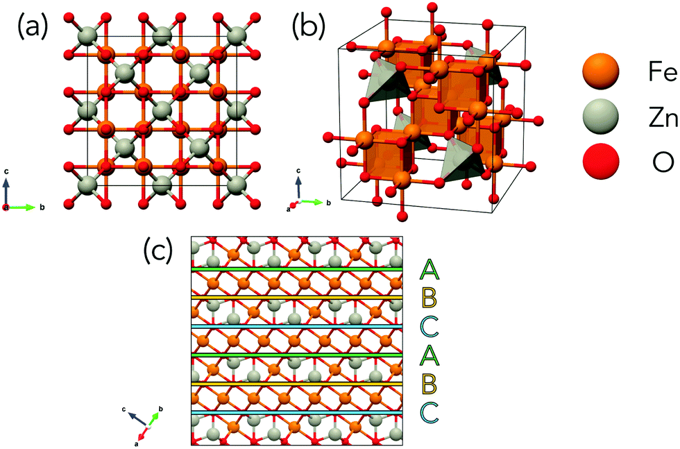Fig. 1 Spinel structure of normal ZnFe₂O₄ in cubic unit cell. (a) Front view of spinel with tetrahedral Zn atoms (grey) between layers of octahedral Fe atoms (orange) and O anions (red). (b) 3D view of cubic spinel. (c) Layers of close-packed O atoms with A (green) B (yellow) and C (blue) layers highlighted. The view in (a) is transformed to the view in (c) by rotation of 45° around the c-axis followed by a rotation of 55° around the bisection of the a-axis and b-axis perpendicular to the c-axis.

Spinels can be disordered over cationic sites by having some of the B³⁺ cations in tetrahedral rather that octahedral sites. The degree of inversion of a spinel describes the extent to which A²⁺ and B³⁺ cations occupy octahedral and tetrahedral sites respectively with the two extremities shown in Fig. 2. A fully normal structure has all occupied tetrahedral sites consisting of A²⁺ cations and all occupied octahedral sites consisting of B³⁺ cations. A fully inverse spinel structure has one-half of occupied octahedral sites filled with A²⁺ cations while the other half is filled with B³⁺ cations and all occupied tetrahedral sites are filled with B³⁺. It is of note that due to the two different species across the octahedral sites in the inverse spinel structure, that there are many possible cation configurations for a fully inverse spinel whereas there is only a single normal configuration. The inversion in spinels results in a very large number of possible configurations.

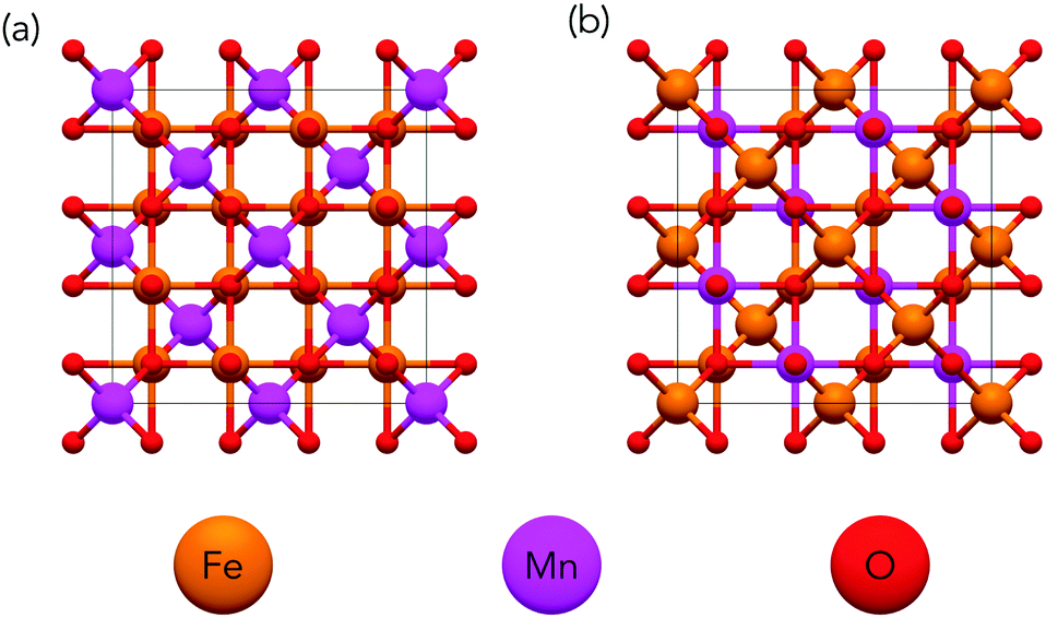Fig. 2 Normal and inverse spinel structures of MnFe₂O₄ in cubic unit cell. The normal structure (a) has all Mn atoms (purple) in tetrahedral sites and all Fe atoms (orange) in octahedral sites. The inverse structure (b) has all Mn atoms in octahedral sites while Fe atoms are distributed over both octahedral and tetrahedral sites.

For a full cubic unit cell with formula A₈B₁₆O₃₂, 24 cations are distributed across 16 octahedral and 8 tetrahedral sites. Using combinatorics there are total of possible cationic configurations. Although this calculation does not include symmetry, assumes unique elements and disregards the distribution of atoms over the tetrahedral sites, the result gives a sense of scale of the number of configurations that need to be considered to fully capture all possible configurations for a simple binary spinel. Table 1 shows the distribution of inversion for structures of a generic A₈B₁₆O₃₂ unit cell generated by random swapping of cations and represents an upper bound of the number of structures. These many possible configurations are possible due to inversion of cations in the structure.

Table 1 Monte-Carlo generation of 57 801 structures showing the distribution of degrees of inversion for a generic spinel full unit cell. The maximum number of structures that could be sampled in this run is 60 000. 2199 structures were rejected due to being equivalent to structures already generated

B^3+tet atoms	Structure count	Percentage of structures
0	1	0.00173
1	7	0.0121
2	265	0.458
3	2462	4.26
4	10 054	17.4
5	19 373	33.5
6	17 607	30.5
7	7027	12.2
8	1005	1.73
Total	57 801	100

---

Pilania and coworkers explore nearly 160 000 spinel configurations in the Mg–Al–Ga–In–O phase field using a cluster-expansion based effective Hamiltonian. Of these, only 350 configurations are explored using DFT methods.³³ This work gives an idea of the scale of DFT calculations that can reasonably be conducted for a given system.

Using DFT methods provides an accurate way to assess the stability of spinel materials but these calculations are computationally intensive and the number than can reasonably be conducted is limited. Therefore, an efficient method for choosing which structures to sample in the composition space is vital to keep the computational cost to a minimum.

One method for searching through configuration space is the ChemDASH methodology presented in the work of Sharp et al.²⁸ ChemDASH uses a basin hopping algorithm to swap atoms in a structure in order to evolve the structure to lower energy configurations. One success using this methodology is presented by Gamon and coworkers as they explore the Li–Al–O–S phase field using ChemDASH, finding the new sulfide Li₃AlS₃.³⁴ Vasylenko and coworkers also use ChemDASH to explore the Li–Sn–S–Cl phase space.³⁵ These works require many runs at different compositions in order to thoroughly explore the phase space which comes with a sizeable computational cost. In the work presented herein, we advance the ChemDASH methodology to allow for multiple variable compositions to be explored in a single run and use this adapted methodology to explore the Zn–Mn–Fe–O spinel phase space.

2 ChemDASH methodology

2.1 Introduction to ChemDASH

ChemDASH is a crystal structure prediction code that uses a chemically-directed atom swapping method to evolve an initial structure. A basin-hopping approach is used to determine acceptance or rejection of a new structure. This methodology allows for efficient exploration of the potential energy surface of a given system. The ChemDASH methodology has been discussed in detail in other publications²⁸ and is briefly reintroduced here.

The ChemDASH work cycle is summarised in Fig. 3. The processes that form this cycle can be reduced to the stages of initialisation, energy minimisation, local environment ranking, atom swapping and structure acceptance. A discussion of each of these stages is given in Note S1 (ESI†).

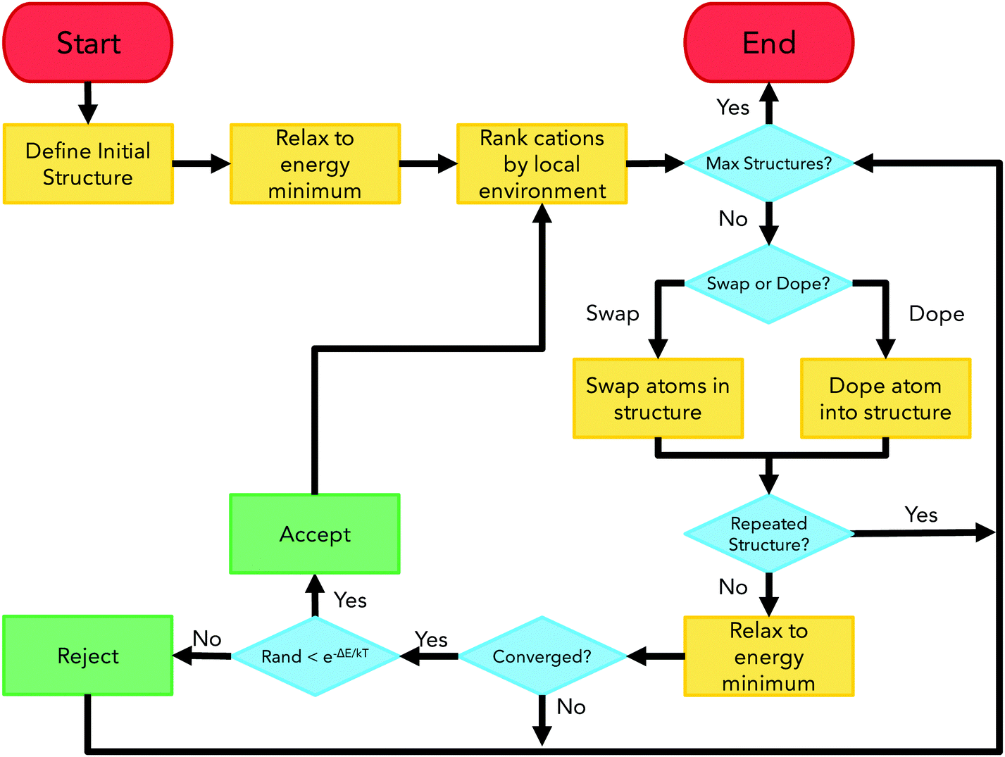Fig. 3 ChemDASH cycle flowchart showing start/end points (red), algorithm actions (orange), decision points (blue) and acceptance/rejection points (green). Figure adapted from Sharp et al.²⁸

2.2 Substitution methodology

To investigate solid solutions with ChemDASH, the methodology has been advanced to allow for variable compositions to be investigated in a single ChemDASH run. Our variable composition version of ChemDASH (vc-ChemDASH) allows for the composition of the structure to be changed at a given ChemDASH step rather than the swapping of atoms already in the structure. The aim of allowing changes in composition is to use information of spinel configurations in similar compositions to efficiently explore both composition and configuration space. In the initial testing presented herein, solid solutions between the ZnFe₂O₄ and MnFe₂O₄ spinel structures are explored using this methodology. This phase space is a good initial test of this methodology as these two systems are both known to be most stable in their normal spinel configurations and the two end members are known to be stable and form a solid solution.

2.2.1 Magnetism. When using ChemDASH with a system containing open-shell transition metal cations, we must carefully consider how we define magnetism in an evolving system. This is important for magnetic spinels as the energy of the system is directly dependent on the magnetic structure. ChemDASH uses the ASE python module³⁶ to define the crystal and magnetic structures and as implemented, each magnetic moment is fixed to each atom object in the system. In many crystal structures however, a swapping of atoms across crystallographic sites does not affect the magnetic structure. This is well described in spinel systems where the Néel magnetic structure (where magnetic moments in tetrahedral and octahedral sites are aligned anti-parallel to one another as shown in Fig. 4a) is found in many magnetic spinel systems over a range of degrees of inversion. Therefore, in this work, each magnetic moment is treated to be fixed to their initial crystallographic sites rather than the atom objects which occupy those sites. The magnitude of each magnetic moment is initially set to ±5 μ_B (depending on site) and allowed to relax to a local energy minimum using density functional theory.

Fig. 4 Ferrimagnetic Neél magnetic structure MnFe₂O₄ (a) and antiferromagnetic magnetic structure of ZnFe₂O₄ (b). The Neél magnetic structure consists of antiferromagnetic coupling of octahedral and tetrahedral sites as shown by the spin up (orange) moments on Fe atoms and spin down (purple) moments on Mn atoms. The antiferromagnetic structure has layers of spin up and spin down moments on Fe atoms.

The end members in the Zn–Mn–Fe–O system have varying magnetic structures due to the nonmagnetic d¹⁰ Zn atoms. MnFe₂O₄ has the ferrimagnetic (FiM) Néel magnetic ordering (shown in Fig. 4a) whereas ZnFe₂O₄ and ZnMn₂O₄ are both antiferromagnetic (AFM) as shown in Fig. 4b. Mn₃O₄ as been shown to have a ferromagnetic ordering below 43 K.³⁷

2.2.2 Substitution pool and random substitution. Substitution in ChemDASH is defined by three parameters: the probability that a substitution event is attempted at any given ChemDASH step, the species in the system that can be doped out, and a pool of possible atoms that can be doped into the system. The substitution pool is defined as a fixed-length list of atoms that each have equal probability of being chosen to be doped in to the structure at a given substitution event. When atom A in the structure is doped out for atom B from the substitution pool, A replaces B in the substitution pool such that the substitution is always reversible. The substitution pool can be of any length, contain any number of unique species and can contain a given species any number of times. Adjusting the relative proportion of different species in the substitution pool effectively allows for weighting of probabilities. The probability of species x_i being chosen as a substituent is therefore equal to the proportion of x_i in the substitution pool.

2.2.3 Energy equivalence. In the original implementation of ChemDASH, the comparison between energies of structures is easily conducted as the composition is unchanged throughout the ChemDASH run. The problem with incorporating variable compositions into ChemDASH is that different chemical compositions do not have directly comparable DFT total energies for use in the acceptance criteria. As implemented here, a solid solution is assumed between two end members that make up the new phase and the energy difference is calculated as the difference between the new structure and the two end members as:

ΔE_ss = E_{(MnxZn1−x)Fe2O4} − (xE_MnFe2O4 + (1 − x)E_ZnFe2O4) (1)

ΔE_ss for the substitution scheme therefore differs from that of the swapping routine as the substitution energy is not dependent on the energy of the previous structure but on the two (stable) end members. When a substitution event occurs then, there is a high likelihood that the energy difference will be positive. This makes acceptance of a substitution event less likely than the acceptance of a swap. Using this energy with the Metropolis criterion allows for the acceptance of substitution with consideration of thermal effects. More advanced implementations such as the energy above the convex hull could also be used to get more accurate relative stabilities, but for this system the solid solution energy is equivalent to the convex hull energy as the spinel disproportionates into the two end members which lie on the convex hull.

2.2.4 Probability of substitution. The modified version of ChemDASH involves assigning a probability to each step for which action is chosen. The substitution_threshold keyword assigns a probability between 0 and 1 that a substitution event occurs at a given step. As this probability is assigned at each step there is no guarantee that proportion of substitution steps over the whole run will be equal to the substitution_threshold. The species chosen from the substitution pool and the species to be doped out are both chosen at random within the constraints of the substitutable_atoms keyword. As a substituent atom is exchanged for the doped out atom, both the substitution pool and the structure will be updated through the ChemDASH run. The probability of each atom in the substitution pool being chosen for a given substitution event is equal and as such a central composition will eventually be found if enough substitution events are accepted.

3 Methods

All DFT calculations were performed using VASP (version 5.4.4).^38–41 The PBE functional⁴² was used with a set of projector-augmented wave pseudopotentials⁴³ (Mn_pv, Fe_pv, Zn, O) for describing core electrons. A plane-wave cut-off energy of 520 eV was used for all calculations with a 3 × 3 × 3 k-point grid. At every ChemDASH step, the structure was relaxed until the total energy is converged to 10⁻⁴ eV and forces on ions converged to 10⁻² eV Å⁻¹. Calculations were performed with spin polarisation to allow for the magnetism of Mn and Fe to be captured. All structures in each ChemDASH step were initialised with the well-known Néel magnetic structure where octahedral and tetrahedral site spins are aligned anti-parallel to one another unless stated otherwise. The current implementation of ChemDASH is written in python3.8 with heavy reliance on the ASE (v3.19) module.³⁶

The variable composition is limited to the ZnFe₂O₄–MnFe₂O₄ (Mn²⁺) phase line as a test case although there is the possibility of Mn³⁺ replacing Fe³⁺ in the structure. This solid solution is shown to be stable in experimental works.^44,45

For the benchmark, ChemDASH runs (without substitution) are performed on all compositions along the Mn²⁺ line (a total of 9 runs). Substitution runs are then compared against these pure swapping runs to analyse how effectively the substitution runs can explore both composition and configuration space. Starting at each end member in their fully normal (ground state) structure and their fully inverse configurations, ChemDASH substitution runs are performed with a maximum of 100 structures sampled where the substitution probability at a given step is set to 0.25, 0.5 and 0.75. This array of probabilities allows us to investigate how the modified algorithm explores the composition and configuration space. The vc-ChemDASH code has been released under the terms of the GNU General Public Licence, and the source code is available at: https://github.com/lrcfmd/vc-ChemDASH. Computational data is available at the University of Liverpool research data catalogue: https://datacat.liverpool.ac.uk.

4 Results

4.1 Original ChemDASH swapping

4.1.1 BVS and random ranking methods. The first test for the methodology to pass is to show that using directed swapping is appropriate for swapping cations in spinel structures. To test the ChemDASH swapping, the BVS and random ranking methods are used on MnFe₂O₄ and ZnFe₂O₄ starting from fully inverse cationic configurations. These calculations are presented in Fig. 5. For MnFe₂O₄ the ground state normal spinel structure is found after 36 steps using the BVS ranking method with most structures lower in energy than the starting structure. For the random swapping the ground state structure is not found in 100 steps. There is a broad range of energies in the structures sampled and many of these are higher in energy than the starting structure. The mean relative energies for the BVS and random swapping runs are 17.8 and 42.0 meV atom⁻¹ respectively showing the bias towards lower energy structures when the BVS method is used. For ZnFe₂O₄ the ground state structure is not found for either BVS or random swapping runs. This is most likely due to the lack of octahedral site preference for Zn. The mean relative energies for BVS and random swapping runs are 21.6 and 28.8 meV atom⁻¹ again showing the bias towards lower energy structures. These tests show that the BVS ranking method in ChemDASH outperforms random swapping in this set-up and is used throughout the rest of the work presented herein.

Fig. 5 Distribution of structure energies for BVS and random swapping ChemDASH runs starting from (a) inverse MnFe₂O₄ and (b) ZnFe₂O₄. Horizontal lines at 39 and 43 meV atom⁻¹ for (a) and (b) respectively show the energy of the starting structure for each run. ΔE_ss is defined relative to the energies of FiM normal MnFe₂O₄ and FiM normal ZnFe₂O₄.

4.1.2 ChemDASH calculations across each composition. For a benchmark to compare our substitution scheme against, each composition along the ZnFe₂O₄–MnFe₂O₄ phase line was run with a pure swapping ChemDASH run (a total of nine runs Zn_xMn_8−xFe₁₆O₃₂ with x = 0–8 at integer intervals). The results are summarised in Fig. 6.

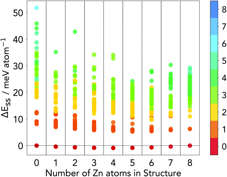Fig. 6 Distribution of energies of structures generated from a ChemDASH run at each composition for Zn_xMn_8−xFe₈O₃₂ where x = 0–8. Points are coloured by the number of Fe atoms in tetrahedral sites in each structure. ΔE_ss is defined relative to the energies of FiM normal MnFe₂O₄ and FiM normal ZnFe₂O₄.

More than 90% of structures shown in Fig. 6 have a low ΔE_ss not exceeding 40 meV atom⁻¹. This shows that in general, compositions along this phase line are stable and at each composition there should be some degree of inversion at finite temperature. Although the magnetic structures of the intermediate compositions may not be the same as the true ground state solutions, the distribution implies that mixing of the two end members is a favourable reaction as the ΔE_ss is small across all compositions. Any magnetic structure that is lower in energy than those assumed here will only make this a more favourable reaction.

There is an obvious energy gap between the lowest energy structure at each composition and all other structures as shown in Fig. 6. From this figure it can be seen that this lowest energy structure for each composition is the fully normal spinel structure (as there are no tetrahedral Fe³⁺ atoms in each lowest energy structure). The small ΔE_ss predicted by ChemDASH for all normal spinel structures shows that these structures are predicted to be thermodynamically stable.

To confirm that the lowest energy structure at each composition does indeed correspond to a stable structure on the convex hull, we calculate the full Mn–Fe–Zn–O convex hull and show all energies in the ESI† (Table S1). The maximum energy difference between ΔE_ss and the convex hull energy is 1.8 meV atom⁻¹. Although some compositions in the solid solution lie above the convex hull at 0 K, these structures are stabilised by the mixing entropy gained by having multiple elements present on the tetrahedral site. The temperature at which the mixing entropy term (ΔS_mixT) is equal to the convex hull energy (E_hull) is shown in Fig. 7 and shows that each structure is stable at 298 K.

Fig. 7 Phase diagram showing the temperature at which ΔS_mixT = E_hull for the normal cation configuration for each composition of Zn_xMn_8−xFe₁₆O₃₂ where x = 0–8 for integer x. The Neél magnetic structure is used for x = 0–6 whereas an AFM ordering is used for x = 7–8 as these yielded the lowest energies. The mixing entropy ΔS_mixT is calculated across tetrahedral sites only as Fe exclusively occupies octahedral sites.

Two clear trends across compositions are evident in Fig. 6. The first is that in general, as the degree of inversion increases, the total energy of the system increases for all compositions. As the two end members are known to be most stable in their normal configurations, it is unsurprising that intermediate compositions follow the same trend. The second trend is that, as the proportion of Zn is increased, higher inversion structures become more stable than similar configurations at other compositions. This is most clearly visible when Fe_tet = 2 and 3 where there is a general decrease in energy going from left to right.

4.1.3 Calculating the degree of inversion. MnFe₂O₄ and ZnFe₂O₄ are known to have a thermally-dependent degree of inversion.^46,47 This is reflected in Fig. 6 as many partially inverse structures are within a thermally accessible energy. At room temperature the thermal energy kT ≈ 25 meV atom⁻¹ and as such configurations lower than this are expected to be accessible at T = 298 K. Higher energy structures can in theory be accessed at higher temperatures and kinetically trapped to allow for higher degrees of inversion. Experimentally this would be shown as a higher average degree of inversion. We can calculate the average inversion for each directed-swapping ChemDASH run using a simple mean.

We can also for a set of randomly generated spinel structures, calculate a Boltzmann-weighted average degree of inversion as another way of modelling the thermally averaged degree of inversion. We calculate the energies of 100 randomly generated cationic configurations of the MnFe₂O₄ and ZnFe₂O₄ end members along with the intermediate composition Mn_0.5Zn_0.5Fe₂O₄. To get a thermally averaged degree of inversion for the three random sets of structures, we calculate a Boltzmann-weighted average inversion using eqn (2):

where A is the degree of inversion for a structure, 〈A〉 is the average inversion over all structures sampled for a single composition and ΔE_i is the solid solution energy ΔE_ss. The thermally-averaged degrees of inversion for MnFe₂O₄, ZnFe₂O₄ and Mn_0.5Zn_0.5Fe₂O₄ are 63.8, 71.3 and 68.4% respectively. These values are very close to the inversion of a random distribution of cations (67%). This shows that, for a small set of structures, that the Boltzmann-weighted average inversion of random structures cannot accurately predict the experimental degree of inversion at 298 K.

The average degree of inversion for MnFe₂O₄ calculated from the directed swapping ChemDASH run (from Fig. 5) is calculated to be 24.6%. This is close to the widely accepted bulk experimental value of 20%^48,49 and a much better estimate than that of the randomly generated structures with thermal averaging. The degree of inversion for ZnFe₂O₄ is calculated to be 50.5% which matches very well with a value of 50% reported by multiple studies^50,51 when the inversion is calculated from the directed-swapping run. The ability to predict physically measurable experimental degrees of inversion with a relatively small sample of structures shows the strength of the combination of directed swapping with the Metropolis acceptance criterion in ChemDASH as applied to spinel materials.

The increasing inversion with Zn addition is corroborated by the experimental results of Sakuri et al. where it is found that in a mixed ZnFe₂O₄–MnFe₂O₄ spinel system, 44% of Zn atoms are in octahedral sites in contrast to the 11% of Mn atoms.⁵² We therefore show here that ChemDASH can be used to predict the degree of inversion for a single spinel composition that can be related to experimental results.

These results from the swapping only ChemDASH show that stable structures for each composition (restricted to those possible in the full unit cell) are readily accessible. For the relatively simple restricted system studied here nine ChemDASH runs are possible with reasonable computational resources, for more complex systems where both A and B cations can be doped out, running ChemDASH at every composition becomes unfeasible. Using a single ChemDASH run at each composition also neglects any relationship between compositions that are similar. The aim of the vc-ChemDASH methodology therefore aims to address both these points by using the relationship between compositions to study the phase space without having to study each composition separately.

4.2 Starting from the normal cationic configuration

Starting from the normal cationic configurations for MnFe₂O₄ and ZnFe₂O₄ the results of each ChemDASH run with elemental substitution are shown in Fig. 8. In Fig. 8a and b the distribution of energies of the ChemDASH run are shown starting from normal MnFe₂O₄ and ZnFe₂O₄.

Fig. 8 Distribution of structure energies for ChemDASH runs starting at normal (a) MnFe₂O₄ and (b) ZnFe₂O₄ with the FiM magnetic structure as a function of the number of Zn atoms in the structure. The results are plotted and coloured by structural index in (c) and (d) to show the evolution of structures over each ChemDASH run. The results are also plotted and coloured by the number of tetrahedral Fe³⁺ atoms (e) and (f) representing the total degree of inversion of each structure. ΔE_ss is defined relative to the energies of FiM normal MnFe₂O₄ and FiM normal ZnFe₂O₄.

For all runs, the energies of the structures do not exceed 35 meV atom⁻¹ above the end members. This energy as compared with the thermal energy k_BT corresponds to T = 406 K which is readily achievable with experimental set-ups. Our calculations use a temperature T = 298 K for the acceptance criteria (kT ≈ 25 meV atom⁻¹). The probability of accepting a structure that is 25 meV atom⁻¹ higher in energy that the previous structure is therefore e⁻¹ ≈ 36.8%.

The low energy structure bias and the small average absolute differences in energies show that the algorithm is able to direct the searching of structures towards plausible low energy structures.

The high substitution regimes (Mn-0.75/Zn-0.75) in Fig. 8 a and b tend to find the ground state structure more often than the lower substitution regimes (Mn-0.25/Zn-0.25) when starting from the normal spinel configuration. This is understood from the normal spinel starting structure being the ground state for all compositions. The higher substitution regime is much more likely to attempt a substitution event at a given step, and therefore the high substitution runs accept many steps in a row finding the normal ground state structures at each composition. The consistent high acceptance rates of swapping (Table 2) implies that, in general, directed swaps either decrease the energy of the structure or increase the energy by only a small amount.

Table 2 Summary of acceptance rates for the vc-ChemDASH runs with different substitution rates starting from FiM normal MnFe₂O₄ and ZnFe₂O₄. A_Total is the total acceptance rate, A_Sub is the acceptance rate of substitution steps and A_Swap is the acceptance rate of swapping steps

	Substitution rate (%)	A Total (%)	A Sub (%)	A Swap (%)
MnFe2O4	25	81.2	53.3	94.3
	50	75.0	58.0	90.0
	75	59.2	50.7	92.6
ZnFe2O4	25	84.2	52.0	98.7
	50	71.6	41.5	91.5
	75	63.3	62.2	73.1

---

The drawback of using higher levels of substitution is clearly shown in Table 2 where the total acceptance rates quickly deteriorate as the substitution level is increased. The individual substitution and swapping acceptance rates are quite stable across different starting structures and substitution levels with substitution steps being much less likely to be accepted than swapping steps.

From the coloured trajectories in Fig. 8c and d it can be seen that the ground state structures are not only found at the start of the ChemDASH run. This is instructive as it shows that due to the bias towards lower energy structures, ground state structures for other compositions can be found after exploration of higher energy composition and configuration space. For each run it is clear that at the start of the run structures of higher energy tend to be sampled before the exploration settles to lower energy, middle composition structures.

Fig. 8e and f shows the number of Fe³⁺ ions in tetrahedral sites and serves as a direct measure of the total degree of inversion for each structure. The structures sampled tend to have low levels of tetrahedral Fe³⁺ with no structure sampled with more than half the tetrahedral sites occupied by Fe³⁺. There is an obvious trend of structures with higher degrees of inversion having high energies relative to the end members. When looking at the structures in the context of octahedral Mn and Zn, there is a preference for having octahedral Zn over octahedral Mn as structures tend to have lower energies (Fig. S1–S6, ESI†). Calculations starting from an intermediate composition (Mn₄Zn₄Fe₁₆O₃₂) yielded results that agree well with those presented in Fig. 8 and are shown in the ESI† (Fig. S7).

The structures with less than 5 Fe³⁺ in tetrahedral sites make up only 19% of all possible structures as shown previously in Table 1. The vc-ChemDASH runs only sample such low inversion configurations, excluding all others. This shows the real strength of the methodology where the structures sampled are focused on low energy regions of space and exclude any structures that are outside this. In the search for stable configurations, being able to exclude a vast region of high energy configuration space is of great use.

The advantage of allowing the composition to change throughout the ChemDASH run is that the feasibility of solid solutions to form between end members can be evaluated. The acceptance of a substitution event shows that in theory a solid solution of that composition should be synthesisable. The more readily substitution events are accepted, the more likely it is that a solid solution will form between the two compositions.

The samples of structures derived from the vc-ChemDASH runs can be mapped to the sample of structures generated from the standard ChemDASH runs where the same regions of configuration space are explored. Given we have already shown the power of ChemDASH in finding low energy structures relative to random swapping, we can conclude that the vc-ChemDASH methodology is a useful extension to ChemDASH for allowing the exploration of both compositional and configurational space. Although the phase space here is relatively simple in that there are only nine different compositions to consider, many chemical spaces are not as simple and could require many more compositions to be tested before adequately sampling the composition space. This extension to ChemDASH allows us to explore the compositional space adequately without resorting to individual ChemDASH runs for all compositions.

4.3 Starting with the AFM magnetic structure

The ground state magnetic structure of ZnFe₂O₄ is AFM and as such ChemDASH runs were also performed using the correct AFM structure for ZnFe₂O₄ starting from normal MnFe₂O₄ and ZnFe₂O₄. For tetrahedral sites, all magnetic moments are aligned in a FM arrangement. The results of this are shown in Fig. 9. As with the FiM vc-ChemDASH runs, the lowest energy ionic configuration for all compositions is the normal cation configuration (Fig. 9a and b).

Fig. 9 (a) and (b) show the distribution of structure energies for ChemDASH runs starting at normal (a) MnFe₂O₄ and (b) ZnFe₂O₄ with the AFM magnetic structure as a function of the number of Zn atoms in the structure. Runs with 25% (left), 50% (central) and 75% (right) are plotted and each run is coloured by structure index to show the evolution of each ChemDASH run. (c) The distribution of structure energies relative to FiM-MnFe₂O₄ and FiM-ZnFe₂O₄ show the differences in total energy between FiM and AFM magnetic structures as each ChemDASH run evolves. Each coloured data set is the aggregate of the 25, 50 and 75% substitution rates. ΔE_ss is defined relative to the energies of AFM normal MnFe₂O₄ and AFM normal ZnFe₂O₄.

Comparison of the energies of the AFM and FiM runs are presented in Fig. 9c with relative energies defined relative to FiM normal MnFe₂O₄ and AFM normal ZnFe₂O₄. For all compositions except N_Zn = 7 or 8 the ground state structure is most stable in the FiM runs than the AFM runs. This shows a collapse of the AFM magnetic structure upon addition of a small amount of Mn to the unit cell. Looking at the whole collection of sampled structures shows that when any inversion is introduced, even for N_Zn = 7 or 8, structures have a lower energy in the FiM state than the AFM state.

Even with the higher and wider range of energies for the AFM runs, the sample of structures obtained from the AFM runs are similar to those of the FiM runs and the swapping-only runs. The acceptance rates for AFM runs are also very similar to those of FiM runs (Table S1, ESI†). Although the algorithm is robust to using different magnetic structures, it seems that for this system that the FiM set-up is a more appropriate choice to use for finding new spinel configurations and compositions.

An interesting observation is that due to the change in magnetic symmetry, the normal spinel configuration no longer has only one unique magnetic structure for any of the mixed composition spinels (i.e. excluding MnFe₂O₄ and ZnFe₂O₄). This is due to the two unique layers of tetrahedral sites that can either be between FM aligned octahedral layers or AFM aligned octahedral layers (see Fig. 4b). As mixing of the two end members reaches an equimolar mix of Mn and Zn, many unique normal structures are possible. When the magnetic structure is changed to the FiM structure, these unique structures collapse to the same equivalent structure. This is most clearly observed in Fig. 9a where multiple different normal spinels are observed for N_Zn = 2–5. An extensive discussion of magnetism in spinels is presented by Tsurkan and coworkers.⁵³

4.4 Starting with the fully inverse cation configuration

Starting from the fully inverse cation configuration presents a much more difficult challenge for the methodology. The fully inverse structure for both MnFe₂O₄ and ZnFe₂O₄ are the furthest cation configurations from the ground state and so present a worst-case scenario for looking at unknown phase fields. The distribution of structures in terms of degree of inversion (Table 1) also presents a challenge as there are far fewer low inversion structures than there are high inversion structures which makes finding the normal ground state difficult at any composition.

The inverse structures at the start of each set of runs have much higher energies than the ground state (38.7 meV atom⁻¹ for MnFe₂O₄ and 45.2 meV atom⁻¹ for ZnFe₂O₄). As the run progresses, the energy of the structure decreases quite rapidly until only the lowest energy structures are sampled. In Fig. 10a and b, the trajectory clearly shows that for each run the energy of the system decreases as the run progresses and after 20 steps does not increase to an energy above 30 meV atom⁻¹ with structures where Fe_tet > 4 no longer sampled. Across all 6 runs conducted starting from inverse structures, no substitution events are accepted directly from the initial structure. For MnFe₂O₄ and ZnFe₂O₄ starting runs, substitution steps are not accepted until cations are swapped to lower the energy to below 20 and 30 meV atom⁻¹ respectively (relative to the ground state end members).

Fig. 10 Distribution of structure energies for ChemDASH runs starting at inverse (a) MnFe₂O₄ and (b) ZnFe₂O₄ with the FiM magnetic structure as a function of the number of Zn atoms in the structure. Runs with 25% (left), 50% (central) and 75% (right) are plotted and each run is coloured by structure index to show the evolution of each ChemDASH run. The results are also plotted coloured by the number of tetrahedral Fe³⁺ atoms (c and d) representing the total degree of inversion of each structure. ΔE_ss is defined relative to the energies of FiM normal MnFe₂O₄ and FiM normal ZnFe₂O₄.

Across all substitution levels the energy of the system decreases as the run progresses. The Mn-0.25 and Mn-0.50 runs find the normal ground state structures for N_Zn = 4, 5. By finding the ground state, it is shown that the algorithm can start from the highest energy structure possible and evolve the system to find the lowest energy structure. The ground state is not found for the Mn-0.75, most probably due to the small number of swapping steps attempted in the 100 structure run. The true ground state is also not found starting from the inverse ZnFe₂O₄ structure although many structures with 1 tetrahedral Fe atom are found (Fig. 10). This suggests that more than 100 structures may need to be sampled in order to find the true ground state structure.

In Fig. 10c and d, the degree of inversion decreases very quickly with very few high inversion structures sampled. This shows the benefit of using the BVS method in ChemDASH to direct swaps away from high energy, high inversion structures to lower energy, low inversion structures. It is also informative that the majority of structures sampled starting from the inverse structures are in the same composition and configuration space as those of the normal-start runs. This shows that the structures sampled throughout the run are independent of the starting ionic configuration given sufficient steps for the run to equilibrate. The ability of the algorithm to operate well even when starting from high energy structures is essential for use in new and unknown phase spaces.

5 Solid solution properties

Having looked at how the new implementation of ChemDASH works with the types of structures it samples, the properties of the solid solution can be analysed. Not only does this serve as an investigation of the Mn–Fe–Zn–O spinel phase space but also provides a template for analysing ChemDASH runs.

The radial distribution function (RDF) in Fig. 11 for metal–metal and metal–oxygen distances of all accepted structures starting from the normal FiM structures (as presented in Section 4.2) are shown in Fig. 11a and b. Fig. 11a shows the intermetallic distances for octahedral–octahedral (3.05 Å), octahedral–tetrahedral (3.55 Å) and tetrahedral–tetrahedral (3.70 Å) sites. The peaks at 3.05 Å and 3.55 Å highlight the abundance of Fe in octahedral sites while the peak at 3.70 Å highlights the abundance of Mn and Zn in tetrahedral sites. Fig. 11b shows a clear distinction between Zn atoms in octahedral (2.01 Å) and tetrahedral (2.14 Å) sites. The same observation can be made for the Fe–O bond lengths in tetrahedral (1.93 Å) and octahedral sites (2.05 Å). The octahedral site peak (2.05 Å) is dominant for Mn and the tetrahedral peak at 2.19 Å is barely resolvable.

Fig. 11 Radial distribution functions of metal–oxygen M–O (a) and metal–metal M–M (b) distances for vc-ChemDASH runs starting with normal FiM starting structures. Distribution of energies as a function of average M–O octahedral bond lengths (c) and tetrahedral bond lengths (d).

A comparison of average bond lengths of each metal in octahedral and tetrahedral sites is shown in Fig. 11c and d. In general, the trend of M–O bond lengths holds where Mn–O > Zn–O > Fe–O for both octahedral and tetrahedral sites. There are however some clear outliers for the average octahedral and tetrahedral bond lengths. These outliers have smaller average Mn–O octahedral and larger Fe–O tetrahedral bond lengths than the majority of Mn and Fe sites and make up 4.3% of all structures sampled. To further investigate the origin of these outliers, the data was split into the majority of structures and the subset of outliers for subsequent analysis.

Looking at the magnetic moments of the minority subset shows deviations from the expected d⁵ Mn²⁺ and Fe³⁺ configurations. For each structure in the subset there is a coupling between an octahedral Mn and tetrahedral Fe resulting in a lowering of the overall magnetic moment of both the Mn and Fe. For all structures these sites are direct neighbours as shown in Fig. 13. The average magnitude of the magnetic moment for octahedral and tetrahedral Fe sites is 4.2 μ_B in the non-coupled sites. The average magnetic moment decreases significantly to 3.7 μ_B in the coupled subset. For Mn, the average magnitude of magnetic moments are 4.6 μ_B for octahedral and tetrahedral sites of the non-coupled structures. The average magnetic moment is again decreased for the coupled subset to 3.9 μ_B. The origin of this can be attributed to an oxidation of Mn²⁺ to Mn³⁺ and a reduction of Fe³⁺ to Fe²⁺.

The projected density of states for a representative coupled and non-coupled structure are presented in Fig. 12. Each structure has four Mn atoms and four Zn atoms and each has one Mn in an octahedral site. The octahedral Mn states in Fig. 12a show a single unoccupied low energy unoccupied state in the spin-up channel as would be expected in a d⁴ Mn³⁺ cation. The two high energy occupied states in the spin-up channel of the non-coupled structures (Fig. 12b) correspond to the two higher energy filled states in the high-spin d⁵ electronic configuration of Mn²⁺.

Fig. 12 Projected density of states for coupled and non-coupled structures. Projected density of states for Mn in coupled (a) and non-coupled (b) structures. Project density of states for Fe in coupled (c) and non-coupled (d) structures.

Fig. 13 (a) Example structure of the coupling between tetrahedral Fe (orange tetrahedron) and octahedral Mn (purple octahedron). (b) Mn octahedron with bond lengths showing distortion of structure. (c) Fe tetrahedron.

Fig. 12c distinguishes Fe²⁺ and Fe³⁺ in different tetrahedral sites and shows the difference in electronic density of states between the two sites. The Fe²⁺ site has a single high-energy occupied state as would be expected for a high-spin Fe²⁺ d⁶ cation. The Fe³⁺ tetrahedral site density of states in the coupled structure matched that of the tetrahedral Fe in the non-coupled structure (Fig. 12c) with no high-energy filled states in the spin-up channel. The distortion of the minority subset is therefore attributed to Jahn–Teller distortion of the Fe²⁺ and Mn³⁺ metal cations. This confirms the coupling nature of the subset of distorted structures allowing for some Mn³⁺ and Fe²⁺ to be present in the system.

Experimentally, there are various reports of the presence of Mn³⁺ and Fe²⁺ in the Mn–Fe–Zn–O spinel phase field. Harrison and coworkers⁵⁴ determine for a sample of MnFe₂O₄ that approximately 7% of Fe is in the Fe²⁺ state and 17% of Mn is in the Mn³⁺ state. Ji and coworkers⁵⁵ find a Zn-doped MnFe₂O₄ with a slight excess of Fe resulting in approximately 3% of Fe in the Fe²⁺ state with Ti⁴⁺ doping increasing the amount of Fe²⁺ up to 6%. Bonsdorf and coworkers⁵⁶ find a temperature dependence for the Mn²⁺/Mn³⁺ ratio where high temperature processing forms Mn²⁺ exclusively. Their work however finds no existence of Fe²⁺ using Mössbauer spectroscopy. Carta and coworkers⁴⁷ argue that in a pure sample of MnFe₂O₄, a highly inverted structure (≈70% inversion) is attributed to partial oxidation of Mn²⁺ to Mn³⁺. Antic and coworkers⁴⁵ on the other hand show cation deficit Zn–Mn ferrites where they observe no Mn³⁺ but claim the presence of Mn⁴⁺. They also find Fe²⁺ in small quantities. These experimental reports suggest that the presence of Mn³⁺ and Fe²⁺ in Zn–Mn ferrite spinels is certainly possible but that this is strongly dependent on synthesis methods and conditions. It is noted that the orbital occupancies and magnetic moments calculated by the DFT+U approach used in our study will depend on the value of U used.⁵⁷ Nevertheless, our results are consistent with experimental reports of the presence of Fe²⁺ and Mn³⁺ in members of this solid solution.

This section highlights the physical properties that can be obtained across an entire spinel phase space using the new vc-ChemDASH methodology. From this trends and properties such as inversion degree, cation charges, etc. can be determined before more refined ChemDASH calculations on specific compositions can be conducted. This new methodology therefore allows for broad properties of the spinel phase space to be predicted in a single ChemDASH calculation.

6 Conclusions

We have presented here developments to the ChemDASH methodology allowing for the consideration of magnetic structures and the variation of the composition of a system during a ChemDASH run. We show that the original ChemDASH methodology is an efficient search algorithm for finding low energy configurations of spinels in the Mn–Fe–Zn–O phase field. From this, we show that the new variable composition methodology can be used to assess the likelihood that a solid solution forms between two end members without having to assess all compositions individually. By reducing the number of structures that need to be assessed, this methodology provides an efficient search in both composition and chemical space. We also show that this methodology works well with different magnetic structures and starting configurations ideal for evaluating unknown composition spaces in solid solutions between materials. It is envisaged that this methodology will be used to evaluate solid solutions in other structure types (e.g. perovskites) beyond spinels to find new materials with functional properties.

Conflicts of interest

There are no conflicts to declare.

Acknowledgements

We thank Johnson-Matthey for the funding of the PhD studentship for Robert Dickson. We would also like to thank the University of Liverpool for computing resources on Barkla. This work used the Cirrus UK National Tier-2 HPC Service at EPCC (http://www.cirrus.ac.uk) funded by the University of Edinburgh and EPSRC (EP/P020267/1) and the national HPC resource, Archer, provided through the EPSRC program grant (EP/N004884/1).

Notes and references

1. S. Kim, M. Lee, C. Hong, Y. Yoon, H. An, D. Lee, W. Jeong, D. Yoo, Y. Kang, Y. Youn and S. Han, Sci. Data, 2020, 7, 1–6.
2. S. You, S. Li, L. Wang, T. Takeda, N. Hirosaki and R. J. Xie, Chem. Eng. J., 2021, 404, 126575.
3. S. Adachi, J. Lumin., 2018, 202, 263–281.
4. B. T. Matthias, T. H. Geballe and V. B. Compton, Rev. Mod. Phys., 1963, 35, 1–22.
5. T. Hirakawa, Y. Shimokawa, W. Tokuzumi, T. Sato, M. Tsushida, H. Yoshida, S. Hinokuma, J. Ohyama and M. MacHida, ACS Catal., 2019, 9, 11763–11773.
6. A. Cimino and F. S. Stone, Adv. Catal., 2002, 47, 141–306.
7. M. Schmidt, T. Stumpf, M. M. Fernandes, C. Walther and T. Fanghänel, Angew. Chem., Int. Ed., 2008, 47, 5846–5850.
8. A. K. Singh and A. Subramaniam, J. Alloys Compd., 2014, 587, 113–119.
9. C. Gente, M. Oehring and R. Bormann, Phys. Rev. B: Condens. Matter Mater. Phys., 1993, 48, 13244–13252.
10. P. Porta, S. De Rossi, M. Faticanti, G. Minelli, I. Pettiti, L. Lisi and M. Turco, J. Solid State Chem., 1999, 146, 291–304.
11. M. Trari, J. Töpfer, P. Dordor, J. C. Grenier, M. Pouchard and J. P. Doumerc, J. Solid State Chem., 2005, 178, 2751–2758.
12. M. Isobe and Y. Ueda, J. Alloys Compd., 2004, 383, 85–88.
13. A. Rothschild, W. Menesklou, H. L. Tuller and E. Ivers-Tiffée, Chem. Mater., 2006, 18, 3651–3659.
14. F. R. Sensato, R. Custodio, E. Longo, A. Beltrán and J. Andrés, Catal. Today, 2003, 85, 145–152.
15. C. Battistoni, J. L. Dormann, D. Fiorani, E. Paparazzo and S. Viticoli, Solid State Commun., 1981, 39, 581–585.
16. A. K. Cheetham and D. A. O. Hope, Phys. Rev. B: Condens. Matter Mater. Phys., 1983, 27, 6964–6967.
17. M. Polomska, W. Kaczmarek and Z. Pajak, Phys. Status Solidi, 1974, 23, 567–574.
18. M. Mahesh Kumar, S. Srinath, G. S. Kumar and S. V. Suryanarayana, J. Magn. Magn. Mater., 1998, 188, 203–212.
19. A. Z. Menshikov, Y. A. Dorofeev, A. G. Klimenko and N. A. Mironova, Phys. Status Solidi, 1991, 164, 275–283.
20. Z. Y. Zhao, Q. L. Liu and W. W. Dai, Sci. Rep., 2016, 6, 1–12.
21. C. Yang and Z. Y. Zhao, J. Am. Ceram. Soc., 2019, 102, 4976–4989.
22. I. Grinberg, M. R. Suchomel, W. Dmowski, S. E. Mason, H. Wu, P. K. Davies and A. M. Rappe, Phys. Rev. Lett., 2007, 98, 107601.
23. J. S. Bechtel and A. Van Der Ven, Phys. Rev. Mater., 2018, 2, 1–7.
24. A. Udyansky, J. Von Pezold, A. Dick and J. Neugebauer, Phys. Rev. B: Condens. Matter Mater. Phys., 2011, 83, 184112.
25. L. Li, J. T. Muckerman, M. S. Hybertsen and P. B. Allen, Phys. Rev. B: Condens. Matter Mater. Phys., 2011, 83, 134202.
26. A. R. Oganov and C. W. Glass, J. Chem. Phys., 2006, 124, 244704.
27. C. W. Glass, A. R. Oganov and N. Hansen, Comput. Phys. Commun., 2006, 175, 713–720.
28. P. M. Sharp, M. S. Dyer, G. R. Darling, J. B. Claridge and M. J. Rosseinsky, Phys. Chem. Chem. Phys., 2020, 22, 18205–18218.
29. P. Raiteri, A. Laio, F. L. Gervasio, C. Micheletti and M. Parrinello, J. Phys. Chem. B, 2006, 110, 3533–3539.
30. Q. Zhu, A. R. Oganov and A. O. Lyakhov, Comput. Phys. Commun., 2006, 124, 227.
31. J. Pannetier and V. Caignaeru, Nature, 1990, 346, 343–345.
32. Y. Wang, J. Lv, L. Zhu and Y. Ma, Phys. Rev. B: Condens. Matter Mater. Phys., 2010, 82, 094116.
33. G. Pilania, V. Kocevski, J. A. Valdez, C. R. Kreller and B. P. Uberuaga, Commun. Mater., 2020, 1, 1–11.
34. J. Gamon, B. B. Duff, M. S. Dyer, C. Collins, L. M. Daniels, T. W. Surta, P. M. Sharp, M. W. Gaultois, F. Blanc, J. B. Claridge and M. J. Rosseinsky, Chem. Mater., 2019, 31, 9699–9714.
35. A. Vasylenko, J. Gamon, B. B. Duff, V. V. Gusev, L. M. Daniels, M. Zanella, J. F. Shin, P. M. Sharp, A. Morscher, R. Chen, A. R. Neale, L. J. Hardwick, J. B. Claridge, F. Blanc, M. W. Gaultois, M. S. Dyer and M. J. Rosseinsky, Nat. Commun., 2021, 12, 5561.
36. A. Hjorth Larsen, J. Jørgen Mortensen, J. Blomqvist, I. E. Castelli, R. Christensen, M. Dułak, J. Friis, M. N. Groves, B. Hammer, C. Hargus, E. D. Hermes, P. C. Jennings, P. Bjerre Jensen, J. Kermode, J. R. Kitchin, E. Leonhard Kolsbjerg, J. Kubal, K. Kaasbjerg, S. Lysgaard, J. Bergmann Maronsson, T. Maxson, T. Olsen, L. Pastewka, A. Peterson, C. Rostgaard, J. Schiøtz, O. Schütt, M. Strange, K. S. Thygesen, T. Vegge, L. Vilhelmsen, M. Walter, Z. Zeng and K. W. Jacobsen, J. Phys. Condens. Matter, 2017, 29, 273002.
37. R. B. B. Boucher and M. Perrin, J. Appl. Phys., 1971, 42, 1615.
38. G. Kresse and J. Hafner, Phys. Rev. B: Condens. Matter Mater. Phys., 1993, 47, 558–561.
39. G. Kresse and J. Hafner, Phys. Rev. B: Condens. Matter Mater. Phys., 1994, 49, 14251–14269.
40. G. Kresse and J. Furthmüller, Comput. Mater. Sci., 1996, 6, 15–50.
41. G. Kresse and J. Furthmiiller, Phys. Rev. B, 1996, 54, 11169–11186.
42. J. P. Perdew, K. Burke and M. Ernzerhof, Phys. Rev. Lett., 1996, 77, 3865–3868.
43. D. Joubert, Phys. Rev. B: Condens. Matter Mater. Phys., 1999, 59, 1758–1775.
44. B. K. Argymbek, S. E. Kichanov, D. P. Kozlenko, E. V. Lukin, A. T. Morchenko, S. G. Dzhabarov and B. N. Savenko, Phys. Solid State, 2018, 60, 1727–1732.
45. B. Antic, A. Kremenović, A. S. Nikolic and M. Stoiljkovic, J. Phys. Chem. B, 2004, 108, 12646–12651.
46. L. I. Granone, A. C. Ulpe, L. Robben, S. Klimke, M. Jahns, F. Renz, T. M. Gesing, T. Bredow, R. Dillert and D. W. Bahnemann, Phys. Chem. Chem. Phys., 2018, 20, 28267.
47. D. Carta, M. F. Casula, G. Mountjoy and A. Corrias, Phys. Chem. Chem. Phys., 2008, 10, 3108–3117.
48. F. H. Martins, F. G. Silva, F. L. O. Paula, J. D. A. Gomes, R. Aquino, J. Mestnik-Filho, P. Bonville, F. Porcher, R. Perzynski and J. Depeyrot, J. Phys. Chem. C, 2017, 121, 8982–8991.
49. K. Vamvakidis, M. Katsikini, D. Sakellari, E. C. Paloura, O. Kalogirou and C. Dendrinou-Samara, Dalton Trans., 2014, 43, 12754–12765.
50. M. A. Cobos, P. De La Presa, I. Llorente, J. M. Alonso, A. Garciá-Escorial, P. Marín, A. Hernando and J. A. Jiménez, J. Phys. Chem. C, 2019, 123, 17472–17482.
51. R. Sai, S. D. Kulkarni, S. S. Bhat, N. G. Sundaram, N. Bhat and S. A. Shivashankar, RSC Adv., 2015, 5, 10267–10274.
52. S. Sakurai, S. Sasaki, M. Okube, H. Ohara and T. Toyoda, Phys. B: Condens. Matter, 2008, 403, 3589–3595.
53. V. Tsurkan, H. A. Krug von Nidda, J. Deisenhofer, P. Lunkenheimer and A. Loidl, Phys. Rep., 2021, 926, 1–86.
54. F. W. Harrison, W. P. Osmqnd and R. W. Teale, Phys. Rev., 1957, 106, 865–866.
55. H. Ji, Z. Lan, Z. Xu, H. Zhang and G. J. Salamo, IEEE Trans. Magn., 2013, 49, 4277–4280.
56. G. Bonsdorf, Solid State Ionics, 1997, 101–103, 351–357.
57. C. Li, P. Li, L. Li, D. Wang, X. Gao and X. J. Gao, RSC Adv., 2021, 11, 21851–21856.

---

Footnote

† Electronic supplementary information (ESI) available. See DOI: https://doi.org/10.1039/d2cp02180c

---