
 Open Access Article
 This Open Access Article is licensed under a
 Creative Commons Attribution 3.0 Unported Licence
Interaction between two polyelectrolytes in monovalent aqueous salt solutions†
Xiang
Yang
 *a,
Alberto
Scacchi
abc,
Hossein
Vahid
abc,
Maria
Sammalkorpi
bcd and
Tapio
Ala-Nissila
aef
*a,
Alberto
Scacchi
abc,
Hossein
Vahid
abc,
Maria
Sammalkorpi
bcd and
Tapio
Ala-Nissila
aef
aDepartment of Applied Physics, Aalto University, P.O. Box 11000, FI-00076 Aalto, Finland. E-mail: xiang.yang@aalto.fi
bDepartment of Chemistry and Materials Science, Aalto University, P.O. Box 16100, FI-00076 Aalto, Finland
cAcademy of Finland Center of Excellence in Life-Inspired Hybrid Materials (LIBER), Aalto University, P.O. Box 16100, FI-00076 Aalto, Finland
dDepartment of Bioproducts and Biosystems, Aalto University, P.O. Box 16100, FI-00076 Aalto, Finland
eQTF Center of Excellence, Department of Applied Physics, Aalto University, P.O. Box 11000, FI-00076 Aalto, Finland
fInterdisciplinary Center for Mathematical Modelling and Department of Mathematical Sciences, Loughborough University, Loughborough, Leicestershire LE11 3TU, UK
First published on 26th August 2022
Abstract
We use the recently developed soft-potential-enhanced Poisson–Boltzmann (SPB) theory to study the interaction between two parallel polyelectrolytes (PEs) in monovalent ionic solutions in the weak-coupling regime. The SPB theory is fitted to ion distributions from coarse-grained molecular dynamics (MD) simulations and benchmarked against all-atom MD modelling for poly(diallyldimethylammonium) (PDADMA). We show that the SPB theory is able to accurately capture the interactions between two PEs at distances beyond the PE radius. For PDADMA positional correlations between the charged groups lead to locally asymmetric PE charge and ion distributions. This gives rise to small deviations from the SPB prediction that appear as short-range oscillations in the potential of mean force. Our results suggest that the SPB theory can be an efficient way to model interactions in chemically specific complex PE systems.
1 Introduction
Polyelectrolytes (PEs) are polymers containing electrolyte groups, which dissociate in aqueous solutions into solvated counterions and charged polymers. PEs exhibit physical properties very different from those of the uncharged polymers, in particular in terms of their aqueous solubility and tunability with salt.1,2 Consequently, PE solutions and PE assemblies strongly react to changes in solvent environment, temperature, pH, and salt conditions.3–5 When their molecular persistence length is long enough, PEs can be considered, to some extent, as charged rods. Examples of such PEs include, e.g., functionalized cellulose fibrils, tobacco mosaic virus, DNA, and actin. The interactions between rod-like PEs are widely addressed in chemistry and biology, leading to both rich functional and assembly behavior, such as in complex assembly of DNA and RNA,6,7 cellulose nanocrystal based advanced self-assembly,8,9 and complexation based synthetic PE materials.3,10 The extensive applications of PEs in the field of nanostructured materials span from responsive materials,3 surface modification11 to layer-by-layer assembly.12,13The fundamentals to understanding self-assembly, as well as structural and dynamical properties of dense PE systems, to a first approximation, come from the PE-PE pairwise interactions. These interactions in ionic solutions are however complex due to effects rising from both charge correlations and solution conditions. Replacing atomistically detailed models with lower resolution, coarse-grained (CG) counterparts have paved the way to efficiently study and simulate large-scale processes at time scales inaccessible to all-atom models.14,15 To this end, it is beneficial to consider simplified geometries, such as assuming rod-like, rigid PEs, axially symmetric charge distributions, and simplified descriptions of ions in the solution around the charged species.
The mean-field Poisson–Boltzmann (PB) theory has proven to be efficient in describing the condensation of monovalent ions around single low-charge rods.16–21 This theory is able to predict various properties of PE solutions including electrophoretic migration, surface adsorption and osmotic pressure, for a wide range of concentrations.22–24 However, PB theory fails when charge correlations become strong, such as for high ion valency, high surface-charge density, and low temperatures. There exists an extensive literature on the effects of charge correlations on ion condensation for PEs beyond the mean-field PB theory.25–28 Perhaps the most striking effect of such correlations is the reversal of the effective PE charge for multivalent counterions, which also reverses the field-driven PE mobility.26,29 Additionally, the PB theory treats mobile ions as point charges. Successful models incorporating ion size effect exist, such as those in ref. 30 and 31.
Another shortcoming of these simplified models is that PEs, such as DNA or charged polypeptides, are atomistically structured, exhibiting a local spatially inhomogeneous charge distribution. The details of the local structure are however important and affect both the persistence length,32,33 the charge distribution around the PE, and the PE interactions.34,35
Ion condensation and salt solution response of PEs are also salt species and PE dependent.34,35 Such dependencies can, to some degree, be captured by an empirical modifications of the PB theory.21,36
In systems consisting of two rod-like PEs, PB theory has also been often applied, in particular in the case of monovalent salt solutions. The interaction between two charged cylinders has been calculated in many theoretical works with different boundary conditions and approximations.37–40 The linear version of PB theory with the Debye–Hückel approximation (LPB) provides an explicit analytical solution of the interaction between two parallel cylinders.41–43 However, LPB theory fails in dealing with highly charged molecules or small cylinder radii (as comparable to the Debye length), such as, e.g., in the case of DNA.37 Charge correlations in the strong-coupling regime lead to like-charge attraction.44–51 For dense PE systems, the attraction induces, e.g., bundle formation of F-actin and toroidal aggregates of concentrated DNA.12,52
Recently, we have developed a soft-potential-enhanced PB (SPB) theory to efficiently and accurately compute ion density distributions in the weak-coupling regime.53 The soft potential in the SPB theory contains only one (physical) parameter, which can be fixed to give a good description for monovalent ion densities and electrostatic potentials around single rodlike PE for a wide range of salt and ion sizes. The SPB approach was shown to work well for monovalent salt concentrations up to 1 M and ion sizes ranging from those corresponding to small, hard monovalent ions, such as Na+ and Cl−, to almost an order of magnitude larger ions with diameter comparable to the PE diameter.53 These results constitute a significant improvement over the standard PB approach, and thus we expect that the SPB approach could be used for modeling systems with multiple PEs present.
To this end, encouraged by the success of the SPB theory, in the present work we apply it to compute the ion distributions and corresponding PE–PE interactions via the potential-of-mean-force calculation for two rodlike PEs in the weak-coupling regime. We compare the SPB modelling outcome against a chemically specific PE. To this end, we choose a relatively high-charge-per-length cationic and very common polyelectrolyte poly(diallyldimethylammonium) (PDADMA) as the PE focus of the study. PDADMA is chosen because of its technological relevance in, e.g., water purification, flocculation, and paper industry.54 Furthermore, the strong amide charges can be expected to cause localization, i.e. deviations from the mean field predictions.
The SPB theory is first benchmarked against molecular dynamics (MD) simulations of a CG model of PDADMA PE in salt solution, which allows the SPB fitting parameter to be optimized and fixed. We obtain good agreement between the mean-field and coarse-grained models in capturing the interactions between two PEs. To further elaborate the influence of the atomic structure of the PE, we show by atomistic-detail MD simulations of PDADMA how positional dependencies between the charged groups induce correlation in the ion distribution. For the simulation setup in which the atomistic-detail PE is stretched straight, these emerge as asymmetric, helical configurations. Such positional correlations in the ion distribution lead to small deviations from the SPB and CG model predictions in interaction strength and show as short-range deviation from the PB smooth prediction in the potential of the mean force.
In the case of DNA, which also exhibits a helical molecular structure, DNA–DNA interactions can be split into two types of contributions.55 The first one comprises non-specific interactions such as electrostatics and the hydration force which allow the treatment of DNA as featureless rod, while the second contribution depends on the helical structure and its sequence. In solution, DNA is surrounded by a variety of charged molecules, ranging from small metal ions to polyions. Flexible linear multivalent ions, such as spermidine (3+) and spermine (4+), are widely used as DNA-condensing agents.52 It has been shown that the aggregation of DNA decreases with the addition of monovalent salt.56 In the presence of larger cationic polymers, hexagonal packing of DNA is observed for DNA complexed with polycations.57 The double helices come close to each other in the condensed phase, leading to the restructuring of water molecules, giving rise to so-called hydration forces.55,58 The general features of the DNA phase transition are mainly determined by non-specific properties; in addition to electrostatic interactions and hydration force, also DNA length, concentration and temperature play an important role.59 In contrast, the specific DNA sequence determines local interactions and recognition between the double helices in the condensed DNA phase.60 Details of the helical structure are thus the key in analysing the transition from hexagonal arrays to cholesteric packing.61
The manuscript is organized as follows: Section 2 introduces the different methodologies used in this work. Specifically, in Section 2.1 we describe our all-atom MD simulations, in Section 2.2 the CG-MD simulations, and in Section 2.3 the SPB theory. In Section 3.1 we present the results regarding the SPB model parametrized against CG-MD simulations and compare the different models against the all-atom MD simulations. We discuss the ion density distributions predicted by the different approaches, underpinning the effect of the atomistic structure of the PE. Furthermore, in Section 3.2 we show good agreement between PE–PE interactions, as captured by the potential of mean force between two parallel PEs corresponding to PDADMA in monovalent salt solution obtained from the different description levels. Finally, in Section 4 we summarize our findings and provide prospects for the application of SPB to model chemically specific complex PE systems.
2 Methods
2.1 Atomistic molecular dynamics simulations
The system setup is shown in Fig. 1(a and b) where the atomistic-detail MD simulations include either one or two linear PE chains set to span the cuboid simulation box along the z axis as periodic chains (terminal group connected over the periodic boundary condition). The initial configuration preparation protocol follows ref. 21 and leads to infinite, straight PE chains (covalently bonded over the periodic boundary). The stretched PE configuration is used as a simplification, enabling direct comparison with PB theory for cylindrical objects. In comparison, a free-ended PDADMA chain fluctuates in backbone conformations, which influences both ion distribution and complexation with oppositely charged PEs, see e.g. ref. 62–65. | ||
| Fig. 1 (a and b) Initial simulation snapshots of the all-atom MD simulations with (a) one and (b) two PDADMA chains in a 7.9 × 7.9 × 5.66 nm3 simulation box. For clarity, the explicit water in the simulations is omitted in these visualizations. (c and d) Initial simulation snapshots of the CG MD simulations of (c) one and (d) two CG models of PDADMA-like PEs in a 20 × 20 × 20 nm3 simulations box. σB is the effective bead diameter of PDADMA in the CG model, which has implicit solvent. In (a–d), the added salt concentration is 0.26 M, and the Na+ and Cl− ions are green and yellow, respectively. (e) A close-up view of the atomistic-detail structure of the straight PDADMA chain and the chemical structure of a monomer of PDADMA. In the atomistic structure, the N+, C and H atoms (here spheres) are colored in red, blue, and gray, respectively. A z axial straight line visualizes the PE axis. (f–g) Two-dimensional schematics of one and two cylinders in the PB theory with the relevant model variables (see text for details). | ||
PDADMA is chosen due to the relatively high charge per unit length and the charged nitrogen residing away from the backbone axis which induces some spatial asymmetry. The PE is fully charged (all monomers have dissociated electrolyte groups) and Cl− ions are considered as the counterions to neutralize the polyelectrolyte charge. For excess salt, NaCl as dissociated ions is introduced. PDADMA is a relatively symmetric molecule in its charge distribution. However, when set as an axially straight, periodic chain, the charged nitrogens (N+) adopt a helical configuration around the PE main axis as their equilibrium configuration. This results from the charge groups repelling each other and steric effects. Additionally, methyl groups shield the nitrogens. PDADMA structure is shown in Fig. 1(e).
The atomistic simulations were performed using the GROMACS 2019.6 package.66,67 OPLS-aa force field68 was used to describe the PE, whereas the explicit TIP4P model69 was employed for water molecules. For the Na+ and Cl− ions in the simulations the parameters originate from ref. 70 and 71, respectively.
The GROMACS solvate tool is used to solvate the PE chains. Excess salt (NaCl) in the concentration range 0.13–1 M is introduced by replacing random water molecules by the ions. Finally, the equilibrated simulation box has dimensions Lx = Ly = 7.9 nm and Lz = 5.66 nm. The equilibrated straight PE chain length dictates Lz. For PDADMA, 10 monomers long chain is used based on our earlier work21 mapping this to be a sufficient length for the ion distribution to converge.
van der Waals interactions are modelled using the Lennard-Jones potential. The particle–mesh Ewald method72 was applied for the long-range electrostatic interactions with a 0.16 nm grid spacing and fourth-order spline. Both the van der Waals and real-space electrostatics employ a 1.0 nm direct cutoff (no shift). All the bonds in the PE and water molecules were controlled by LINCS73 and SETTLE74 algorithms, respectively. The stochastic V-rescale thermostat75 with a coupling constant of 0.1 ps and reference temperature T = 300 K is used for temperature control. On the other hand, pressure control is semi-isotropic with Parrinello–Rahman barostat76,77 alongside a coupling constant of 1 ps and reference pressure 1 bar. Following ref. 21, the system is set to be incompressible along the z axis. A 2 fs integration time step within the leap-frog scheme was applied in the NpT simulations.
The initial configuration was first energy minimized via steepest descent algorithm until the largest force in the system was smaller than 1000 kJ mol−1 nm−1. Next, a 2 ns semi-isotropic NpT simulation in which the positions of the heavy (i.e. non-hydrogen) PE atoms were kept fixed was performed to adjust the x and the y dimensions of the system as well as the distribution of water and ions around the PE. Finally, the PE positional constraints were released and a 100 ns semi-isotropic NpT simulation of a single PE was performed, of which the first 2 ns were disregarded from the analysis.
In order to examine the interaction between two PEs, a second PE was also placed parallel to the z axis into an identical in size simulation box. The initial center-to-center distance of the z-axial PEs was set to be d = 3.5 nm (cf.Fig. 1(b)). Solvation and initialization of the system followed the same procedure reported for the single-PE case.
An estimate of the potential of mean force (PMF) for the two PE interaction was obtained by umbrella sampling. To generate the umbrella sampling configurations, the two PEs were pulled together at a fixed rate of 10 nm ns−1 using a stiff spring (k = 3200kBT nm−2). We sampled 21 configurations uniformly distributed at distances d between 3.5–0.5 nm. For each umbrella sampling window, a 20 ns simulation with a harmonic tether potential with a spring constant of k = 320kBT nm−2, but otherwise following the semi-isotropic NpT setup described above, were performed. The PMF was extracted using the Weighted Histogram Analysis Method of GROMACS.78 The VMD package79 was used for molecular visualizations.
2.2 Coarse-grained molecular dynamics simulations
Following ref. 53, the PE is modeled by a linear series of CG spherical beads. The CG PE is confined along the z axis of a simulation box of size 20 × 20 × 20 nm3 with implicit solvent and periodic boundary conditions in all directions. The initial configuration is shown in Fig. 1(c). Each bead carries a charge of ζe where e is the elementary charge. This is equivalent to a line charge density λ = ζe/b where b is the bead separation distance. In total, 74 consecutive beads, each with charge ζe = 0.473e, are set at a distance b = 0.27 nm from one another. This leads to a line charge density λ = ζe/b = 1.75 e nm−1, matching with the atomistic-detail PDADMA. The ions were set initially at random positions in the simulation box but avoiding overlapping using the Packmol package.80The pair interactions between all the particles in the system are modelled via a standard Weeks–Chandlers–Andersen81 potential of the form
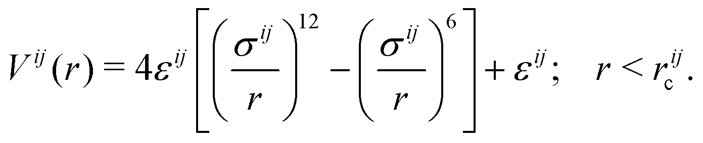 | (1) |
 . rijc = 21/6σij are the cutoff radii of pair interactions. We set εB = 0.1 kcal mol−1, similar to the value of the ionic counterparts εNa = 0.13 kcal mol−1 and εCl = 0.124 kcal mol−1.82–84 The diameter of the polymer beads σB = 0.54 nm is determined by minimising the root-mean-squared error (RMSE) between ρCl and ρClCG (ESI-1, ESI†). The diameters of the CG ions σNa = 0.234 nm and σCl = 0.378 nm are taken from ref. 82 and 84. The PE charge of 35e is neutralized by 35 monovalent counter-anions. In analogy to atomistic-detail simulations, we examine the system response to added monovalent salt concentrations of 0.13 M, 0.26 M, 0.52 M, and 1 M.
The electrostatic interactions were modeled via Coulombic potentials ϕijC. The pairwise interaction between two ionic species i and j with charges ζie and ζje is given by
 | (2) |
It is interesting to note that for the all-atom models there exist innate variations of the dielectric constant between explicit water models such as TIP4P used here. The difference of dielectric constant is due to the choice of the central position of the negative charge in rigid point-charge models,87 but also affected by bond flexibility.88 TIP4P is an extremely versatile water models of this type,89,90i.e. despite some deviation in the value of the dielectric constant as compared to experiments, the overall molecular interactions and the solvation characteristics can be expected to be appropriately reproduced. However, e.g. self-diffusion is influenced.91 We note that any variations in the magnitude of ε between different models will affect the Bjerrum length and rescale the strength of the Coulombic interactions. In the present work such a difference might slightly influence the value of the optimal parameters found for the CG-MD model from the all-atom MD simulations, but this does not affect our results of conclusions.
All CG-MD simulations employ the LAMMPS Jan2020 package.92,93 The long-range electrostatic interactions were calculated using the particle–particle particle–mesh method (PPPM).94 Coulombic pairwise interactions were calculated in real space up to a cut-off of ric = 13σi, where i is any charged species, beyond which the contributions were obtained in reciprocal space. All simulations were performed in the NVT ensemble with a PPPM accuracy of 10−5. The reference temperature was set to 300 K, controlled by the Nose–Hoover thermostat.95,96
Once the initial configuration was prepared, we performed an energy minimization of the system. After this, a 0.2 ns NVT simulation in which the equations of motion were integrated with the velocity Verlet algorithm and 1 fs time step was carried out as initial equilibration of the system. Finally, a 20 ns NVT simulation was run for data analysis, out of which the first 1 ns is disregarded. Here, a 2 fs time step was used.97
In the two-PE case, both PEs are also parallel to the z axis. The first PE is set at the center of the box with (x, y) = (0, 0), while the second PE is set at (x, y) = (d, 0), as shown in Fig. 1(d). With the exception of 70 CG Cl ions for neutralization, all initial settings for the two-PEs case are the same as in the single-PE case.
The equilibration and production run are performed analogous to the single-PE case. For determining the PMF between the two CG PEs, 15 two-PE configurations with PE–PE axial separation distance d between 1 nm and 5 nm at equal intervals were generated. The PEs were kept fixed in position and for each fixed separation distance an MD run of 20 ns was performed. The PMF vs. distance d was calculated by integrating the mean force fCG over the separation distance as  .
.
2.3 Soft-Potential-Enhanced Poisson–Boltzmann theory
Because of its success in describing monovalent ionic environments, the Poisson–Boltzmann (PB) equation is often used to describe the ion distribution and electrostatic potential in electrolyte solutions. The PE is modelled as an impenetrable and rigid cylinder with surface charge density λ/2πa, where a is the cylinder radius. We consider here the case of positively charged PEs which have to be neutralized by adding negative counterions with number density ρci. After this, salt is added to the system. Thus, the number density of cations (ρNa0) equals that of the added salt ρ0. The number density of anions (ρCl0) then equals ρ0 + ρci. The full Poisson–Boltzmann (PB) equation for the electrostatic potential ϕPB(r) surrounding such a cylinder can be written as | (3) |
ρiPB(r) = ρi0![[thin space (1/6-em)]](https://www.rsc.org/images/entities/char_2009.gif) exp(−βeζiϕPB(r)). exp(−βeζiϕPB(r)). | (4) |
In a recent work,53 the prediction of ion number concentration from PB theory was enhanced with a cylindrical soft-potential correction (SPB) of the form
| ρiSPB(r) = ρi0exp(−βζieϕPB(r) − βṼi(r)), | (5) |
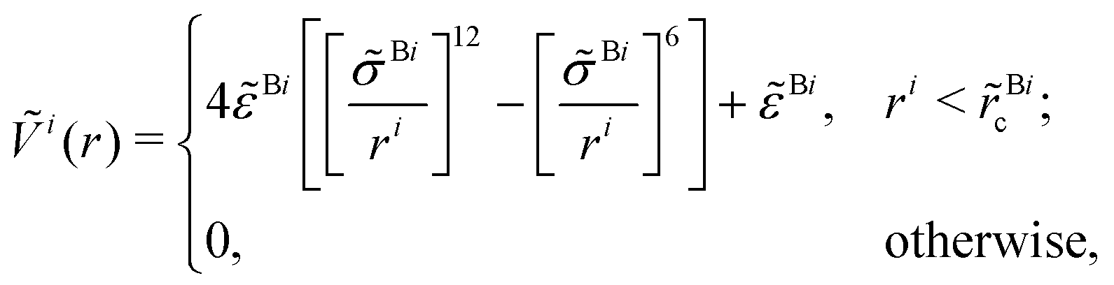 | (6) |
![[r with combining tilde]](https://www.rsc.org/images/entities/i_char_0072_0303.gif) Bic = 21/6
Bic = 21/6![[small sigma, Greek, tilde]](https://www.rsc.org/images/entities/i_char_e10d.gif) Bi. Similar to ref. 53, we use Bi = σBi,
Bi. Similar to ref. 53, we use Bi = σBi, ![[small epsilon, Greek, tilde]](https://www.rsc.org/images/entities/i_char_e0de.gif) BNa = 0.107 kcal mol−1 and BCl = 0.11 kcal mol−1, respectively.
BNa = 0.107 kcal mol−1 and BCl = 0.11 kcal mol−1, respectively.
To obtain accurate results from the SPB theory, the corresponding cylinder radius aSPB has to be adjusted in eqn (5) for the electrostatic potential ϕPB(r). This effective radius may change with system conditions, such as, e.g., ion concentration. The optimization is done by comparing Cl− ion number densities from the CG models with number density of the SPB theory prediction (eqn (5)). From different values of a, eqn (3) allows us to calculate ϕPB(r), followed by eqn (5) to calculate ρClSPB. We identify the optimal radii  giving rise to the optimal potentials
  in eqn (5) based on minimizing the RMSE between ρClCG and ρClSPB. Additional information regarding soft-potential enhanced linear PB (SLPB) theory is provided in ESI-2 (ESI†). The SPB optimized radii (as well as those from SLPB) at different salt concentrations are summarized in Table S1 of the ESI.† It is interesting to note that for different salt concentrations, the radius of the SPB theory only changes marginally (≈±13%). We thus use the average value of
  throughout.
3 Results and discussion
3.1 Single-PE case
We first assess the accuracy of the CG-MD simulations and the SPB and SLPB theories with respect to ion condensation around a single PE. We start by setting up all-atom simulations of a single PDADMA at added monovalent salt concentrations ρ0 = 0.13 M, 0.26 M, 0.52 M and 1.0 M, respectively. To calculate the radially symmetric (perpendicular to the z axis) ion number density profiles ρi(r), the x and y coordinates of the center of mass (CM) of the PE have been taken as the reference point. The density profiles ρNa(r) and ρCl(r) at different salt concentrations are shown in Fig. 2. ρCl obtained from all-atom MD simulations exhibit two peaks at r ≈ 0.45 nm and r ≈ 0.7 nm, respectively. We note that the second peak increases as a function of salt concentration. These peaks are a result of the atomic level structure of PDADMA. Notably, the charged N+ that are usually found at roughly 0.25 nm from the center of the PE are responsible for the enhanced localization of the Cl ions. Details of the atomic configurations are presented in ESI-3 (ESI†). To assess sampling equilibration, the orientational self-correlation function is calculated in ESI-4 (ESI†). | ||
| Fig. 2 The radial number density profiles ρCl(r) and ρNa(r)/ρ0 from all-atom (AA) simulations (large dots), CG model (solid lines), SPB equation (dashed lines) and SLPB equation (dash-dotted lines). The radial number density is calculated in the xy-plane as the function of distance r measured from the PE backbone center axis (all-atom and CG simulations) or the rod center axis (SPB and SLPB models). The insets show details of the data close to the peaks. Here ρ0 = 0.13 M, 0.26 M, 0.52 M and 1.0 M (from left to right). | ||
In the CG model and in SPB theory, we modelled PDADMA as a cylinder with effective radius σBi and  , respectively. These are the only parameters to be optimized, and are obtained by minimizing the RMSE between the different models. Specifically, σBCl = 0.46 nm is obtained from averaging the minimised RMSE between all-atom MD and CG-MD simulations at different added salt concentrations (see the CG-MD simulations part of Methods). On the other hand, the value of
  is obtained by averaging the minimised RMSE between CG-MD simulations and SPB predictions at different added salt concentrations, as reported in the ESI-1 (ESI†). Note that the latter value is also used for SLPB. The comparison between SPB and SLPB theories is shown in ESI-5 (ESI†). In Fig. 2 we report the ion number density profiles from all the different models addressed here. We can see a satisfactory agreement between the different curves, with the exception of the small-scale oscillatory structure in the all-atom MD simulation results, mainly due to local asymmetry of PDADMA which cannot be captured by any of the CG techniques under the current assumptions.
3.2 Two-PE case
In the present case where the system has monovalent ions and is in the weak-coupling regime, there is no charge inversion and the two PDADMA molecules will always repel each other. We quantified the interaction between two PEs via numerical computations of the PMF. Our results from all the different models and different salts here are summarized in Fig. 3, with the all-atom MD being the ultimate benchmark for comparison. The first general observation is that the range of the PMF curves decreases with increasing salt concentration. This is expected and is due to increasing screening effect mediated by the condensing anions. We find good agreement between most of the methods, with the exception of small-amplitude oscillations at d ≈ 1.2 nm that only show up in the all-atom MD data. This feature, as well as the differences rising from the different models, are addressed in more detail in the following sections.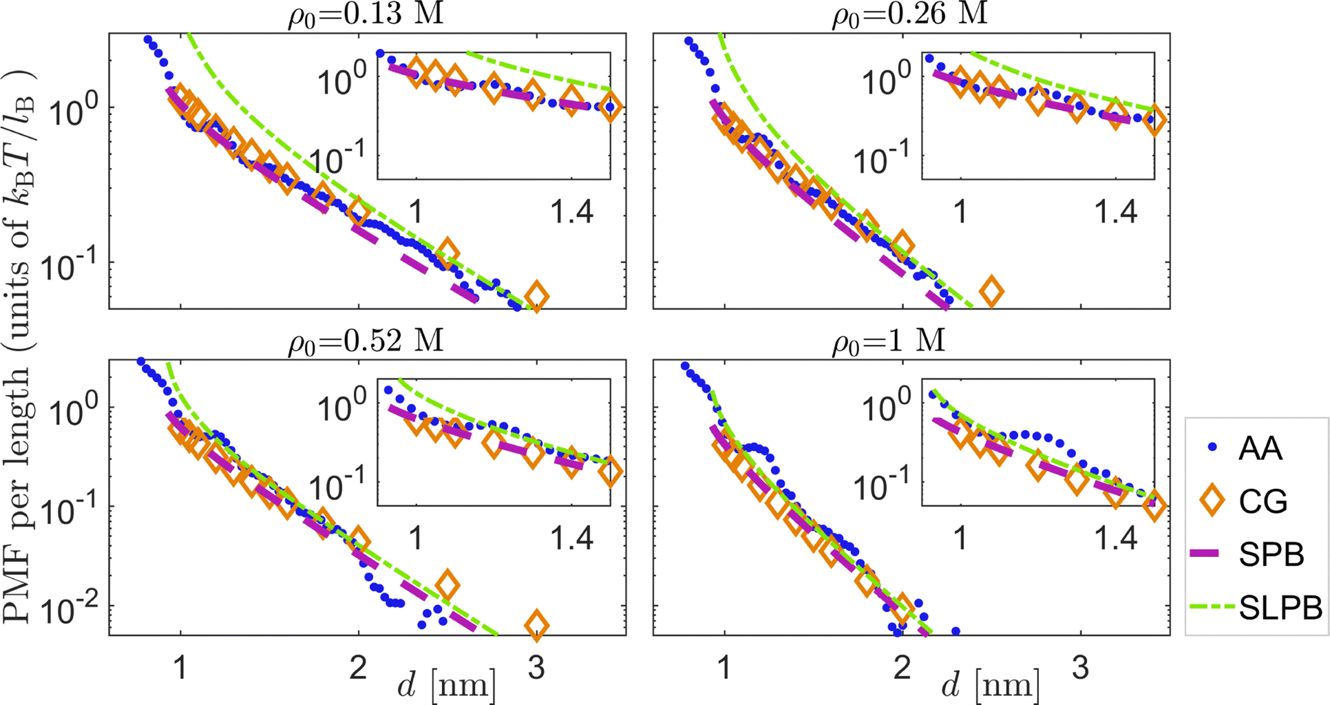 | ||
| Fig. 3 Comparison between the PMFs as a function of distance d obtained from the different models and different salts. The abbreviation AA refers to all-atom MD simulations. The insets show details of the oscillating regions in the PMF profiles. A linear–linear scale version of this figure is shown in ESI-6 (ESI†). | ||
The CG model and SPB theory
In the case of the CG-MD model, the value σB = 0.54 nm is inherited from the single-PDADMA case. The CG model qualitatively captures the PMF curves when benchmarked against all-atom MD simulations at different salt concentrations up to 1 M (see Fig. 3). We find that due to the second PE, the condensation peak maximum of the Cl ions corresponds to 3–4 times higher number density than that of the single PE case at short distances. The detailed results on this are shown in the ESI-7 (ESI†).In order to obtain ϕSPB (abbreviated with ϕ in this section), we employ a finite-element package (COMSOL5.2) to solve eqn (3) in the xy plane with the von Neumann boundary conditions at the surfaces of the two disks, i.e. ∇ϕ·![[n with combining circumflex]](https://www.rsc.org/images/entities/i_char_006e_0302.gif) |x2+y2=a2 = λ/2πaε and ∇ϕ·|(x−d)2+y2=a2 = λ/2πaε. To do so, we use
|x2+y2=a2 = λ/2πaε and ∇ϕ·|(x−d)2+y2=a2 = λ/2πaε. To do so, we use  as obtained in the single-PE case. The same is applied to the SLPB theory. Here is the unit normal vector of each surface, as sketched in Fig. 1(g). The mean electrostatic force between the two cylinders per unit length f(d) at distance d was calculated via the stress integral37
 | (7) |
 is the screening parameter. The mean force can be integrated to get the potential of mean force between two cylinders as
  . We note that the theory could be extended to the case of a non-uniform charge distribution that depends on the vertical coordinate z as λ = λ(z), in which case ϕPB(r) in eqn (3) should be numerically solved under the corresponding boundary conditions. To calculate the mean force f(d) one has to then solve eqn (3.3) in ref. 98.
The SPB prediction of the PMF is in good agreement with the CG model and the all-atom MD simulations, as shown in Fig. 3. In contrast, the PMFs from linear SPB are inaccurate at low salt concentrations. The linear SPB predictions are discussed in more depth in ESI-5 (ESI†).
The influence of the atomistic structure
When the two atomistic detail PDADMA chains in the all-atom MD simulations are separated by a distance comparable to the size of a monomer, the orientations of the PE side chains will affect their interaction. As shown in Fig. 1(e), the 10 charged N+ atoms of each PDADMA chain form in the elongated, axially straight configuration a right-handed cylindrical helix. In cylindrical coordinates, with the longitudinal axis centered at the backbone of each PDADMA chain (see the two black dashed lines in left panel of Fig. 4(a)), the N+ atom of the lth monomer of the kth PE has coordinates (rlk, θlk, zlk), with k = 1, 2 and l = 1, 2,…,10. We take the positive x direction to correspond to θ = 0. We set a plane at z = 0, where the orientations of the two helices are defined by the angles θk (k = 1, 2), respectively, as shown in the right panel of Fig. 4(a). Because the pitch of the helices is Lz/2, the angles θk can be calculated from the location of the first monomer (i.e. l = 1) as θk = θ1k − 4πz1k/Lz. We then define the variable ξ ≡ |θ1 − θ2| to represent the relative orientation between two PDADMA chains. In Fig. 4(b) we show the average value of ξ/π as a function of the distance d between the two PEs. At long distances, the positioning of the PDADMA charges remains uniformly random with 〈ξ〉/π = 1/2. In contrast, at small PE–PE separations of d < 1 nm, the charge group positioning is highly correlated which shows as two orientations coupling strongly. The coupling rises from minimization of electrostatic and steric repulsion by rotation and axial displacement of the PDADMA chains. Nevertheless, the outcome is a strong interchain repulsion evident in the corresponding PMFs. | ||
| Fig. 4 (a) A schematic representation of the charge group positioning in the two PDADMA chains on the left panel; the circles represent charged N+ atoms. A cross-section at the z = 0 plane is shown on the right panel. The orientations of the helices with respect to the positive x direction are defined as θ1 and θ2, and the relative orientation is ξ ≡ |θ1 − θ2|. (b) 〈ξ〉/π as a function of the distance d. The dashed line represents 〈ξ〉/π = 1/2 which corresponds to uncorrelated orientations of the two molecules at long distances (see text for details). | ||
Similar to PDADMA, also DNA exhibits a helical structure of charged atoms, which attract cations in a chemically specific way. In general, some cations are easily absorbed into grooves between two negative phosphate strands, giving rise to opposing stripes with complementary charges along the DNA chain. This configuration creates a “zipper” matching which pulls the parallel molecules together inducing DNA–DNA attraction.99 This attraction contributes to DNA condensation, which has been theoretically addressed in ref. 100 and 101. Furthermore, the response bears strong charge correlations and chemistry specificity. For example, it has been observed that Mn2+ cations are significantly more efficient in condensing DNA than Ca2+ or Mg2+. In fact, Mn2+ is more prone to be absorbed into major grooves to create the “zipper”, while Ca2+ and Mg2+ show a higher affinity to phosphates strands, thus not contributing to DNA condensation.99 However, the contribution rising from this zipper-like attraction cannot be captured by the current form of the SPB theory due to its cylindrical symmetry assumption, charge homogeneity along the PE, and lack of ability to capture the specific charge correlations.
4 Summary and conclusions
In this work we have addressed the interactions between two PEs by using the recently developed soft-potential-enhanced Poisson–Boltzmann (SPB) theory. We have here focused on the case of PDADMA molecules in monovalent salt solutions in the weak-coupling regime, where the interactions are expected to be fully repulsive at all distances. To this end, we have first addressed the ion number density around a single PDADMA. In the elongated, axially straight PE configuration, the charged N+ atoms of PDADMA adopt a helical configuration as their minimum energy configuration by electrostatics and sterics. This leads to the two peaks in the ion distribution around the atomistically detailed PE (see Fig. 2). Although the isotropic SPB theory cannot reproduce such features, it can qualitatively capture the atomistic ion distributions at salt concentrations up to 1 M. By minimizing the RMSE between the number density distribution of the CG model which has been fitted on all-atom MD simulations and the one obtained from SPB theory, we find an optimal effective radius for PDADMA , which is the only (physical) fitting parameter in the SPB theory.
To study the interactions between two PEs we have considered two parallel rodlike PDADMA chains and numerically computed the PMF curves at different salt concentrations. We find that the predictions from the SPB method are accurate when the distance between the two PDADMAs is larger than their radius. There are small oscillations in the PMFs at short distances as revealed by all-atom MD simulations. These oscillations, rising from the chemical structure of the PE, are due to the coupling between charged atoms, steric packing of the side chains, and correlations in the relative orientations of the chains at distances smaller than about 1.3 nm.
At a general level, PE interactions, adsorption and colloidal stability strongly depend on their charge and the added salt.102 Indeed, also PDADMA surface film thickness, uniformity of self-assembling PDADMA film, and more generally the adsorption of PDADMA on substrates have been reported to be highly tunable by added salt.103,104 The present work could provide via interactions mapping easy-to-access guidelines for such tunability, especially with monovalent salts such as KCl in ref. 104. If also oppositely charged PEs were included, extension to PDADMA complexation with oppositely charged PEs, layer-by-layer assembly, and the swelling of the resulting assemblies – all extremely sensitive to added salt105–107 – could be modeled.
While our work suggests that the SPB theory is a simple and accurate way to model interactions in complex PE systems for a large range of system parameters, the limitations of the theory should be kept in mind. We naturally expect the theory to fail when the approximations in the weak-coupling theory are no longer valid. This would happen in cases where the PE line charge density is high, there are electrostatic correlations arising from strong Coulombic interactions, or the assumption of a straightened PE as in our simulation setup leads to a large entropy loss that destabilizes such configurations (see ESI-8 for some additional discussion, ESI†).
Data availability
Link to plotted data is provided at https://doi.org/10.5281/zenodo.6802416. If using the open data, we request acknowledging the authors by a citation to the original source (this paper).Conflicts of interest
There are no conflicts to declare.Acknowledgements
This work was supported by Academy of Finland grant No. 307806 (T. A.-N.) and 309324 (M. S.) and the Academy of Finland Center of Excellence Program (2022–2029) in Life-Inspired Hybrid Materials (LIBER), project number 346111 (M. S.), as well as a Technology Industries of Finland Centennial Foundation TT2020 grant (T. A.-N.). We are grateful for the support by FinnCERES Materials Bioeconomy Ecosystem. Computational resources by CSC IT Centre for Finland and RAMI – RawMatters Finland Infrastructure are also gratefully acknowledged.Notes and references
- J.-L. Barrat and J.-F. Joanny, Adv. Chem. Phys., 1997, 94, 1–66 Search PubMed.
- M. Muthukumar, Macromolecules, 2017, 50, 9528–9560 CrossRef CAS PubMed.
- M. A. C. Stuart, W. T. Huck, J. Genzer, M. Müller, C. Ober, M. Stamm, G. B. Sukhorukov, I. Szleifer, V. V. Tsukruk and M. Urban, et al. , Nat. Mater., 2010, 9, 101–113 CrossRef PubMed.
- C. De las Heras Alarcón, S. Pennadam and C. Alexander, Chem. Soc. Rev., 2005, 34, 276–285 RSC.
- G. Kocak, C. Tuncer and V. Bütün, Polym. Chem., 2017, 8, 144–176 RSC.
- G. C. Wong and L. Pollack, Annu. Rev. Phys. Chem., 2010, 61, 171–189 CrossRef CAS PubMed.
- N. C. Seeman and H. F. Sleiman, Nat. Rev. Mater., 2017, 3, 1–23 Search PubMed.
- Y. Habibi, L. A. Lucia and O. J. Rojas, Chem. Rev., 2010, 110, 3479–3500 CrossRef CAS PubMed.
- M.-C. Li, Q. Wu, R. J. Moon, M. A. Hubbe and M. J. Bortner, Adv. Mater., 2021, 33, 2006052 CrossRef CAS PubMed.
- J. Van der Gucht, E. Spruijt, M. Lemmers and M. A. Cohen Stuart, J. Colloid Interface Sci., 2011, 361, 407–422 CrossRef CAS PubMed.
- S. K. Nemani, R. K. Annavarapu, B. Mohammadian, A. Raiyan, J. Heil, M. A. Haque, A. Abdelaal and H. Sojoudi, Adv. Mater. Interfaces, 2018, 5, 1801247 CrossRef.
- J. X. Tang, S. Wong, P. T. Tran and P. A. Janmey, Ber. Bunseng. Phys. Chem., 1996, 100, 796–806 CrossRef CAS.
- G. B. Sukhorukov, E. Donath, S. Davis, H. Lichtenfeld, F. Caruso, V. I. Popov and H. Möhwald, Polym. Adv. Technol., 1998, 9, 759–767 CrossRef CAS.
- H. I. Ingólfsson, C. A. Lopez, J. J. Uusitalo, D. H. de Jong, S. M. Gopal, X. Periole and S. J. Marrink, Wiley Interdiscip. Rev.: Comput. Mol. Sci., 2014, 4, 225–248 Search PubMed.
- W. G. Noid, J. Chem. Phys., 2013, 139, 090901 CrossRef CAS PubMed.
- G. Lamm, L. Wong and G. R. Pack, Biopolymers, 1994, 34, 227–237 CrossRef CAS PubMed.
- A. Naji and R. R. Netz, Phys. Rev. E, 2006, 73, 056105 CrossRef PubMed.
- M. Deserno, C. Holm and S. May, Macromolecules, 2000, 33, 199–206 CrossRef CAS.
- M. Deserno and C. Holm, Electrostatic effects in soft matter and biophysics, Springer, 2001, vol. 46, pp. 27–50 Search PubMed.
- T. J. Robbins, J. D. Ziebarth and Y. Wang, Biopolymers, 2014, 101, 834–848 CrossRef CAS PubMed.
- P. Batys, S. Luukkonen and M. Sammalkorpi, Phys. Chem. Chem. Phys., 2017, 19, 24583–24593 RSC.
- R. Menes, P. Pincus, R. Pittman and N. Dan, EPL, 1998, 44, 393 CrossRef CAS.
- T. Takahashi, I. Noda and M. Nagasawa, J. Phys. Chem., 1970, 74, 1280–1284 CrossRef CAS.
- J. M. Schurr and B. S. Fujimoto, J. Phys. Chem. B, 2003, 107, 4451–4458 CrossRef CAS.
- Z.-J. Tan and S.-J. Chen, J. Chem. Phys., 2005, 122, 044903 CrossRef PubMed.
- M. Deserno, F. Jiménez-Ángeles, C. Holm and M. Lozada-Cassou, J. Phys. Chem. B, 2001, 105, 10983–10991 CrossRef CAS.
- S. Buyukdagli and T. Ala-Nissila, Langmuir, 2014, 30, 12907–12915 CrossRef CAS PubMed.
- P. Grochowski and J. Trylska, Biopolymers, 2008, 89, 93–113 CrossRef CAS PubMed.
- A. Y. Grosberg, T. Nguyen and B. Shklovskii, Rev. Mod. Phys., 2002, 74, 329 CrossRef CAS.
- I. Borukhov, D. Andelman and H. Orland, Electrochim. Acta, 2000, 46, 221–229 CrossRef CAS.
- S. Lamperski and C. Outhwaite, Langmuir, 2002, 18, 3423–3424 CrossRef CAS.
- B. Tinland, A. Pluen, J. Sturm and G. Weill, Macromolecules, 1997, 30, 5763–5765 CrossRef CAS.
- Y. Lu, B. Weers and N. C. Stellwagen, Biopolymers, 2002, 61, 261–275 CrossRef CAS PubMed.
- H. S. Antila and M. Sammalkorpi, J. Phys. Chem. B, 2014, 118, 3226–3234 CrossRef CAS PubMed.
- H. S. Antila, M. Härkönen and M. Sammalkorpi, Phys. Chem. Chem. Phys., 2015, 17, 5279–5289 RSC.
- J. Heyda and J. Dzubiella, Soft Matter, 2012, 8, 9338–9344 RSC.
- D. Harries, Langmuir, 1998, 14, 3149–3152 CrossRef CAS.
- J. Overbeek, Colloids Surf., 1990, 51, 61–75 CrossRef CAS.
- J.-P. Hsu and B.-T. Liu, J. Colloid Interface Sci., 1999, 217, 219–236 CrossRef CAS PubMed.
- M. K. Gilson, M. E. Davis, B. A. Luty and J. A. McCammon, J. Phys. Chem., 1993, 97, 3591–3600 CrossRef CAS.
- H. Ohshima, Colloid Polym. Sci., 1996, 274, 1176–1182 CrossRef CAS.
- S. L. Brenner and D. A. McQuarrie, J. Colloid Interface Sci., 1973, 44, 298–317 CrossRef CAS.
- S. L. Brenner and V. A. Parsegian, Biophys. J., 1974, 14, 327–334 CrossRef CAS PubMed.
- S. Buyukdagli, Phys. Rev. E, 2017, 95, 022502 CrossRef PubMed.
- S. Buyukdagli and R. Blossey, Phys. Rev. E, 2016, 94, 042502 CrossRef PubMed.
- Y. Levin, Rep. Prog. Phys., 2002, 65, 1577 CrossRef CAS.
- N. Grønbech-Jensen, R. J. Mashl, R. F. Bruinsma and W. M. Gelbart, Phys. Rev. Lett., 1997, 78, 2477 CrossRef.
- J. J. Arenzon, J. F. Stilck and Y. Levin, Eur. Phys. J. B, 1999, 12, 79–82 CrossRef CAS.
- A. Naji, A. Arnold, C. Holm and R. R. Netz, EPL, 2004, 67, 130 CrossRef CAS.
- J. C. Butler, T. Angelini, J. X. Tang and G. C. Wong, Phys. Rev. Lett., 2003, 91, 028301 CrossRef PubMed.
- R. R. Netz and H. Orland, Eur. Phys. J. E: Soft Matter Biol. Phys., 2000, 1, 203–214 CrossRef CAS.
- V. A. Bloomfield, Biopolymers, 1997, 44, 269–282 CrossRef CAS PubMed.
- H. Vahid, A. Scacchi, X. Yang, T. Ala-Nissila and M. Sammalkorpi, J. Chem. Phys., 2022, 156, 214906 CrossRef CAS PubMed.
- C. Wandrey, J. Hernandez-Barajas and D. Hunkeler, Radical Polymerisation Polyeletrolytes, 1999, vol. 145, pp. 123–182 Search PubMed.
- H. H. Strey, R. Podgornik, D. C. Rau and V. A. Parsegian, Curr. Opin. Struct. Biol., 1998, 8, 309–313 CrossRef CAS PubMed.
- Y. Burak, G. Ariel and D. Andelman, Biophys. J., 2003, 85, 2100–2110 CrossRef CAS PubMed.
- J. DeRouchey, R. Netz and J. Radler, Eur. Phys. J. E: Soft Matter Biol. Phys., 2005, 16, 17–28 CrossRef CAS PubMed.
- V. Parsegian, R. Rand and D. Rau, Proc. Natl. Acad. Sci. U. S. A., 2000, 97, 3987–3992 CrossRef CAS PubMed.
- F. Livolant and A. Leforestier, Prog. Polym. Sci., 1996, 21, 1115–1164 CrossRef CAS.
- J. Sitko, E. Mateescu and H. Hansma, Biophys. J., 2003, 84, 419–431 CrossRef CAS PubMed.
- A. B. Harris, R. D. Kamien and T. C. Lubensky, Phys. Rev. Lett., 1997, 78, 1476 CrossRef CAS.
- P. Batys, S. Kivistö, S. M. Lalwani, J. L. Lutkenhaus and M. Sammalkorpi, Soft Matter, 2019, 15, 7823–7831 RSC.
- P. Batys, Y. Zhang, J. L. Lutkenhaus and M. Sammalkorpi, Macromolecules, 2018, 51, 8268–8277 CrossRef CAS PubMed.
- E. Yildirim, Y. Zhang, J. L. Lutkenhaus and M. Sammalkorpi, ACS Macro Lett., 2015, 4, 1017–1021 CrossRef CAS PubMed.
- D. Diddens, J. Baschnagel and A. Johner, ACS Macro Lett., 2019, 8, 123–127 CrossRef CAS PubMed.
- D. Van Der Spoel, E. Lindahl, B. Hess, G. Groenhof, A. E. Mark and H. J. Berendsen, J. Comput. Chem., 2005, 26, 1701–1718 CrossRef CAS PubMed.
- M. J. Abraham, T. Murtola, R. Schulz, S. Páll, J. C. Smith, B. Hess and E. Lindahl, SoftwareX, 2015, 1, 19–25 CrossRef.
- W. L. Jorgensen and J. Tirado-Rives, J. Am. Chem. Soc., 1988, 110, 1657–1666 CrossRef CAS PubMed.
- W. L. Jorgensen and J. D. Madura, Mol. Phys., 1985, 56, 1381–1392 CrossRef CAS.
- J. Aqvist, J. Phys. Chem., 1990, 94, 8021–8024 CrossRef.
- J. Chandrasekhar, D. C. Spellmeyer and W. L. Jorgensen, J. Am. Chem. Soc., 1984, 106, 903–910 CrossRef CAS.
- U. Essmann, L. Perera, M. L. Berkowitz, T. Darden, H. Lee and L. G. Pedersen, J. Chem. Phys., 1995, 103, 8577–8593 CrossRef CAS.
- B. Hess, H. Bekker, H. J. Berendsen and J. G. Fraaije, J. Comput. Chem., 1997, 18, 1463–1472 CrossRef CAS.
- S. Miyamoto and P. A. Kollman, J. Comput. Chem., 1992, 13, 952–962 CrossRef CAS.
- G. Bussi, D. Donadio and M. Parrinello, J. Chem. Phys., 2007, 126, 014101 CrossRef PubMed.
- M. Parrinello and A. Rahman, J. Appl. Phys., 1981, 52, 7182–7190 CrossRef CAS.
- S. Nosé and M. Klein, Mol. Phys., 1983, 50, 1055–1076 CrossRef.
- S. Kumar, J. M. Rosenberg, D. Bouzida, R. H. Swendsen and P. A. Kollman, J. Comput. Chem., 1992, 13, 1011–1021 CrossRef CAS.
- W. Humphrey, A. Dalke and K. Schulten, J. Mol. Graph., 1996, 14, 33–38 CrossRef CAS PubMed.
- L. Martnez, R. Andrade, E. G. Birgin and J. M. Martnez, J. Comput. Chem., 2009, 30, 2157–2164 CrossRef PubMed.
- J. D. Weeks, D. Chandler and H. C. Andersen, J. Chem. Phys., 1971, 54, 5237–5247 CrossRef CAS.
- H. D. Whitley and D. E. Smith, J. Chem. Phys., 2004, 120, 5387–5395 CrossRef CAS PubMed.
- A. A. Siddique, M. K. Dixit and B. L. Tembe, J. Mol. Liq., 2013, 188, 5–12 CrossRef CAS.
- G. S. Freeman, D. M. Hinckley and J. J. de Pablo, J. Chem. Phys., 2011, 135, 10B625 CrossRef PubMed.
- M. Deserno, A. Arnold and C. Holm, Macromolecules, 2003, 36, 249–259 CrossRef CAS.
- W. M. Haynes, D. R. Lide and T. J. Bruno, CRC handbook of chemistry and physics, CRC Press, 2016, vol. 85 Search PubMed.
- M. Neumann, J. Chem. Phys., 1986, 85, 1567–1580 CrossRef CAS.
- G. Raabe and R. J. Sadus, J. Chem. Phys., 2011, 134, 234501 CrossRef PubMed.
- W. L. Jorgensen, J. Chandrasekhar, J. D. Madura, R. W. Impey and M. L. Klein, J. Chem. Phys., 1983, 79, 926–935 CrossRef CAS.
- D. van der Spoel, P. J. Van Maaren and H. J. Berendsen, J. Chem. Phys., 1998, 108, 10220–10230 CrossRef CAS.
- C. J. Fennell, L. Li and K. A. Dill, J. Phys. Chem. B, 2012, 116, 6936–6944 CrossRef CAS PubMed.
- S. Plimpton, J. Comput. Phys., 1995, 117, 1–19 CrossRef CAS.
- A. P. Thompson, H. M. Aktulga, R. Berger, D. S. Bolintineanu, W. M. Brown, P. S. Crozier, P. J. in't Veld, A. Kohlmeyer, S. G. Moore and T. D. Nguyen, et al. , Comput. Phys. Commun., 2022, 271, 108171 CrossRef CAS.
- R. W. Hockney and J. W. Eastwood, Computer simulation using particles, CRC Press, 2021 Search PubMed.
- S. Nosé, Mol. Phys., 1984, 52, 255–268 CrossRef.
- W. G. Hoover, Phys. Rev. A, 1985, 31, 1695 CrossRef PubMed.
- B. Ensing, S. O. Nielsen, P. B. Moore, M. L. Klein and M. Parrinello, J. Chem. Theory Comput., 2007, 3, 1100–1105 CrossRef CAS PubMed.
- N. Hoskin and S. Levine, Philos. Trans. R. Soc., A, 1956, 248, 449–466 CrossRef CAS.
- A. Kornyshev and S. Leikin, J. Chem. Phys., 1997, 107, 3656–3674 CrossRef CAS.
- A. G. Cherstvy, A. A. Kornyshev and S. Leikin, J. Phys. Chem. B, 2002, 106, 13362–13369 CrossRef CAS.
- A. A. Kornyshev and S. Leikin, Proc. Natl. Acad. Sci. U. S. A., 1998, 95, 13579–13584 CrossRef CAS PubMed.
- A. V. Dobrynin and M. Rubinstein, Prog. Polym. Sci., 2005, 30, 1049–1118 CrossRef CAS.
- I. Szilagyi, G. Trefalt, A. Tiraferri, P. Maroni and M. Borkovec, Soft Matter, 2014, 10, 2479–2502 RSC.
- I. Popa, B. P. Cahill, P. Maroni, G. Papastavrou and M. Borkovec, J. Colloid Interface Sci., 2007, 309, 28–35 CrossRef CAS PubMed.
- R. Zhang, Y. Zhang, H. S. Antila, J. L. Lutkenhaus and M. Sammalkorpi, J. Phys. Chem. B, 2017, 121, 322–333 CrossRef CAS PubMed.
- J. T. O’Neal, E. Y. Dai, Y. Zhang, K. B. Clark, K. G. Wilcox, I. M. George, N. E. Ramasamy, D. Enriquez, P. Batys, M. Sammalkorpi and J. L. Lutkenhaus, Langmuir, 2018, 34, 999–1009 CrossRef PubMed.
- E. Guzmán, R. G. Rubio and F. Ortega, Adv. Colloid Interface Sci., 2020, 282, 102197 CrossRef PubMed.
Footnote |
| † Electronic supplementary information (ESI) available. See DOI: https://doi.org/10.1039/d2cp02066a |
| This journal is © the Owner Societies 2022 |