
 Open Access Article
 This Open Access Article is licensed under a
 Creative Commons Attribution 3.0 Unported Licence
First hyperpolarizability of water in bulk liquid phase: long-range electrostatic effects included via the second hyperpolarizability†
Guillaume
Le Breton
 ,
Oriane
Bonhomme
,
Emmanuel
Benichou
and
Claire
Loison
*
,
Oriane
Bonhomme
,
Emmanuel
Benichou
and
Claire
Loison
*
University of Lyon, Université Claude Bernard Lyon 1, CNRS, Institut Lumière Matière, F-69622, Villeurbanne, France. E-mail: claire.loison@univ-lyon1.fr
First published on 25th July 2022
Abstract
The molecular first hyperpolarizability β contributes to second-order optical non-linear signals collected from molecular liquids. For the Second Harmonic Generation (SHG) response, the first hyperpolarizability β(2ω, ω, ω) often depends on the molecular electrostatic environment. This is especially true for water, due to its large second hyperpolarizability γ(2ω, ω, ω,0). In this study we compute the electronic γ(2ω, ω, ω,0) and β(2ω, ω, ω) for water molecules in liquid water using QM/MM calculations. The average value of γ(2ω, ω, ω,0) is smaller than the one for the gaz phase, and its standard deviation among the molecules is relatively small. In addition, we demonstrate that the average bulk second hyperpolarizability 〈γ(2ω, ω, ω,0)〉 can be used to describe the electrostatic effects of the distant neighborhood on the first hyperpolarizability β(2ω, ω, ω). In comparison with more complex schemes to take into account long-range effects, the approximation is simple, and does not require any modifications of the QM/MM implementation. The long-range correction can be added explicitly, using an average value of γ for water in the condensed phase. It can also be easily added implicitly in QM/MM calculations through an additional embedding electric field, without the explicit calculation of γ.
1 Introduction
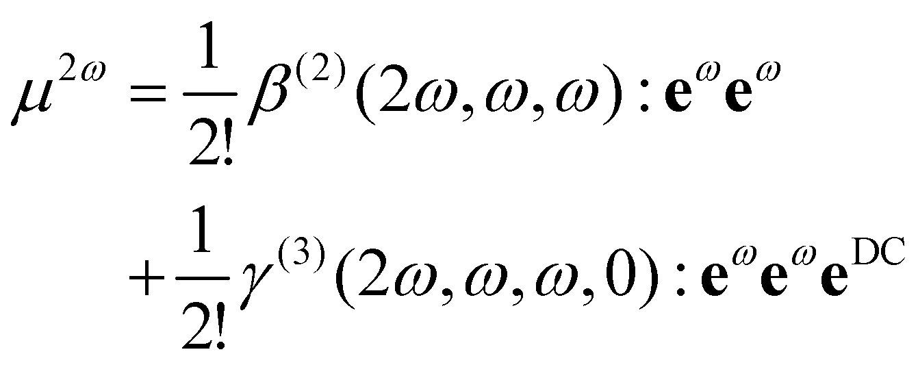
Non-Linear Optical (NLO) technique(s) are increasingly used to probe structural properties of matter. In Second Harmonic Generation (SHG) or Hyper-Rayleigh Scattering (HRS), two photons with the same fundamental frequency interact with a nonlinear material that generates a new photon with twice the energy of the initial photons.1 SHG-based technologies have been developed to investigate simple and complex liquids,2,3 biomimetic systems,4–6 or even biological materials.7,8 One interesting property of non-resonant SHG is the sensitivity of the response to the electrostatic environment.9 Historically, the prototypical application is the electric-field-induced second harmonic generation (EFISHG) of molecules in a gas phase.10 During such experiments, a macroscopic electrostatic field EDC is applied and the SHG response of the system is described using second and third order susceptibility tensor: χ(2)(2ω, ω, ω) and χ(3)(2ω, ω, ω,0), respectively. For a mesoscopic unitary volume, the induced total dipole moment at the second harmonic frequency P2ω expressed as a sum of two terms:| P2ω ∝ χ(2)(2ω, ω, ω): EωEω + χ(3)(2ω, ω, ω,0): EωEωEDC, | (1) |
Eqn (1) was also applied to condensed phases,12,13 and the EFISHG is an established technique to determine the first and the second hyperpolarizabilities of compounds in solutions.14 Even more, studies on liquid/solid or liquid/air interfaces have reported the evolution of the Surface-SHG (S-SHG) response when the surface charge is modulated. Frameworks based on eqn (1) for the fluid nearby the surface have been commonly used in the S-SHG community to extract a surface potential or an effective surface charge.15–19 But the interpretation of the different terms in the S-SHG intensity generated by aqueous solutions is still the subject of many recent works20–23 requiring theoretical calculations at the molecular level.24
To provide an interpretation at the microscopic scale, eqn (1) can also be rewritten at the molecular level:
 | (2) |
The application of field expansions such as eqn (2) for condensed phases is very useful for the interpretation of S-SHG of aqueous solutions, and the values of β and γ for water in liquid water become parameters of the equation. To obtain values of β and γ for water in liquid water, one can use Quantum Mechanical/Molecular Mechanic (QM/MM) calculations.9,24,26,31,32 In such approaches, the electrostatic effect of the environment is included within the QM calculations of a molecular hyperpolarizability βenv for a given electrostatic environment, so that
 | (3) |
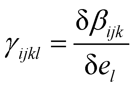 , where βijk (el) is the ijk-component of the first hyperpolarizability of a molecule on which an extra electrostatic field el is applied along the l molecular direction. In the present work, we first provide the βenv and γenv tensors of individual water molecules in the liquid phase using QM/MM approaches at an optical wavelength of 800 nm (typically used for experiments34,35). Relatively to previous works,9,26,32 we detail all the components of both tensors, and discuss the distribution of γ among water molecules.
In a second step, possessing a database of {βenv,γenv} for individual molecules in liquid water, we can additionally scrutinize the validity of the field perturbation approach represented by eqn (2). Similar field expansions for the calculation of solvent effects have been tested for observables such as nuclear magnetic shieldings,36 or linear and non linear optical properties.37 However, the precision of the field expansion for the non-linear optical properties were limited,37 and more terms are needed in the perturbation expression.38 Concerning the first hyperpolarizability of water, Liang et al.9 have compared βenv of water within the liquid phase obtained by QM/MM calculations to the linear field expansion of eqn (2), where eDC was the electrostatic field generated by the surrounding water molecules, noted eenv, and β and γ were the gas-phase values: a quantitative difference emerged. It is therefore expected that the strong solvation of water molecules within liquid water cannot be simplified to eqn (2). Nevertheless, in this work, we show that the perturbation field Taylor expansion can be useful to predict long-range electrostatic effects on the hyperpolarizability of water molecules in their liquid phase.
In the following, Section 2 describes the numerical details. In Section 3, the individual values of γenv and βenv are first reported. Then, we show that the electrostatic field generated by the environment, namely eenv, is strongly heterogeneous in space. Based on this result, we propose to separate the effects of the electric field generated by the environment into a short- and a long-range part. Using this separation, we show that, for a water molecule in the bulk phase, the effect of the long-range electrostatic environment on βenv can be included using a linear correction proportional to γ.
2 Method
The calculations are based on a sequential QM/MM approach in two steps. First, we use a classical Molecular Dynamics (MD) simulation of bulk water to obtain typical structures of the liquid. Then, we compute the first and second hyperpolarizabilities of individual water molecules at the Density Functional Theory (DFT) level, within an electrostatic embedding framework. To investigate fluctuations due to the changing environment, statistics are performed over numerous configurations of the MD simulation.2.1 Molecular dynamics
LAMMPS,39 V.11.08.2017 is used to perform the MD simulation along with the rigid TIP4P/2005 water force field.40 15625 rigid TIP4P/2005 water molecules are placed in a simulation box (approx 7.8 × 7.8 × 7.8 nm3) to form a 3D-periodic bulk system. We have used an isothermal, isobaric ensemble (NPT) with Nose–Hoover thermostat at 300 K (τT = 0.4 ps) and Nose–Hoover barostat at 1 atm (τP = 2 ps).41 1 ns of equilibration is performed before the 1 ns production run, both with a time step of 2 fs. Both electrostatic and Lennard-Jones intermolecular interactions are computed using the long-range Particle-Particle-Particle-Mesh (PPPM) formalism.42,43 Neighbor lists are updated every time step within a radius of 10 Å. This simulation leads to a density of about 0.996 kg L−1. Such a large system was necessary to investigate environmental effects up to 40 Å.2.2 First hyperpolarizability in the liquid phase
To compute the first hyperpolarizability of water molecules within the liquid phase, an explicit environment composed of point charges is used: the Polarizable Embedding model at the zeroth-order (PE0),44,45 implemented in the DALTON software,46 release 2018.2 package. As in our previous recent work,32 the QM calculations were carried out on individual water molecules. Point charges represent the surrounding water molecules, and the same electrostatic description is used as for the MD (TIP4P/2005 model). The MD trajectories are used directly in the QM calculations without further optimization, in contra. We define the parameter Rc as the maximal distance upon which neighbors are included in the PE formalism. The electrostatic field generated by this environment is spatially-heterogeneous in the vicinity of the target molecule and creates a new potential for the target molecule electronic Hamiltonian.The QM/MM approach could be refined by optimizing geometries,47 or by adding dipole, quadrupole or polarizability of the environment,45,48–51 but we shall see in the results that eqn (2) becomes relevant only for long-range effects, where the point-charges electrostatic field is dominant. We have therefore chosen to keep the environment description as simple and robust as possible. To optimize parts of the QM/MM routines, the home-made software FROG is used.‡
The whole procedure is composed of the following steps: (1) perform MD simulation using LAMMPS. (2) Read the MD trajectories using FROG to build the electrostatic environment for each water molecule defined into a sphere of radius Rc centered on the mass center of the target molecule. If a neighbor possesses at least one atom in the sphere, the whole molecule is considered in the environment. The output files for DALTON are created for 300 molecules for 8 selected MD configurations. (3) For each of the 2400 target molecules, calculate the electrostatic field, and its gradients, generated by the environment using FROG. (4) For each of the 2400 target molecules, calculate the value of β at the fundamental wavelength of 800 nm using DFT with the functional CAM-B3LYP52 and the basis d-aug-cc-pVTZ,53 using the quadratic response formalism as implemented in DALTON.54 (5) Read all DALTON output files and analyze the data using FROG.
The largest inaccuracy of our approach is due to the QM method and the corresponding functional. For the first hyperpolarizability of water molecules, the values in vacuum obtained with our method (DFT/CAM-B3LYP) are typically overestimated by about 10%32 in comparison to the golden standard for QM/MM calculation of small molecules (CCSD55–57). Both calculation schemes use the TIP4P/2005 rigid force field, the MM size Rc = 15 Å and the basis is d-aug-pVTZ. The basis set d-aug-cc-pVTZ53 used is widespread across the community26,55–57 and presents a good balance between accuracy and cost. In a previous work,32 we have observed a smooth convergence of the first hyperpolarizability relative to the basis-set size for water in bulk water, and similar absolute values of the nuclear and electronic contributions to the electrostatic and polarization energies. Therefore, we estimate that spill-out effects are not dominant,50 even if we use the large d-aug-cc-pVTZ basis set. We have not taken into account the nuclear degree of freedom (vibrational effects) since Beaujean et al.58 have shown that this effect is small for the second hyperpolarizability of water, especially at small wavelengths.
2.3 Second hyperpolarizability in the liquid phase
In this work, we are interested in the evolution of the first hyperpolarizability under a static and homogeneous electrostatic field, which is reflected by γ(2ω, ω, ω, 0) noted here γ. For each individual molecule, the second hyperpolarizability γ can be computed from the first hyperpolarizability β using the Finite Field (FF) framework. For that, we use the PE formalism described above to compute β when an extra homogeneous electrostatic field is applied, and then compute γ according to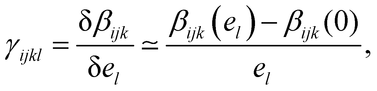 | (4) |
| ijkl | Vacuum | Liquid | ||
|---|---|---|---|---|
| γ vac | 〈γenv〉 | σ[γenv] | ||
| aaaa | 1110 | 740 | 140 |
|
| bbbb | 4090 | 2940 | 650 | |
| cccc | 2000 | 1400 | 230 | |
| aabb | 930 | 640 | 200 | |
| bbaa | 1060 | 710 | 150 | |
| baab | 1010 | 680 | 220 | |
| abba | 940 | 660 | 140 | |
| aacc | 590 | 370 | 60 | |
| ccaa | 610 | 380 | 80 | |
| caac | 610 | 380 | 60 | |
| acca | 590 | 370 | 80 | |
| bbcc | 1120 | 770 | 170 | |
| ccbb | 1010 | 720 | 180 | |
| cbbc | 1010 | 730 | 150 | |
| bccb | 1060 | 750 | 200 | |
Frequency dispersion can be important for γ: for example, Beaujean et.al.58 have shown a variation of about 25% between an excitation wavelength of 800 nm and at the infinite wavelength limit for γ(3ω, ω, ω, ω). Here, even if we are using a Finite Field approach, the frequency dispersion of β related to the fundamental frequency (here 800 nm) is correctly reproduced since we use the first hyperpolarizability obtained using the frequency dependent response scheme.
2.4 Embedding environment size: Rc
One of the objectives of this study is to understand the impact of the electrostatic environment on the first hyperpolarizability, distinguishing the effects of close and far neighbors. Therefore, different values of Rc are used for β calculations. In the following, the notation βPE (Rc) denotes the hyperpolarizability obtained by a QM/MM calculation at a given Rc and e(Rc) the electric field generated by this PE environment. In this notation, Rc = 0 corresponds to a gas phase calculation. According to previous works,32,57,59 a large environment (typically between 10 and 20 Å) is necessary to obtain a good convergence of the β values. Here, for each molecule, a reference calculation is performed using the PE formalism with an extremely large radius of Rf = 40 Å, and we consider that βenv = βPE (40 Å). Similarly, we consider that the electrostatic field eenv = e (40 Å). Note that such a large radius still does not represent the complete MD liquid phase, described using periodic boundary conditions.On the contrary, the variation of γ with the size of the environment is not investigated in details here. Therefore, the PE radius used to compute the second hyperpolarizability γ is set to 10 Å. Yet, we have verified that the γ does not evolve much using larger radius in agreement with Osted et al.59 (data not shown) and have noted it γenv.
2.5 Statistical averaging
The first and second hyperpolarizability in the liquid phase are obtained from 2400 configurations of the PE environment. These configurations are extracted from 8 MD snapshots, with 300 water molecules randomly selected in each frame. These frames are separated by 100 ps to ensure time decorrelation.32 We have verified that this number of configurations is sufficient to reach convergence; indeed, the numerical error due to the configuration number is about 1% (see ESI,† Fig. S2 and S3). This is smaller than the error due to the DFT Finite field calculation relative to CCSD calculations (see ESI,† Tables S2 and S3). The C2v symmetry of the first and second hyperpolarizability obtained by QM/MM confirms this good convergence (see the Section 3 and ESI,† Section S2.1).3 Results
In the following, Section 3.1 first presents the second hyperpolarizability tensor γ calculated using QM/MM approaches for single water molecules within the liquid bulk phase, and the standard deviation of the calculated values. Then, Section 3.2.1 presents some difficulties encountered when applying eqn (2) for condensed phases. We attribute them to the properties of the electrostatic field generated by the environment, eenv, described in 3.2.2. Based on these results, and on eqn (2), in Section 3.2.3, we propose a correction to β that permits to include long-range interactions. Finally, we show that this correction enhances the precision of standard QM/MM calculations.3.1 QM/MM results: second hyperpolarizability of water in the bulk phase
Table 1 presents the values of selected γ components calculated either in the vacuum or in liquid phase – the other non-zero components of γ are presented in ESI,† Table S4.For the vacuum phase, the molecular C2v symmetry is fulfilled: the only non-vanishing components are the γiiii and γiijj for i and j in {a, b, c}, plus their permuted terms1 (see ESI,† Table S4). In the liquid phase, this symmetry is not valid for individual values, but is recovered for the average 〈γenv〉. Our results agree with the ones by Osted et al.59 within about 15%. We impute the discrepancies to both the difference of methods (DFT vs. CCSD, different MD models) and the difference of excitation wavelengths (800 vs. 1080 nm). More detailed comparisons with literature are provided in ESI,† Section S1.1.
Noticeably, when transferred into the laboratory frame, the average second hyperpolarizability becomes centro-symmetric (see ESI,† Table S5), indicating that our sampling of molecular orientation in the liquid phase is sufficient. Interestingly, the average value of all C2v-authorized γenv components are positive. Moreover, in the liquid phase, the γenv components are about 30% smaller than the ones in the vacuum – see ESI,† Fig. S4.
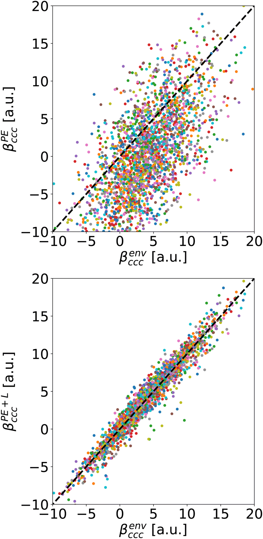
Beyond the average values, the environment induces fluctuations of γenv, and of βenv. A typical and relevant case is illustrated by Fig. 1, displaying the join probabilities of {βccc,γcccc} obtained for the 2400 water molecules within their environment. Projections on the axes display the distributions of βccc and γcccc separately. As already discussed in the literature,32,57,59 the water first hyperpolarizability fluctuations in the liquid phase are strong, with standard deviations similar to the absolute values of the averages – for instance 〈βenvccc〉 = 4.1 a.u. and σ [βenvccc] = 3.1 a.u. For individual molecules, some β components, null in average, can be larger than the one with a net average (see ESI,† Fig. S4).
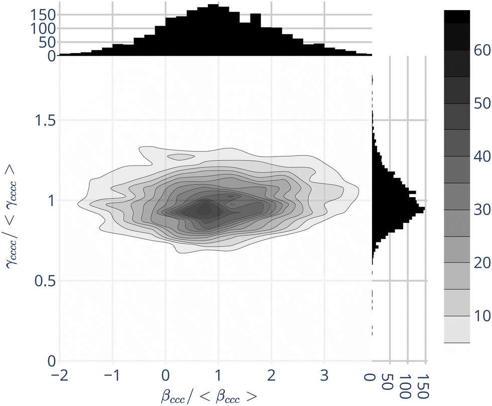 | ||
| Fig. 1 Join population of {βenvccc,γenvcccc} obtained by QM/MM approaches for bulk liquid water. The independent ones are presented on the top and right for the βenvccc and γenvcccc respectively. The values are normalized with respect to their average ones:〈 βenvccc〉 = 4.1 a.u. and 〈γenvcccc〉 = 1400 a.u. | ||
In complement to the results published by Osted et al.,59 we show that the second hyperpolarizability γ also fluctuates, but in a smaller extent than β: the standard deviations of the different components σ [γenv] are about 20% of their average values 〈γenv〉 – see Fig. 1 for γcccc, and ESI,† Table S4.
Fig. 1 moreover shows that the values of β and γ are not strongly correlated. Hence, in the following, we neglect the γenv dispersion and attribute the same second hyperpolarizability 〈γenv〉 to all the water molecules.
3.2 Using γ to calculate individual β in condensed phases
After describing the second hyperpolarizability γenv in the liquid phase, we will question if it can be used to predict the first hyperpolarizability of water molecules in the liquid phase using different approximations inspired by eqn (2). We shall compare the βenv obtained by QM/MM to linear expansions relative to a perturbing electric field.| βGR = βvac + γ0·eenv, | (5) |
If the linear proportionality factor γ0 is known, and the same for all molecules, this approach would be very helpful: the liquid first hyperpolarizability depends only on eenv. An MD simulation can provide eenv for each molecule, and the liquid phase first hyperpolarizability is calculated using eqn (5), so that no expensive QM/MM approach is needed. Moreover, such an approximation is commonly used in the Surface-SHG community (for example ref. 18 and 19).
Liang et al.57 have reported that eqn (5) using the vacuum value for the second hyperpolarizability γ0 = γvac is a poor estimator for βenv. We have thus applied eqn (5) using the average bulk second hyperpolarizability tensor γ0 = 〈γenv〉 for all the molecules (values from Table 1 and from ESI,† Table S4), and the electrostatic field generated by the environment eenv. For liquid water, the distribution of the largest component of eenv, along the water molecular axis c is represented on Fig. 2: it has typical values around 3 × 10⁻² a.u., i.e. 1.6 V Å−1. The other components average to zero, with approximately the same standard deviations (data not shown).
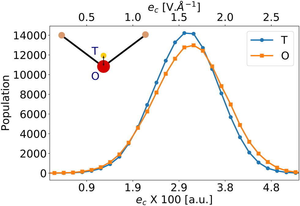 | ||
| Fig. 2 Distribution of the electrostatic field generated by the environment eenv along the molecular c-axis. The electrostatic field is measured at 2 positions: at the oxygen atom position (O: orange squares), or at the negative charge one (T: blue dots) according to the TIP4P/2005 force field. The O and T positions are distant by 0.15 Å. | ||
The predicted average values 〈βGR〉 are compared to the QM/MM values 〈βenv〉 in Table 2. First, the addition of the linear correction in eqn (5) allows recovering signs for βGR components in agreement with βenv. However, the βGR model largely over-estimates the reference values: the correction γ0·eenv should be smaller. This overshooting is even worse when the vacuum value γvac is used for γ0, as Liang et al. had tested.9 Thus, even if it contains some relevant physics, eqn (5) describing a correction that is proportional to eenv is not workable: it predicts an average hyperpolarizability 〈βGR〉 one order of magnitude too large.
| ijk | 〈βvac〉 | 〈βenv〉 | 〈βGR〉 |
|---|---|---|---|
| ccc | −15.3 | 4.1 | 28.5 |
| caa | −12.5 | −2.0 | −0.6 |
| aca | −12.4 | −2.0 | −0.8 |
| cbb | −5.0 | 2.5 | 17.7 |
| bcb | −7.4 | 2.2 | 16.9 |
Moreover, the value of eenv in eqn (5) is ill-defined because of its strong spatial heterogeneity. To highlight this fact, Fig. 2 presents the electrostatic field created by the environment along the molecular c-direction, eenvc, calculated at 2 positions within the embedded molecule: either at the position of the negative charge of the TIP4P/2005 model, or at the position of the oxygen atom. While the 2 distributions look very similar, a difference on the average values of about 10−3 a.u. appears. Given the large value of γcccc (≈1400 a.u., see Table 1), the component βccc predicted by βGR changes by about 40%, depending on where eenv is calculated. Therefore, we attribute the failures of eqn (5) to the strong intensity and large gradient of the embedding field eenv, which are incompatible with a simple linear expansion. Such limitations of perturbation field expansions to model solvation effects had already been discussed in the literature. When studying the nuclear magnetic shielding tensors of the atoms of N-methylacetamide solvated by liquid water, Kjaer et al.36 have shown that the field experienced by the nuclei is very inhomogeneous, so that considering one averaged field from all configurations and/or across all nuclei is not a good approximation.
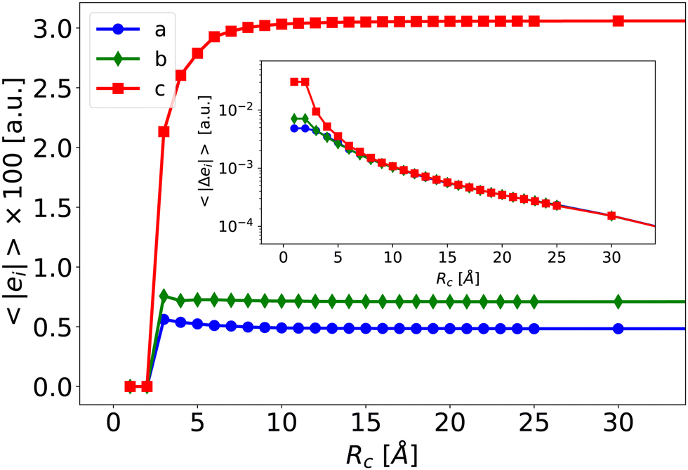 | ||
| Fig. 3 Averaged norm of the electrostatic field generated by the electrostatic environment (e(Rc)) felt at the T-position, for increasing environment size Rc. In insert, the difference Δe(Rc) relative to the value at Rc = 40 Å, in logarithmic scale as a function of the size Rc. | ||
Given that the closest shells are responsible for both the intensity and the heterogeneity of eenv, we divide the neighborhood into two parts, as illustrated on Fig. 4.
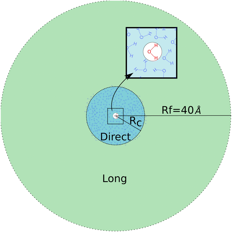 | ||
| Fig. 4 Sketch of the electrostatic embedding procedure. The QM box is defined for only one molecule of water at the center. Direct area, until Rc: all the neighbors are included in a QM/MM calculation with discrete solvation procedure, such as the PE formalism. Long-range area, from Rc to Rf: the neighbors are included by the electrostatic field they generate at one specific point of the QM box. | ||
The direct area contains the closest neighbors of the target molecule (at the center), up to a distance Rc: they create a strong and heterogeneous electric field, noted e(Rc). The long-range area, due to neighbors beyond Rc from the target molecules, creates a less intense and more homogeneous electric field on the target molecule.
The total embedding electrostatic field eenv is thus separated into a short-range contribution e(Rc), and a correction, Δe(Rc) due to the long-range electrostatic interactions:
| eenv = e(Rc) + Δe(Rc). | (6) |
 (see ESI,† Fig. S1). Generally, the corrections to the gradients are small (typically 10−4 a.u) for neighbors further away than 10 Å. Since the correction Δe(Rc) is more homogeneous than eenv, it hardly depends on the point on which it is calculated. In the following, we use the value of Δe(Rc) evaluated at the T-position.
For the first hyperpolarizability, as for eenv, we describe the impact of the environment in two different ways depending on the neighbors distance. The direct neighbors within the sphere of radius Rc are included explicitly in the QM/MM calculation through the PE approach. The long-range neighbors, beyond Rc, are included implicitly via the homogeneous field they produce on the target molecule, Δe(Rc), with a correction proportional to 〈γenv〉. This approximation can be viewed as a linear expansion relative to the value of first hyperpolarizability already perturbed by the direct neighbors, βPE(Rc):
| βPE+L(Rc) = βPE(Rc) + 〈γenv〉·Δe(Rc). | (7) |
In the following, we compare this approximation of β, noted βPE+L(Rc) and the usual QM/MM calculation where only the PE scheme up to a distance Rc is used, noted βPE(Rc). To estimate the accuracy of the two approximations PE and PE + L as a function of Rc, we compare them to our reference values βenv.
As a typical example, we compare on Fig. 5 the βccc computed with Rc = 5 Å either using PE approximation (top) or the PE + L one (bottom) to the reference value βenvccc. The diagonal dashed lines represent the case where the approximation reproduces exactly the reference.
 | ||
| Fig. 5 Comparison of the reference individual molecular βenvccc component and the one obtained using PE (TOP) and PE + L (BOTTOM) approximation with Rc = 5 Å. The dashed line corresponds to the ideal case where a correction matches perfectly the expected value. Each dot represents a molecule. | ||
For the usual calculation (βPE), there is a systematic error leading to inaccuracy: at Rc = 5 Å, the average value of βPEccc is smaller than the one of βenvccc. Moreover, the error fluctuates a lot, it can reach tens of a.u., depending on the molecule. On the contrary, the PE + L approach almost quantitatively reproduces the reference, even for Rc as small as 5 Å
To illustrate the effect of Rc, Fig. 6 depicts the evolution of 〈βPE〉 and 〈βPE+L〉 as a function of Rc for the ccc component (similar trends are obtained for other components). As expected, the inaccuracy of the PE and PE + L approaches decreases when Rc increases.
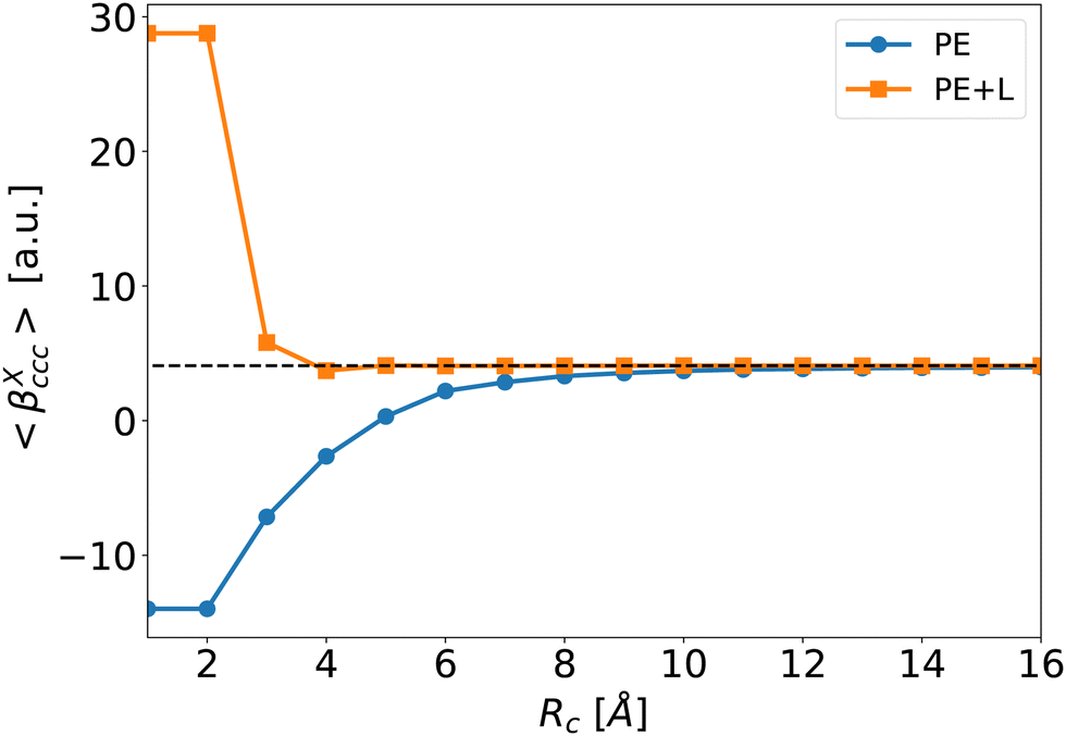 | ||
| Fig. 6 Average of the βXccc (Rc) component as a function of Rc for the PE (blue disks) and PE + L (orange squares, see eqn (5)) approximations. The dashed line is the reference value βenv obtained for Rf = 40 Å. | ||
When the correction is added, the convergence is reached faster (Rc = 4 Å) compared to the usual βPE calculation (Rc ≃ 12 Å). The effect of the neighbors further than 5 Å can thus be very efficiently included by a second hyperpolarizability corrective term. Beyond the description of the average first hyperpolarizability, Fig. 5 also illustrates that the PE + L approach improves the precision of the individual predictions. This can be quantified through the mean absolute error (MAE), averaged over all the N = 2400 molecular configurations and all the 27 components, noted ΔβT:
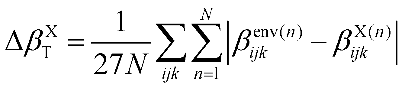 | (8) |
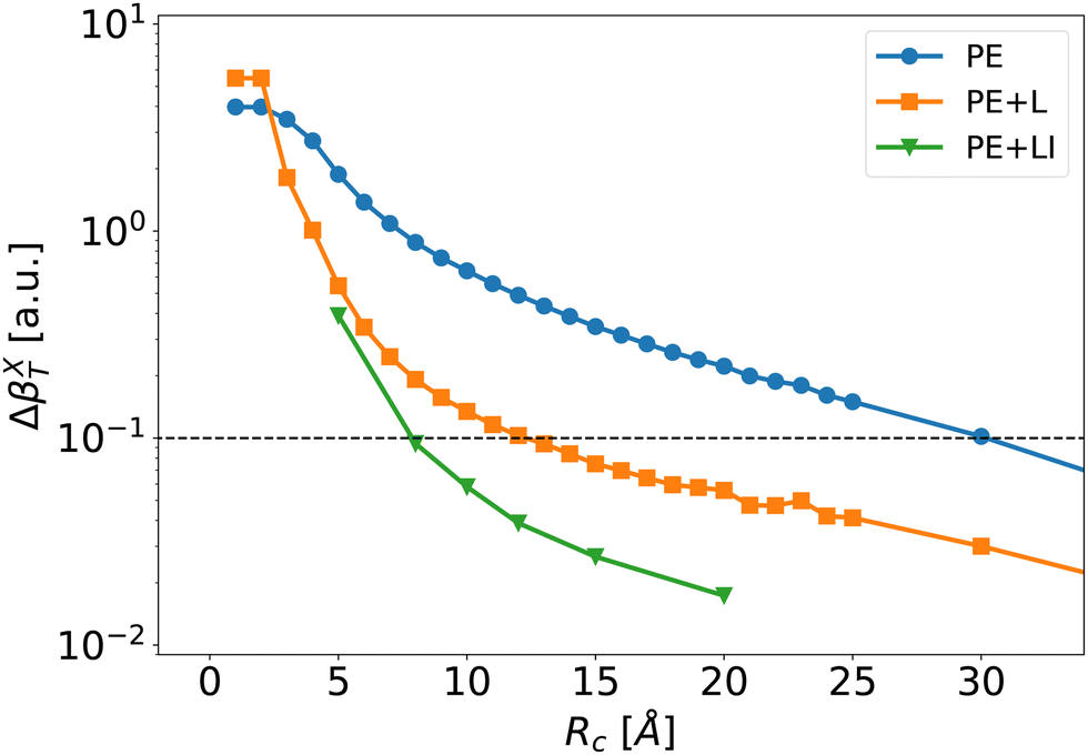 | ||
| Fig. 7 Mean absolute error of the individual first hyperpolarizability tensor defined by eqn (8) as a function of Rc for the PE (blue disks), PE + L (orange squares) and PE + LI (green triangles) approximations. The dashed line corresponds to an error of 0.1 a.u. at which we define convergence. | ||
The long-range correction provides very good results and reaches an error below 0.1 a.u. at Rc = 12 Å. To obtain the same degree of accuracy, one would need to include explicitly neighbors up to Rc ≃ 30 Å in the usual PE scheme without long-range correction. For Rc larger than 10 Å, the error obtained with the long range correction (PE + L) is about one order of magnitude lower than the one with the traditional PE approach. This shows that – once the strong short-range effects are explicitly included – it is possible to use the knowledge of γ to predict accurately the long-range electrostatic effects on β. Note that the long-range correction is proportional to the average value 〈γenv〉, i.e.Eqn (9) neglects γenv fluctuations. As discussed further in ESI,† Section S4, including the fluctuations of γenv in eqn (9) only slightly improves the results. However, it implies to compute γenv for every molecule, which greatly increases the numerical cost. Therefore, using an average γenv is a very good compromise between computational cost and accuracy, at least for bulk liquid water.
| βPE+LI (Rc) = βPE (Rc; e(Rc)). | (9) |
Fig. 7 illustrates that the PE + LI values of the first hyperpolarizability are very close to the reference values. The PE + LI approach is even more precise that the PE + L because (1) the second hyperpolarizability fluctuations are neglected in PE + L – not in PE + LI, and (2) the second hyperpolarizability is calculated with finite field approach in PE + L – not in PE + LI. The PE + LI correction does not require the knowledge of the second hyperpolarizability. It can be seen as a simplification of more elaborated QM/MM developments taking into account long-range environment in non-periodic QM/MM methods.60–63 Indeed, long-range effects can be approximated by boundary potential models, by cutoff method coupled with switching and shifting functions, by the so-called Long-Range Electrostatic Correction, or by additional charges on the edge of the MM embedding, or in the MM embedding. Our simpler approach with a homogeneous electrostatic field is intended to provide the impact of the remote MM environment on the non-linear optical property of the QM system. It is limited to sequential QM/MM approaches where the trajectory is obtained independently. The advantages of the PE + LI are (1) its insight in the physical origin of the correction and its link with usual equations used in the experimentalist community, and (2) its simplicity and low computational cost. Finally, the value of e(Rc) could include periodic boundary conditions, but it is beyond the present work.
4 Conclusions
In this work, we have computed the first and second hyperpolarizability of water in the liquid phase using state-of-the-art QM/MM calculations. With this set of values, several approaches were tested to take into account the electrostatic environment in the first hyperpolarizability.The second hyperpolarizability is high in the bulk phase. The neighborhood induces a dispersion on the second hyperpolarizability γ(2ω, ω, ω,0) values, but less than for the first hyperpolarizability.
Concerning the first hyperpolarizability β, linear expansions are valid for a weak and spatially-homogeneous electrostatic field, while the embedding electrostatic field created by the liquid surroundings is not. To compute individual molecular hyperpolarizability in the liquid phase, the molecular structure of the nearest neighbors have to be described explicitly, and QM/MM models are very relevant.
But long-range effects, up to several nanometers, can become heavy to take into account using QM/MM approaches, since a very large number of neighbors have to be included. This problem is expected to become all the more pregnant when the environment is anisotropic, with charges or polarization. We have proposed to consider the effect of long-range electrostatic environment on the liquid first hyperpolarizability using the average second hyperpolarizability γ. This long-term correction increases the precision of the hyperpolarizability calculation, and speeds up the convergence of the average value relative to the QM/MM environment size Rc. For pure bulk water, our approximation makes sense for a long-range part defined beyond 5 to 10 Å, depending on the quantity required. From a numerical point of view, the correction can be powerful for charged environments because the size of the explicit embedding region can be reduced drastically.
This work has demonstrated the promising potentialities of using the second hyperpolarizability, explicitely or implicitely to predict first hyperpolarizabilities. The present study is applied to pure water bulk phase at 300 K. However, the correction developed here should be also relevant for many other system geometries or compositions, where the long-range electrostatic effects can modify optical responses. If necessary, an extension including electric field gradients would also be straightforward using the Dalton package. Precision tests remain to be performed for more complex systems such as salted aqueous solutions, or charged interfaces.
Author contributions
GLB: conceptualization, methodology, validation, writing. OB: supervision, validation, writing. EB: supervision, writing, review, editing. CL: supervision, validation, writing.Conflicts of interest
There are no conflicts to declare.Acknowledgements
We thank P.-F. Brevet for insightful discussions. We gratefully acknowledge support from the PSMN (Pôle Scientifique de Modélisation Numérique) of the ENS de Lyon for the computing resources.Notes and references
- P.-F. Brevet, Surface Second Harmonic Generation, 1997.
- M. C. Goh, J. M. Hicks, K. Kemnitz, G. R. Pinto, K. Bhattacharyya, K. B. Eisenthal and T. F. Heinz, J. Phys. Chem., 1988, 92, 5074–5075 CrossRef CAS.
- Q. Wei, D. Zhou and H. Bian, Phys. Chem. Chem. Phys., 2018, 20, 11758–11767 RSC.
- M. N. Nasir, E. Benichou, C. Loison, I. Russier-Antoine, F. Besson and P.-F. Brevet, Phys. Chem. Chem. Phys., 2013, 15, 19919–19924 RSC.
- G. Licari, J. S. Beckwith, S. Soleimanpour, S. Matile and E. Vauthey, Phys. Chem. Chem. Phys., 2018, 20, 9328–9336 RSC.
- E. Donohue, S. Khorsand, G. Mercado, K. M. Varney, P. T. Wilder, W. Yu, A. D. MacKerell, P. Alexander, Q. N. Van, B. Moree, A. G. Stephen, D. J. Weber, J. Salafsky and F. McCormick, Proc. Natl. Acad. Sci. U. S. A., 2019, 116, 17290–17297 CrossRef CAS PubMed.
- M. E. Didier, O. B. Tarun, P. Jourdain, P. Magistretti and S. Roke, Nat. Commun., 2018, 9, 1–7 CrossRef PubMed.
- S. Bancelin, C. Aimé, I. Gusachenko, L. Kowalczuk, G. Latour, T. Coradin and M. C. Schanne-Klein, Nat. Commun., 2014, 5, 1–8 Search PubMed.
- C. Liang, G. Tocci, D. M. Wilkins, A. Grisafi, S. Roke and M. Ceriotti, Phys. Rev. B, 2017, 96, 1–6 Search PubMed.
- P. Kaatz, E. A. Donley and D. P. Shelton, J. Chem. Phys., 1998, 108, 849–856 CrossRef CAS.
- J. Yang, E. V. Barnat, S.-k Im and D. B. Go, J. Phys. D: Appl. Phys., 2022, 55(22), 225203 CrossRef.
- B. Levine and C. Bethea, J. Chem. Phys., 1976, 65, 2429–2438 CrossRef CAS.
- T. N. Ramos, S. Canuto and B. Champagne, J. Chem. Inf. Model., 2020, 60, 4817–4826 CrossRef CAS PubMed.
- B. F. Levine and C. G. Bethea, J. Chem. Phys., 1975, 63, 2666–2682 CrossRef CAS.
- E. C. Yan, Y. Liu and K. B. Eisenthal, J. Phys. Chem. B, 1998, 102, 6331–6336 CrossRef CAS.
- T. Joutsuka, T. Hirano, M. Sprik and A. Morita, Phys. Chem. Chem. Phys., 2018, 20, 3040–3053 RSC.
- S. Pezzotti, D. R. Galimberti, Y. R. Shen and M.-P. Gaigeot, Phys. Chem. Chem. Phys., 2018, 20, 5190–5199 RSC.
- L. Dalstein, K.-Y. Chiang and Y.-C. Wen, J. Phys. Chem. Lett., 2019, 10, 5200–5205 CrossRef CAS PubMed.
- A. Marchioro, M. Bischoff, C. Lütgebaucks, D. Biriukov, M. Předota and S. Roke, J. Phys. Chem. C, 2019, 123, 20393–20404 CrossRef CAS PubMed.
- R. Hartkamp, A. L. Biance, L. Fu, J. F. Dufrêche, O. Bonhomme and L. Joly, Curr. Opin. Colloid Interface Sci., 2018, 37, 101–114 CrossRef CAS.
- L. B. Dreier, C. Bernhard, G. Gonella, E. H. Backus and M. Bonn, J. Phys. Chem. Lett., 2018, 9, 5685–5691 CrossRef CAS PubMed.
- E. Ma, P. E. Ohno, J. Kim, Y. Liu, E. H. Lozier, T. F. Miller, H.-F. Wang and F. M. Geiger, J. Phys. Chem. Lett., 2021, 12, 5649–5659 CrossRef CAS PubMed.
- H. Chang, P. E. Ohno, Y. Liu, E. H. Lozier, N. Dalchand and F. M. Geiger, J. Phys. Chem. B, 2020, 124, 641–649 CrossRef CAS PubMed.
- Y. Foucaud, B. Siboulet, M. Duvail, A. Jonchere, O. Diat, R. Vuilleumier and J.-F. Dufrêche, Chem. Sci., 2021, 12, 15134–15142 RSC.
- G. Maroulis, Chem. Phys. Lett., 1998, 289, 403–411 CrossRef CAS.
- J. Kongsted, A. Osted, K. V. Mikkelsen and O. Christiansen, J. Chem. Phys., 2004, 120, 3787–3798 CrossRef CAS PubMed.
- M. Hidalgo Cardenuto and B. Champagne, Phys. Chem. Chem. Phys., 2015, 17, 23634–23642 RSC.
- T. Giovannini, M. Ambrosetti and C. Cappelli, Theor. Chem. Acc., 2018, 137(6), 74 Search PubMed.
- P. Beaujean and B. Champagne, J. Chem. Phys., 2019, 151, 064303 CrossRef.
- T. N. Ramos, F. Castet and B. Champagne, J. Phys. Chem. B, 2021, 125, 3386–3397 CrossRef CAS PubMed.
- L. Jensen and P. T. Van Duijnen, J. Chem. Phys., 2005, 123(7), 074307 CrossRef PubMed.
- G. Le Breton, O. Bonhomme, P.-F. Brevet, E. Benichou and C. Loison, Phys. Chem. Chem. Phys., 2021, 23, 24932–24941 RSC.
- A. Willetts, J. E. Rice, D. M. Burland and D. P. Shelton, J. Chem. Phys., 1992, 97, 7590–7599 CrossRef CAS.
- O. Bonhomme, L. Sanchez, E. Benichou and P. Brevet, J. Phys. Chem. B, 2021, 125, 10876–10881 CrossRef CAS PubMed.
- A. Pardon, O. Bonhomme, C. Gaillard, P.-F. Brevet and E. Benichou, J. Mol. Liq., 2021, 322, 114976 CrossRef CAS.
- H. Kjaer, S. P. A. Sauer and J. Kongsted, J. Chem. Phys., 2011, 134, 44514 CrossRef PubMed.
- Y. Luo, P. Norman, I. Introduction and H. Agren, J. Chem. Phys., 1998, 109, 3589–3595 CrossRef CAS.
- K. O. Sylvester-Hvid, K. V. Mikkelsen, P. Norman, D. Jonsson and H. Ågren, J. Phys. Chem. A, 2004, 108, 8961–8965 CrossRef CAS.
- S. Plimpton, J. Comput. Phys., 1995, 117, 1–19 CrossRef CAS.
- J. L. Abascal and C. Vega, J. Chem. Phys., 2005, 123, 234505 CrossRef CAS PubMed.
- G. J. Martyna, D. J. Tobias and M. L. Klein, J. Chem. Phys., 1994, 101, 4177–4189 CrossRef CAS.
- R. E. Isele-Holder, W. Mitchell and A. E. Ismail, J. Chem. Phys., 2012, 137 Search PubMed.
- R. E. Isele-Holder, W. Mitchell, J. R. Hammond, A. Kohlmeyer and A. E. Ismail, J. Chem. Theory Comput., 2013, 9, 5412–5420 CrossRef CAS PubMed.
- J. M. H. Olsen and J. Kongsted, Advances in Quantum Chemistry, Academic Press, 2011, vol. 61, pp. 107–143 Search PubMed.
- E. R. Kjellgren, J. M. Haugaard Olsen and J. Kongsted, J. Chem. Theory Comput., 2018, 14, 4309–4319 CrossRef CAS PubMed.
- K. Aidas, C. Angeli, K. L. Bak, V. Bakken, R. Bast, L. Boman, O. Christiansen, R. Cimiraglia, S. Coriani and P. Dahle, et al. , Wiley Interdiscip. Rev.: Comput. Mol. Sci., 2014, 4, 269–284 CAS.
- H. C. Georg and S. Canuto, J. Phys. Chem. B, 2012, 116, 11247–11254 CrossRef CAS PubMed.
- N. H. List, H. J. A. Jensen and J. Kongsted, Phys. Chem. Chem. Phys., 2016, 18, 10070–10080 RSC.
- M. T. Beerepoot, A. H. Steindal, N. H. List, J. Kongsted and J. M. H. Olsen, J. Chem. Theory Comput., 2016, 12, 1684–1695 CrossRef CAS PubMed.
- C. Steinmann, P. Reinholdt, M. S. Nørby, J. Kongsted and J. M. H. Olsen, Int. J. Quantum Chem., 2019, 119, e25717 CrossRef.
- A. Marefat Khah, P. Reinholdt, J. M. H. Olsen, J. Kongsted and C. Hattig, J. Chem. Theory Comput., 2020, 16, 1373–1381 CrossRef CAS PubMed.
- T. Yanai, D. P. Tew and N. C. Handy, Chem. Phys. Lett., 2008, 393, 51–57 CrossRef.
- R. A. Kendall, T. H. Dunning and R. J. Harrison, J. Chem. Phys., 1992, 96, 6796–6806 CrossRef CAS.
- P. Sałek, O. Vahtras, T. Helgaker and H. Ågren, J. Chem. Phys., 2002, 117, 9630–9645 CrossRef.
- P. Besalú-Sala, S. P. Sitkiewicz, P. Salvador, E. Matito and J. M. Luis, Phys. Chem. Chem. Phys., 2020, 22, 11871–11880 RSC.
- P. Beaujean and B. Champagne, Theor. Chem. Acc., 2018, 137, 50 Search PubMed.
- C. Liang, G. Tocci, D. M. Wilkins, A. Grisafi, S. Roke and M. Ceriotti, Phys. Rev. B, 2017, 96, 1–6 Search PubMed.
- P. Beaujean and B. Champagne, J. Chem. Phys., 2019, 151, 064303 CrossRef.
- A. Osted, J. Kongsted, K. V. Mikkelsen, P. O. Åstrand and O. Christiansen, J. Chem. Phys., 2006, 124, 124503 CrossRef PubMed.
- G. A. Cisneros, M. Karttunen, P. Ren and C. Sagui, Chem. Rev., 2014, 114, 779–814 CrossRef CAS PubMed.
- T. Vasilevskaya and W. Thiel, J. Chem. Theory Comput., 2016, 12, 3561–3570 CrossRef CAS PubMed.
- X. Pan, K. Nam, E. Epifanovsky, A. C. Simmonett, E. Rosta and Y. Shao, J. Chem. Phys., 2021, 154, 024115 CrossRef CAS PubMed.
- J. Nochebuena, S. Naseem-Khan and G. A. Cisneros, Wiley Interdiscip. Rev.: Comput. Mol. Sci., 2021, 11, e1515 CAS.
Footnotes |
| † Electronic supplementary information (ESI) available: Methodological details; symmetry, averages and standard deviations of water second hyperpolarizability in the liquid phase; heterogeneity of the electrostatic field generated by the neighborhood; impact of second hyperpolarizability fluctuations on the γ long correction. See DOI: https://doi.org/10.1039/d2cp00803c |
| ‡ This code is deposited on Zenodo platform https://doi.org/10.5281/zenodo.5998193, and available on demand to the authors. |
| This journal is © the Owner Societies 2022 |