Martini 3 coarse-grained force field for poly(para-phenylene ethynylene)s

Abstract

Poly(para-phenylene ethynylene)s, or short PPEs, are a class of conjugated and semi-flexible polymers with a strongly delocalized π electron system and increased chain stiffness. Due to this, PPEs have a wide range of technological applications. Although the material properties of single-chains or mixtures of few PPE chains have been studied in detail, the properties of large assemblies remain to be fully explored. Here, we developed a coarse-grained model for PPEs with the Martini 3 force field to enable computational studies of PPEs in large-scale assembly. We used an optimization geometrical approach to take the shape of the π conjugated backbone into account and also applied an additional angular potential to tune the mechanical bending stiffness of the polymer. Our Martini 3 model reproduces key structural and thermodynamic observables of single PPE chains and mixtures, such as persistence length, density, packing and stacking. We show that chain entanglement increases with the expense of nematic ordering with growing PPE chain length. With the Martini 3 PPE model at hand, we are now able to cover large spatio-temporal scales and thereby to uncover key aspects for the structural organization of PPE bulk systems. The model is also predicted to be of high applicability to investigate out-of-equilibrium behavior of PPEs under mechanical force.

---

1 Introduction

Poly(para-phenylene ethynylene)s, or short PPEs, are a class of conjugated and semi-conductive polymers with a strong delocalized π electron system extending over the entire backbone.^1,2 Due to the π conjugation of the carbon atoms, PPEs exhibit unique optical and optoelectronic properties,^3–6 and therefore have a wide range of applications, ranging from the printing of electronic devices (e.g. organic transistors, organic light emitting diodes, and organic photovoltaic cells) to the fabrication of biological and chemical sensors.^7–11 The backbone of PPEs is composed of aromatic rings and stiff triple bonds, which are linked by single carbon bonds (Fig. 1). Based on the alternation of single and multiple bonds, the orbitals of the carbon atoms overlap and the π electrons are delocalized from one end of the polymer to the other. The delocalization of the π electrons is the reason for the planar structure of monomers and the linear backbone together with its increased mechanical bending stiffness.¹² Therefore, PPEs can be classified as semi-flexible polymers and the bending stiffness can be characterized by the persistence length of a single polymer.¹³ Previous studies determined the persistence length of PPEs through a combination of light scattering experiments or electron paramagnetic resonance spectroscopy and computational methods. Cotts et al. obtained a persistence length of 13.5–16 nm and Godt et al. obtained an estimate of 14.3–19.1 nm.^14,15 PPEs thus are roughly 10 to 50-fold stiffer than most polymers with non-conjugated backbones, such as polyethylene (0.45 ± 0.1 nm)^16,17 or polymethyl methacrylate (1.2 ± 0.1 nm),^18,19 a feature that could be exploited in the development of composite materials with tunable elasticity resulting in unique mechanical properties.^20,21

Fig. 1 Chemical structure of the poly(para-phenylene ethynylene)s. The polymer backbone consists of alternating phenylene rings and a stiff triple bond linked by single bonds. For the side-chains we assume R = H.

Computational simulation is a reliable technique to determine the material properties of conjugated polymers, such as PPEs.^22,23 The molecular origin of the high stiffness has been addressed with high-level-of-accuracy quantum mechanical calculations. In fact, both the excited states and the energy barrier of the torsion angle for the backbone rotation of di(para-phenylene ethynylene)s or bis(phenyl ethynyl) benzenes were determined using density functional theory (DFT) simulations.^23,24 Bagheri et al. combined molecular dynamics (MD) with DFT simulations to improve the Optimized Potential for Liquid Simulation (OPLS) force field to ensure the planarity of the PPE backbone.^12,23 Several studies performed all-atom (AA) MD simulations, using this developed OPLS force field, to simulate the conformation of single PPE chains to thereby examine the rigidity and side-chain aggregation in different solvents.^12,25,26 However, DFT calculations and AA-MD simulations are limited to small PPE systems, since both are computationally costly and sample the conformational space inefficiently.²⁷ Alternatively, coarse-grained MD is a well-established approach to cover larger spatio-temporal scales compared to AA-MD by reducing the atomistic degrees of freedom.²⁸ Godt et al. developed a simplified freely rotating chain model for PPE backbones by substituting the phenylene ring, the bond between the phenylene and ethynylene unit and the triple bond with one single bead each.¹⁵ Although this model reproduces the global stiff nature of PPEs, it lacks the chemical and thermodynamic distinction between aromatic rings and triple bonds giving rise to the π stacking. Hence, there exists no CG model that considers atomistic structure on the one hand and enables the simulation of large semi-flexible PPE networks on long timescales, capturing their thermodynamic behavior appropriately, on the other hand.

To address this question, we developed a CG model for PPEs based on the Martini 3 force field.²⁹ The Martini force field is one of the most commonly applied CG models in the field of biomolecules or materials science.^30–33 Martini 3 is based on reparameterised small and tiny beads with improved solute–solvent interactions to better reproduce stacking properties, like the bulk density and the oil–water partitioning behavior.³⁴ The force field offers the advantage of capturing larger spatio-temporal scales of molecular systems while adjusting the level of resolution of their molecular components. In particular, Martini 3 is very suitable to model long PPE chains, and even mixtures of them, while still taking the essential chemical details of the aromatic rings and the triple bond, giving rise to the enhanced chain stiffness, into account. In detail, the Martini force field is based on a building block principle.³⁵ Each building block is parameterised separately to cover a diverse spectrum of chemical moieties.³⁶ The parameterisation of the building blocks relies on reproducing experimentally determined thermodynamic properties, like the partitioning free energies of a broad range of chemical substances between polar and apolar solvents.³⁷ Besides this top–down approach, the parameterisation of the bonded interactions relies on a bottom–up method through the use of AA simulations.³⁸ For PPEs, we used a geometrical model to consider the shape of the conjugated backbone and an additional harmonic bond angle potential to fine-tune its mechanical bending stiffness. We analyzed the structural organization within the bulk material by characterizing the nematic alignment of PPEs. We find that the degree of alignment decreases with increasing chain length, showing how the dynamics of long-chain semi-flexible PPEs is increasingly driven by entropic effects. Hence, our Martini 3 PPE model adequately reproduces the transition from the rigid rod to random coil like behavior of semi-flexible polymers. It thus enables the study of large bulk systems of such polymers close to atomistic resolution, and together with backmapping and multi-scale approaches allows characterization of the intriguing structural, mechanical and electronic properties of this remarkable material.

2 Methods

For Martini 3, on average, four heavy atoms plus the associated hydrogens are replaced by one CG interaction site.²⁷ To take more complex structures into account (e.g. especially aromatic rings as in the case of PPE), higher resolution mapping is recommended, where three or two heavy atoms plus the associated hydrogens are substituted by one small or tiny bead.^28,34 For PPEs, we followed the standardized bottom-up top-down Martini philosophy and defined four tiny beads as our main building block (Fig. 2A). Next, we compared the octanol-/water partitioning free energy of di(para-phenylene ethynylene) to experimental measurements reported in the literature to select the respective bead type of each building block.^39,40 For the optimization of bonded interactions, we used a bottom-up strategy by matching the probability densities, describing the bonded potentials, from CG to AA reference simulations.²⁹ We performed all simulations, both Martini 3 and AA, with the GROMACS 2020 molecular dynamics simulations package.⁴¹ A detailed protocol regarding the setup of each simulation is described in the following sections.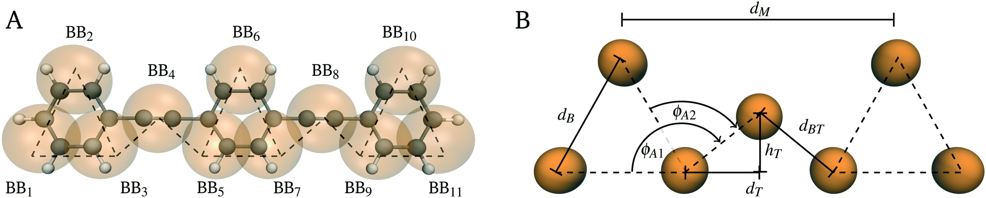

Fig. 2 Mapping scheme and geometrical modeling. (A) Mapping from AA (black) to CG (orange) resolution. The dotted lines represent the bonded potentials of the CG model. (B) The geometrical model takes the shape of the PPE backbone into account. PPEs are represented as a linear chain of regular triangles with side length d_B and spacing d_M. The remaining equilibrium values are calculated by trigonometrical relations (eqn (8)–(10)).

2.1 All-atom simulation protocol

For the AA simulations of PPEs we used a modified version of the OPLS force field. The modification is implemented by converting parameters from the Polymer Consistent Force Field to OPLS and applying a Rickaert–Bellemanns torsion potential to keep the backbone of the polymer planar.²³ Bagheri et al. performed DFT simulations to determine an energetic barrier of 4 kJ mol⁻¹ for the rotation of phenylene units, slightly above the experimental values of approximately 2 to 2.5 kJ mol⁻¹ from fluorescence spectroscopy.^42–44 The setup of the AA force field for PPEs is described in more detail by Bagheri et al.^12,23

2.1.1 All-atom single and multiple chains. As a reference system for the parametrization of the CG model, we selected one single chain of PPE, consisting of four monomers, solvated with the SPC2016 water model in a cubic simulation box. We performed an energy minimization using the steepest descent algorithm by gradually switching off the restraints along the backbone.⁴⁵ Next, we increased the temperature of the system to 300 K by operating the velocity rescaling thermostat for 500 ps with a relaxation timestep of τ_T = 0.1 ps.⁴⁶ For the NPT equilibration, we stabilized the pressure at 1 bar using the Parinello–Rahman barostat for 500 ps with τ_P = 2 ps and a compressibility of 4.5 × 10⁻⁴ bar⁻¹.⁴⁷ During the equilibration steps, we applied the Verlet-scheme to cut off the short-range electrostatics and van der Waals interactions at 1.0 nm.⁴⁸ The long-range electrostatic interactions were treated with the Particle-Mesh-Ewald scheme.^49,50 We simulated the solvated PPE chain for 100 ns. For simulations of multiple chains, we randomly distributed ten single chains of the same length in a simulation system of 10 × 10 × 10 nm³, and solvated the chains in water. We then used the same setup described above for a single chain and performed a 100 ns production run to monitor the chain packing within the polymer bundle.

2.1.2 All-atom bulk system. To setup the bulk system for the packing analysis of PPEs, we first applied the GROMACS gmx insert-molecules command to randomly insert 300 chains, consisting of four monomers each, into a box of 80 × 80 × 80 nm³. Next, we energy minimized the system in three steps and applied the stochastic dynamics integrator to perform a NVT equilibration for 1 ns at 300 K with τ_T = 0.1 ps.⁵¹ We gradually reduced the box volume for 100 ns to give the chains enough time to assemble into a dense structure and used the Parinello–Rahman barostat with τ_P = 2 ps and a 1 fs timestep to equilibrate the system and prevent numerical instabilities.⁵² Finally, we performed a 1 μs production run to allow the alignment of PPEs to form an equilibrated bulk system.

2.2 Coarse-grained simulation protocol

To develop a CG model of PPEs, we chose the Martini 3 force field.²⁹ We used the Martini PolyPly package to generate the topology and coordinate files for PPEs with a different polymerization degree.³⁶ We applied the common Martini 3 MD simulation parameters to calculate the neighbor list and to consider the electrostatics or van der Waals interactions.²⁹ The Verlet neighbor search algorithm updated the neighbor list every 20 to 40 steps with a buffer tolerance of 0.005 kJ mol⁻¹ ps⁻¹. For electrostatics, the reaction-field cut off the coulomb potential at r_c = 1.1 nm with a relative permittivity of ε_r = 15. We modeled the van der Waals interactions with the Lennard-Jones potential, a cutoff at r_c = 1.1 nm and the potential-shift with the Verlet scheme.^33,53 If not stated otherwise, we selected the common Martini 3 MD parameter set from the Martini webportal (https://www.cgmartini.nl)⁵⁴ for the equilibration and production run simulations.^29,34,55

2.2.1 Coarse-grained single and multiple chains. The parameterisation of the bonded potentials between the CG beads was derived from a single chain in solution simulation. We used the steepest descent algorithm to energy minimize one single chain of four monomers in a vacuum, which we then solvated in a cubic box with Martini 3 water beads and a van der Waals radius of 0.21 nm as well as a box with toluene.⁵⁶ The solvated system was energy minimized, while restraining the positions of the polymer backbone. For the constant temperature, volume and particle number ensemble, the velocity rescaling thermostat increased the temperature to 300 K for 5 ns with a time constant of τ_T = 1.0 ps. Next, we equilibrated the system in the NPT ensemble applying the Parinello–Rahman barostat to stabilize the pressure at 1 bar with τ_P = 12 ps and a compressibility of 3 × 10⁻⁴ bar⁻¹. Subsequently, we performed a production run for 100 ns with a 20 fs timestep for both the single chain in solution and the assembly of ten chains in the solution setup.

2.2.2 Coarse-grained bulk system. The bulk system for the Martini 3 model consisted of hundreds of PPE chains of varying polymer length. To get the initial positions of the chains, we applied the GROMACS gmx insert-molecules command to randomly insert between 300 and 800 PPEs, each with a chain length of 20, 40 and 60 repetition units, in a large 1000 × 1000 × 1000 nm³ box of vacuum. For the energy minimization of the bulk system, we applied the steepest descent algorithm. Next, we used the stochastic dynamics integrator to ensure a stochastic temperature coupling during the equilibration steps. The stochastic integrator stabilized the temperature for 5–8 ns at 300 K with a relaxation timestep of τ_T = 1.0 ps. Subsequently, we decreased the box volume for 1 μs to give the PPE chains sufficient time to assemble into a network structure. To this end, we deformed the simulation box constantly with a deformation velocity of −1.2 to −0.8 m s⁻¹ and a reduced timestep of 5 fs to ensure numerical stability. Starting from the deformed bulk system, we applied the Parinello–Rahman barostat with τ_P = 12 ps and a reduced timestep of 2 fs to stabilize the pressure at 1 bar for 2–10 ns to prevent numerical instabilities. At the end, we performed a 5 microseconds production run with at least a 20 fs timestep to sample the free energy landscape of the bulk system sufficiently. In addition, we performed simulated annealing simulations,⁵⁷ based on the Martini setup for polymers,^58,59 to sample energetically favourable states of the PPE networks. For this purpose, we increased the temperature to 400 K for 20 ns, 500 K for 20 ns, 600 K for 160 ns and finally to 800 K for 1.8 microseconds using a 10 fs timestep. Next, we cooled down the system to 300 K during a 400 ns equilibration giving the polymer chains sufficient time to self-organize. In comparison with experimental annealing cycles at ∼360 K, we annealed on a shorter timescale at higher temperatures.⁶⁰

2.3 Free energy calculations

The partitioning free energy of tolane, short for di(para-phenylene ethynylene), in an octanol-/water system forms the basis for selecting the Martini 3 bead types. We performed umbrella sampling of tolane in an octanol-/water simulation box to determine the free energy of transfer together with the potential of mean forces and the partition coefficient. The partition coefficient describes the distribution of solute between two immiscible solvents and can be compared to experiments.⁶¹ For the umbrella sampling, we defined a reaction coordinate pointing from the center of the hydrophilic solvent towards the center of the hydrophobic one with a 0.05 nm window spacing. Next, we restrained the solute for 100 ps with a force constant of 1000 kJ mol⁻¹ nm⁻², energy minimized each window with the steepest descent algorithm and equilibrated the system for 3 ns with a 10 fs timestep. We applied the velocity rescaling thermostat to stabilize the temperature at 300 K with τ_T = 1 ps and the Parrinello–Rahman barostat to keep the pressure at 1 bar with τ_P = 12 ps and a compressibility of 3 × 10⁻⁴ bar⁻¹. To ensure appropriate sampling of the free energy landscape, we simulated each window for 500 ns with a 25 fs timestep. We applied the weighted histogram analysis method,⁶² as implemented in gmx wham,⁶³ to estimate the potential of mean forces (PMF) and derive the partition coefficient:⁶¹where logP_Oct−H2O is the partition coefficient for tolane in an octanol-/water system, ΔG_i describes the free energy for tolane in solvent i, T is the temperature and R is the universal gas constant. In addition, we checked for PMF convergence⁶⁴ by backward block averaging the free energy barrier for tolane in the biphasic octanol-/water system using a 5 ns step size and performed a Bayesian bootstrap analysis to quantify the statistical uncertainty of the free energy estimates.⁶³

2.4 Methods for validation

The validation of the developed CG model followed a mixed bottom–up top–down strategy by comparing the properties of interest with experimental data or AA simulations. In particular, we focused on reproducing the mechanical bending stiffness of the polymer by identifying the persistence length, and on its packing properties, by calculating the bulk density and the orientation of packed chains. For this purpose, we imported the trajectory into Python using the Molecular Dynamics Analysis software package (MDAnalysis) and determined the properties with the Numerical Python package (NumPy).^65–67 In the case of the packing analysis, we not only calculated the orthogonal distances between aligned chains, but also projected the center-of-mass of each polymer onto the main center-of-mass (COM) axis of the polymer bundle.

2.4.1 Persistence length. The persistence length describes the intrinsic bending stiffness of the polymer chain, thereby characterizing its local flexibility.^68,69 The persistence length L_P is defined from the gradient of the exponentially declining orientation correlations of the unit tangent vector along the backbone of the polymer chain:⁷⁰

〈cos ϕ_ij〉 = 〈t⃑_j·t⃑_i〉/〈L_M²〉 = exp(−N_M〈L_M〉/L_P) (2)

Here, t⃑_i and t⃑_j are the unit tangent vectors of segment i or j, respectively; ϕ_ij is the angle spanned between t⃑_i and t⃑_j; N_M is the number segments between i and j, and 〈L_M〉 is the average length of one segment. To get an estimate for the persistence length, we loaded the CG trajectory into Python and applied the scalar product function of NumPy to determine the angle between each pair of segments along the backbone ϕ_ij. More specifically, we defined the CG beads representing the triple bonds as the segments of the polymer chain, linked adjacent segments by a vector, and then normalized each vector to obtain the unit tangent vector. Hence, we received a chain of unit tangent vectors following the backbone of the polymer. From this chain, we calculated the pair-wise scalar product t⃑_i, t⃑_j to estimate the cosines of the angles ϕ_ij enclosed by two segments i and j. Next, we averaged the cosines of the angles over the number of segments N_M = |j − i| before averaging over time. We also applied the worm-like chain theory to estimate the persistence length.⁷¹ For this purpose, as proposed by Doi et al., the square of the orientation correlations (eqn (2)) was integrated along the curvature of the chain,⁷²where 〈R_e²〉 is the mean squared end-to-end distance of the polymer to be determined from CG simulations. For this calculation, we used the trajectory from the single chain in solution protocol to calculate the end-to-end distance between each pair of segments along the polymer chain with NumPy. Subsequently, we squared and averaged the end-to-end distances over the count of chain segments N_M, before averaging over time, as described above. After preparing the CG data, we plotted both the averaged cosine angles 〈cos ϕ_ij〉 and squared end-to-end distances 〈R_e²〉 as a function of the count of segments N_M. To estimate the persistence length of semi-flexible PPEs, we fitted eqn (2) and (3) to the trajectory obtained from CG simulations using the curve fitting function from the Scientific Python package.⁷³

2.4.2 Packing properties. The packing of the CG model is characterized by the assembly of multiple PPEs into a parallelly aligned bundle. We analyzed the packing of the Martini 3 model by comparing the axial and radial displacement of single chains within the bundle to experiments and AA simulations. For the radial displacement, we estimated the π stacking by calculating the orthogonal distance between chains of the bundle. For the axial displacement, we determined the main COM axis of the bundle, and projected the COM of each polymer onto the main COM axis. To estimate the orthogonal distance between adjacent polymers d_π, we defined the end-to-end vector for a single chain of the bundle R⃑_e, and linked the COM of all the other polymers to one end of the end-to-end vector R⃑_p. From the norm of the vector product between R⃑_e and R⃑_p, we computed the area content spanned by both vectors and divided the normalized vector product by the length of the end-to-end vector |R⃑_e| to estimate the orthogonal distances between adjacent polymer chains:

In addition, we determined the axial displacement describing the movement of parallelly aligned polymers. We estimated the axial displacement of chains by projecting the COM for each polymer orthogonally onto the main COM axis of the bundle. More precisely, we defined the main COM axis as the vector between the COMs at both ends of the bundle R⃑_b, linked one end of the COM axis to the COM of any other polymer R⃑_k and projected the COM of each polymer onto the main COM axis, according to⁷⁴

Here, P⃑_Rb(R_k) denotes the vector projection of the COM of the polymer onto the COM axis of the bundle. We normalized the projected vector |P⃑_Rb(R_k)| and subtracted half the length of the main COM axis |R⃑_b| to obtain the axial displacement for the COM of each polymer with regard to the COM of the bundle. In the end, we used the kernel density estimator from the Seaborn package to compute the respective probability density.⁷⁵

2.4.3 Density of the bulk system. For the analysis of the bulk system, we focused on both macroscopic and microscopic properties that characterize the packing of multiple PPEs within a polymer network. On the macroscopic scale, we estimated the bulk density of PPEs from both AA and CG simulations by performing a NPT equilibration and computing the property of interest from the resulting energy file with the gmx energy command. In addition, we rescaled the Martini 3 density with the ratio of molar masses from the AA and CG representation to enable the comparison with AA simulations.

2.4.4 Radial distribution function. On the microscopic scale, we analyzed the spatial correlation by computing the radial distribution function (RDF). To allow a detailed evaluation of Martini 3 simulations with respect to the AA ones, we first mapped both the AA and CG trajectory to the same one-bead-per aromatic ring resolution. Next, we imported the mapped trajectory into MDAnalysis, excluded the intrachain beads and used the InterRDF command to compute the RDF between N_P polymers consisting of N_M beads each. The RDF g_ij(r) quantifies the probability of finding bead i from polymer I at a distance r from bead j belonging to polymer J > I:⁷⁶where r⃑_i and r⃑_j denote the position vectors of bead i and j from polymer I and J and with i ∈ I and j ∈ J, respectively; r is the distance from a reference bead i; δ corresponds to the Dirac delta function and g₀ = 4ρπr²dr represents a factor used to normalize the RDF with respect to a uniform system.

2.4.5 Nematic correlation function. Besides the pair-wise spatial correlation, we estimated the nematic correlation function (NCF) to characterize the orientation of different polymer chains relative to each other.⁷⁷ The NCF Π_ij(r) quantifies the alignment of different PPE chains within the bundled network by combining the orientation correlations with the RDF. The NCF weights the probability of finding two beads i and j at a distance r = |r⃑_i − r⃑_j| with the absolute value of the dot product of their tangent vectors t⃑_i and t⃑_j, as defined in eqn (7):As before, i and j denote the beads of polymer I and J. Hence, the NCF describes the decay of orientation correlations with increasing distance between beads. We notice that the upper and lower limit of eqn (7) is given as a step function with height one for parallelly aligned and one half for randomly oriented chains.⁷⁷ To estimate the NCF, we extended the InterRDF command by multiplying the dot product of the unit tangent vectors with the probability of finding bead i and j at a distance r = |r⃑_i − r⃑_j|.

3 Results

The development of the CG model included the mapping of the AA structure to CG resolution, the identification of bead types for the non-bonded interactions and the parameterisation of bonded terms, along with an experimental or AA based validation. By an iterative process we validated our parametrization against experimental data, such as the mechanical bending stiffness, partitioning free energies, the π stacking or bulk density. In the supplementary information, we provided a flow chart showing each step of the force field parameterization (Fig. S1, ESI†) and a table summarising the properties used for validation (Table S1, ESI†).

3.1 Mapping scheme for PPE

We followed the building block principle of Martini to identify the mapping scheme for PPE that properly resembles its chemistry and shape of its π conjugated backbone.^29,69 The PPE backbone consists of alternating phenyl rings and triple bonds, interconnected by single carbon bonds as shown in Fig. 1. Due to the alternation of single and multiple bonds, the π orbitals of the carbon atoms overlap and the electrons are delocalized from one end of the backbone to the other. To adequately represent the π conjugated backbone of PPEs, we divided the monomer into two building blocks, using similar but different bead types for each (Fig. 2). We substituted the phenyl ring with three apolar TC5 beads forming a triangle with constrained bond lengths to mimic the rigidity of the aromatic ring. For the triple bond between the phenyl rings, we chose one slightly less polar TC4 bead.

3.2 Parameterisation of the bonded potentials for PPE

The parameterisation of the bonded potentials followed a bottom-up strategy based on both the identification of bond potentials between Martini 3 beads and the fine tuning of them through comparison to AA simulations or by taking the shape of the molecule into account.²⁹ This methodology has been previously outlined for modeling non-complex molecular structures with Martini and has been partly automated for high-throughput applications.^31,78–80 To begin with, we mapped the AA trajectory to CG resolution by placing each CG bead at the center-of-geometry of the underlying AA structure (Fig. 2A). From the mapped trajectory, we computed the probability densities for the bonded terms and performed CG simulations to determine the exact same distribution functions. Next, we iterated over the force constants and equilibrium values of the Martini 3 force field to match the resultant probability densities to the mapped AA ones (Fig. S2, ESI†).

3.2.1 Bonds, angles and dihedrals from the all-atom model. We started the parametrization of the PPE backbone with the identification of bond potentials between the CG beads. As shown in Fig. 2A, one monomer of PPE consists of three Martini beads forming a triangular structure [BB₁–BB₂–BB₃] and a single bead BB₄ at the left and right edge of each triangle. In particular, we used three constrained bond length potentials to model the edges of each triangle [BB₁–BB₂–BB₃]. For the bond between the triangle and the adjacent single beads BB₃ or BB₅ to BB₄, we applied a harmonic potential without constraints to provide a certain degree of flexibility along the backbone. To stabilise the linkage between the mapped fragments, we selected two bond angle potentials. We applied the first one between the base of the triangle and the neighboring ethyne bead [BB₁–BB₃–BB₄], and the second one between each side of the triangle and the adjacent single bead [BB₂–BB₃–BB₄]. The application of dihedral potentials allows us to keep the aromatic rings along the backbone planar, but also leads to smaller time steps. Hence, we reduced the number of dihedral angles to one improper dihedral potential between each triangle and its two neighboring single beads [BB₄–BB₂–BB₁–BB₃] or [BB₄–BB₆–BB₇–BB₅] to prevent the out-of-plane bending and numerical instabilities. The resulting CG Martini-based parameters thus allow for stable simulations with at least a 20 fs timestep.

However, due to the planar structure of the monomers, we underestimated the volume of the phenyl rings and thus overestimated the PPE bulk density compared to the AA one by roughly 5% (Fig. S4, ESI†). Accordingly, our method required further optimization to consider the shape and volume of the π conjugated backbone as explained in the following section.

3.2.2 Geometrical modeling based optimization. To reduce the density mismatch and better represent the shape of PPEs, we refined the bond lengths and bond angles between the CG interaction sites. For this purpose, we approximated the polymer backbone as a chain of benzene molecules. According to Martini 3, as a concatenation of regular triangles with side length d_B and spacing d_M (Fig. 2B). We assumed the triple bond bead to be positioned in the geometric centre of two adjacent phenyl rings at a distance d_BT. We set the orthogonal distance between the base of the triangle and the triple bond bead to half the altitude of the regular triangle . Based on these assumptions, we finally derived the following equations for the unknown bond length d_BT and bond angles ϕ_An with n = (1,2), ϕ₀₁= 180° and ϕ₀₂= 120°:

As shown in Fig. 2B, the equation for the equilibrium bond length (eqn (8)) and angles (eqn (9)) only depends on the side length d_B and spacing d_M of the triangles. To identify each unknown, we set the distance between monomers d_M to 0.7 nm in agreement with the AA simulations (0.7 nm) and experiments (0.69 nm).^15,56 In addition, we estimated the side length of the regular triangle d_B by matching the solvent accessible surface area (SASA) of PPEs from Martini 3 to AA simulations.^29,81 We retrieved the SASA from AA simulations of one small four-monomer long PPE chain (A_SASA = 13.22 nm²). By setting the side length of the triangle to d_B = 0.325 nm, the SASA with our Martini 3 model was A_SASA = 13.20 nm² (Fig. S5, ESI†), a value which is in very close agreement with the AA prediction. The equilibrium values obtained from this optimized geometric model are summarized in Table 1.

Table 1 Martini 3 force field parameters. Force constants were derived from AA data and equilibrium values from the geometrical model

Selected beads for bonded potentials	Reference value [nm or °]	Force constant [kJ mol^−1 nm^−2 or kJ mol^−1]
a Extra harmonic bond angle potential models the π conjugated backbone. Force constant is identified by matching the persistence length from Martini 3 simulations to experiments reported in the literature.^14,15 b Extra harmonic bond angle potential extends over both polymer ends.
BB1–BB2	0.325	Constraint
BB1–BB3	0.325	Constraint
BB2–BB3	0.325	Constraint
BB3–BB4	0.234	9000
BB1–BB3–BB4	143	550
BB–BB3–BB4	83	650
BB4–BB8–BB12^a	180	50
BB1–BB4–BB8^a^b	165	50
BB4–BB8–BB11^a^b	165	50
BB4–BB2–BB1–BB3	0	50

---

3.2.3 Modeling the π conjugated backbone of PPE. We next focused on modeling the π conjugated backbone of PPEs, which spans from one end of the polymer to the other, and is the reason for the complex shape, backbone linearity and increased mechanical bending stiffness. We introduced an extra harmonic bond angle potential, which extends over three neighboring TC4 beads [BB₄–BB₈–BB₁₂] and has an equilibrium value of 180° to keep the backbone linear. Additionally, we applied a harmonic bond angle potential at both ends of the polymer chain to prevent the last monomer at both ends from bending over. The bond angle potential at each end of the chain included the outermost bead BB₁ or BB₁₁ and its two closest triple bond beads [BB₄–BB₈] (Fig. 2A). We applied the geometric model to derive an expression for the reference bond angle describing the π conjugation at both ends of the polymer:where ϕ_π is the equilibrium angle at both ends; and ϕ_0π = ϕ₀₁ and d_B + d_T is the distance between the outermost bead and closest triple bond bead [BB₁–BB₄] or [BB₈–BB₁₁], respectively. The newly introduced harmonic bond angle potential reduces the bending motion of the backbone as shown by the comparison of the probability densities of three kind of dihedral angles between the CG and mapped AA simulations (Fig. S2 and S3, ESI†). We defined the first dihedral angle between two aromatic rings by connecting the bases of adjacent triangles [BB₁–BB₃–BB₅–BB₇] and the second dihedral by linking the base of the triangle to the two neighboring triple bond beads [BB₄–BB₅–BB₇–BB₈]. We also specified a dihedral angle from the apex of the triangle, over the triple bond bead to the base of the adjacent triangle [BB₁–BB₃–BB₄–BB₆] or [BB₂–BB₄–BB₅–BB₇]. We observed good agreement between the dihedral angle probability densities obtained from the mapped AA and CG trajectory (Fig. S3, ESI†). In particular, we noticed that the π conjugation potential prevents the sampling of unwanted dihedral configurations and keeps the aromatic rings along the backbone planar. The final Martini 3 parameters resulting from this optimized geometric model are listed in Table 1.

3.3 Partitioning free energy for tolane

The selected Martini 3 bead types, namely, TC5 for the rings and TC4 for the triple bonds, specify the non-bonded interactions. We validated the non-bonded interactions by comparing the solubility of such-chosen CG beads obtained in simulations with that from experiments. We estimated the partitioning free energy in a biphasic octanol-/water system to compute the distribution of the solute between the hydrophilic and hydrophobic solvent. Due to the absence of experimental data regarding the solubility of PPEs, we chose tolane, short for di(para-phenylene ethynylene), as a reference for validation purposes. We estimated the free energy of transfer of tolane from water towards octanol and validated the partition coefficient with experiments from the literature.^39,40

For this purpose, we calculated the PMF, using the weighted histogram analysis method, and the resultant partitioning free energy for tolane ΔΔG_Oct−H2O = 27.69 kJ mol⁻¹ in an octanol-/water system. Based on a cumulative simulation of 6 microseconds per umbrella, we performed Bayesian bootstrapping to obtain an absolute error below 0.10 kJ mol⁻¹, and backward block averaging to show convergence within 200 ns (Fig. S6, ESI†).⁶⁴ For the partition coefficient of tolane logP_Oct−H2O = 4.82 ± 0.02, calculated with eqn (1), we observed good agreement with experiments reported in the literature 4.78.⁴⁰ Beyond this, we suggest that similar chemical moieties, such as bibenzyl or trans-stilbene, could be equally considered with our Martini 3 model due to a comparable partition coefficient of 4.70 ± 0.20 and 4.81 ± 0.40, respectively.³⁹Table 2 gives the literature values of experimentally measured partition coefficients for tolane, bibenzyl and trans-stilbene.^39,40

Table 2 Partition coefficients from experiments and Martini 3. Octanol-/water partition coefficient of tolane, bibenzyl and trans-stilbene.^39,40

Chemical substance	Experiments	Martini 3
Tolane^40	4.78	4.82 ± 0.02
Bibenzyl^39	4.70 ± 0.20
Trans-Stilbene^39	4.81 ± 0.40

---

3.4 Mechanical bending stiffness for PPE

We further improved our CG model by fine-tuning the bending stiffness of a single chain backbone such that the experimental persistence length is reproduced. The π conjugated backbone is known to induce increased mechanical bending stiffness for a single PPE which classifies PPEs as semi-flexible polymers. To estimate the persistence length L_P for the PPE backbone, we performed simulations of a single chain in solution, and fitted both the unit tangent vector auto-correlation between pair-wise segments (eqn (2)) and the squared end-to-end distance (eqn (3)) to the Martini 3 trajectory, as two independent measures for L_P.

We simulated single PPEs of various chain lengths ranging from 20 to 100 monomers with an increment of 10 in both water and toluene. For each increment, we performed 10 replicas to adequately sample the free energy landscape and obtain a significant estimate for the persistence length. To model the π conjugated backbone and fine-tune the chain stiffness, we introduced an extra harmonic bond angle potential between adjacent TC4 beads (see section 3.2.3) and adjusted the force constant to match the experimental persistence lengths.^14,15Fig. 3 shows the resulting persistence length for a single PPE chain for chains of size ranging from 20 to 100 monomers, obtained when choosing a spring constant of 50 kJ mol⁻¹ for the additional bond angle potential of the CG model. The persistence length obtained from the unit tangent vector auto-correlation (14.8 nm) and from the squared end-to-end distances (14.6 nm) were comparable. A detailed summary of the persistence lengths for each replica is provided in Fig. S7 and S8 (ESI†) for water and in Fig. S9 and S10 (ESI†) for toluene. The calculated persistence lengths are largely independent of the chain length and solely depend on the chemical nature of the repetition unit.¹⁵ The covered range as well as the obtained average from both estimation methods and solvents of 14.7 nm (with a standard error of 1.3 nm) is in very good agreement with the experimental values reported from Cotts et al. (13.5–16 nm). We thus chose this parametrization for the extra harmonic bond angle potential for all subsequent Martini 3 simulations.

Fig. 3 Persistence length of PPEs obtained from Martini 3. Average and standard error for the persistence length of a single PPE chain as a function of the polymerization degree was computed both in water and toluene. Estimated with the unit tangent vector auto correlation t⃑_j·t⃑_i (blue) and squared end-to-end distance R_e² (orange). Experimental estimates by Cotts et al., using light scattering experiments (L_P = 13.5–16 nm),¹⁴ and by Godt et al., performing electron paramagnetic resonance spectroscopy (L_P = 14.3–19.1 nm)¹⁵ are shown in green.

3.5 Packing within a bundle of PPEs

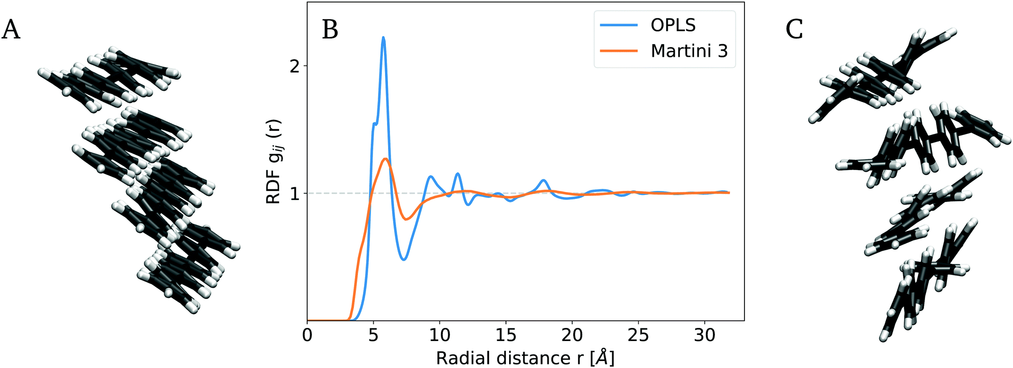
We next evaluated the properties of systems containing multiple PPE chains. To validate the Martini 3-based CG model presented here, we analyzed the local structural organization of PPE chains, and compared it to AA reference simulations and experimental measurements. To this end, we constructed and equilibrated a finite bundle of short PPE chains (10 chains, each 4 monomers in length), and monitored two major degrees of freedom, the radial arrangement of aligned polymers, and their axial displacement within the polymer bundle. These observables jointly tested the bonded and non-bonded interactions defined in the Martini 3 force field potential.

First, we characterized the radial displacement between PPE chains by computing the orthogonal distances between aligned polymer chains (eqn (4)). We determined the probability density for π stacking (Fig. 4A). The π stacking obtained from the AA and CG trajectories exhibits a similar behavior. In particular, we observed three distinct peaks of the distribution, at ∼ 0.5 nm, 0.8–0.9 nm and 1.2–1.3 nm. Both the AA and CG simulations show good agreement with the experimentally observed interchain distances.^82,83 Both models slightly overestimated the π stacking distances with reference to the experimental value (∼0.4 nm) by 15% for the first and 5% for the second and third peak. In contrast to the AA case, for Martini 3, the probability distribution did not drop to zero between the peaks, the second and third peaks were hardly separated, and finer structural features seen in the AA model were lost. This reflects an overall less ordered packing, which is expected, given the loss of resolution upon coarse-graining. To resolve the second and third peak in more detail, a finer resolution, i.e. mapping a ring of six heavy atoms to a rhombus of four beads, would be suitable at the expense of the performance. Still, the CG simulations capture the major features of radial packing of chains and, thus, yield the expected local structure of PPEs.

Fig. 4 Packing of aligned PPE molecules. (A) Radial orientation of aligned chains within the bundle estimated with the π stacking distance. Experimental measurements reported in the literature used for comparison.^82,83 (B) Axial displacement or side-by-side sliding of single chains within the polymer bundle. Both packing properties are validated with reference to OPLS atomistic data.²³

Second, we characterized the axial degree of freedom by computing the horizontal displacement of each chain relative to the centre of the polymer bundle. To this end, we projected the COM of each polymer onto the main COM axis of the bundle using eqn (5). We compared the probability densities from both AA and CG simulations as shown in Fig. 4B. Both the CG and AA models exhibit distributions around zero displacements with highly similar width. They both strongly disfavor chains from displacing relative to each other by more than 0.5 nm. Again, the CG model is unable to reproduce a finer Angstrom-scale structure of the PPEs, namely a bimodal distribution with peaks at ±0.13 nm. Aromatic rings slightly prefer an axial shift relative to one another by this length, a low-energy π stacking mode also known for benzene rings that the AA force field is able to capture.^34,84–86 In contrast, the probability density from Martini is unimodal and centered around mode zero. This deviation is due to the flattened free energy surface resulting from mapping the AA structure to the CG resolution, that is, a ring of six heavy atoms to a triangle of three beads. Yet, on the coarser scale beyond 1–2 Å, the CG data closely follows the AA data. Within the expected level of resolution of Martini, we conclude that our CG model accurately represents both the axial and radial degree of freedom within a bundle of aligned polymer chains.

3.6 Structural organization in PPE bulk systems

We next moved from finite PPE systems to a mid-size bulk PPE simulation system with full periodicity of the polymer material and absence of a solvent. The system size was chosen such that simulations at the atomistic scale are still feasible, and comprised 300 chains of 4 monomers each. To characterize the structural organization within a PPE bulk, we focused on properties at both the macroscopic and microscopic length scale, namely global packing by measuring the densities, and the local packing to short-range structural parameters. First, we evaluated the bulk densities from CG with AA simulations and obtained a bulk density of ρ_AA = 1092 kg m⁻³ and ρ_CG = 1098 kg m⁻³ for the AA and CG models, respectively (Fig. S4, ESI†). This agreement is satisfying, and suggests that the coarse-grained model largely reproduces the inter-PPE distances. Note that experimental densities for solid-state PPEs between 997 and 1118 kg m⁻³, obtained from X-Ray powder diffraction, depend strongly on the side-chain concentration, and are therefore not suited for validation purposes.^87,88

On the microscopic scale, we characterized the local organization within the bulk by computing the radial distribution function (RDF) for the assembly of 300 PPEs with a length of four monomers each. Fig. 5 shows a snapshot of the PPE bulk obtained from an AA system in A, from a backmapped CG system in C together with their respective RDF in B. For direct comparison, we mapped the AA and CG trajectory to a one-bead-per aromatic ring resolution and computed the RDF from the mapped trajectories to analyze the packing of 300 PPEs. Due to the symmetry along the backbone, the RDF between the triple bonds as well as the one between the aromatic and the ethynylene groups are very similar (Fig. S11, ESI†). For the mapped AA system, the RDF exhibits a first peak around 0.57 nm, a minimum at 0.73 nm, and a second and third peak at 0.92 and 1.13 nm, respectively. Hence, the PPE assembly, obtained from AA reference simulations, possesses a high degree of local order as shown in Fig. 5A. The RDF computed from the mapped Martini 3 trajectory exhibits a first peak at 0.58 nm, in close agreement with the AA force field. Its second maximum at 0.74 nm is broader and covers the second and third peaks of the RDF from the mapped AA trajectory. Thus, the Martini 3 model broadly shows a similar packing geometry also at such large distances. As expected and as also seen for finite bundles (Fig. 4), it is evident that the PPE assembly obtained on the CG scale is less locally ordered (Fig. 5C). As a consequence of this, the CG model for PPEs did not resolve features beyond the second peak. Still, overall, the packing of the first and second neighbors (i.e. first and second peaks in the RDF) is reproduced by the Martini 3 force field.

Fig. 5 Packing in mid-size bulk systems. (A) A snapshot of the AA trajectory indicates a high degree of local order. (B) Comparison of the RDF from mapped AA and CG simulations. The latter shows a less distinct pattern with lower order. (C) Backmapping from coarse- to fine grain resolution reveals a decrease in patterning. Local ordering of the nearest neighboring chains, given by the RDF's first two maxima, is reproduced by the CG force field.

3.7 Nematic alignment in large-scale bulk systems

The Martin 3 model now opens the route towards analyzing PPE assemblies at a larger length and time scale. We set out to construct simulation systems of 300 to 800 chains, with 20 to 60 monomers, resulting in box sizes of 10 nm³ to 20 nm³. In the largest system, around 200,000 CG beads represent approximately 600,000 atoms, and have been simulated for 5 microseconds (Fig. 6). Note that these spatial and temporal scales are already difficult to assess at the all-atom level of resolution.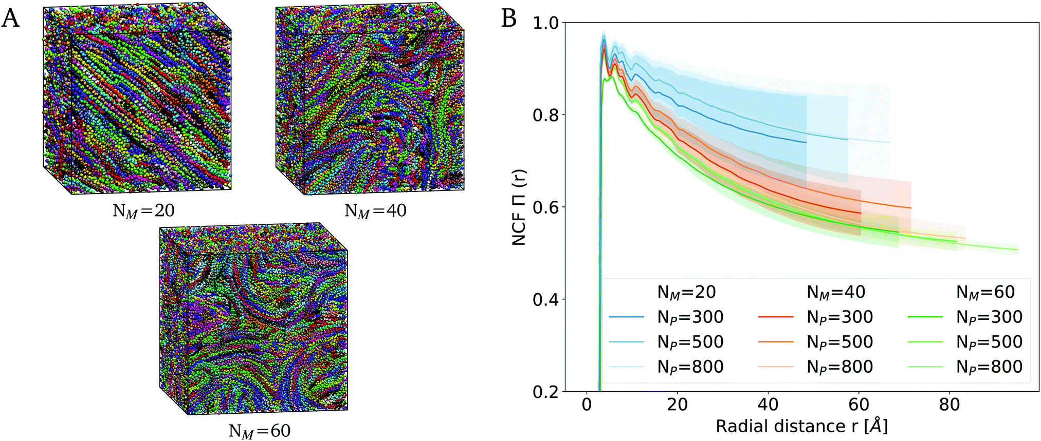

Fig. 6 Alignment in large-scale bulk systems. (A) Snapshots for bulk systems of 500 PPEs with a length of 20, 40 or 60 monomers. (B) Comparing the NCF for bulk systems of various numbers of monomers N_M and polymers N_P. Global ordering of PPEs decreases with increasing chain length.

Fig. 6A shows snapshots for a bulk system containing 500 PPEs consisting of 20, 40 and 60 monomers each. It is evident that short-chains mostly align in parallel, while this alignment is lost across larger distances when the chain length grows. To quantify this nanometer-scale alignment of polymers within the network, we calculated the nematic correlation function (NCF). The NCF describes the decay in structural order with increasing radial distance from a reference monomer, as defined in eqn (7). More precisely, the lower limit of the NCF (with 0.5) defines randomly oriented polymers and the upper one (with 1.0) parallelly oriented ones. Fig. 6B shows the results of the NCF analysis for different polymer chain lengths ranging from 20 to 60 monomers. We computed the average and standard deviation for the NCF from 8 replicas. The averaged NCF increases sharply at the beginning and decreases with increasing distance until the curve asymptotically approaches the lower limit of 0.5. As reflected by the standard deviations, the variations in nematic ordering reached after independent assembly simulations varied strongly for a given chain length and system size, as the ordering extends across length scales comparable to the system sizes.

Notwithstanding these fluctuations, the extensive sampling aided by the efficient Martini model allowed us to reveal significant differences when modifying the PPE chain length. Most importantly, we observe a steady decrease in ordering with increasing polymer chain length, across the whole range of radial distances. PPEs with a chain length in the range of their persistence length (20 monomers) show a higher degree of alignment in comparison to longer-chain PPEs (40 or 60 monomers). The latter are less parallel and rather assemble through entanglement as opposed to alignment. In this case, parallel alignment is maintained on a length scale of up to ∼5 nm, beyond which a nano-domain forms comprising PPE chains aligned along a different direction. The decrease in alignment with increase in polymer chain length can be attributed to the competition between entropic and enthalpic effects. The influence of the entropic effects on the polymer dynamics increases with the polymer length, thus long-chain PPEs exhibit a random coil-like behaviour with less ordering.

To exclude effects from the limited system size, we also examined the influence of the number of polymer chains on the NCF (Fig. 6B, lighter colors). We compared networks consisting of 300, 500 and 800 chains (e.g. system sizes of 12.1 nm³, 14.3 nm³ and 16.9 nm³ for a 40-monomer long chain), and found that the alignment of PPEs within a bulk system is constant with the increasing number of polymers, and hence independent of the box size. Starting from the equilibrated bulk structures, we confirmed our observation regarding the decrease in order with increasing chain length through annealing simulations of PPE networks (Fig. S12, ESI†).

Taken together, we observe a decay in nematic alignment of PPE chains on the nanometer length scale, resulting in the formation of nano-crystalline domains. The loss of interchain alignment is more pronounced for long-chain PPEs which form nano-domains on the ∼5 nm scale and are independent from the system size. Longer chains show more chain fluctuations and thus entanglement, which impedes the preferred interchain alignment observed for PPE chains with shorter chain lengths, i.e. lengths in the range of their persistence length.

4 Conclusions

In this paper, we have developed a Martini 3 model for the π conjugated backbone of PPEs which we validated against experimental properties for single chains and bulk mixtures, such as solvation and inter-chain packing. The CG model reproduced the stacking and axial displacement of polymers in a bundle as observed in AA reference simulations.^82,83 With the Martini 3 model at hand, we shed light on the structural properties of PPEs at larger length scales. As a proof of concept, we here found that the overall high nematic ordering is partly lost for longer chains (Fig. 6B). In addition, the assembly of polymers with chain lengths in the range of the persistence length exhibits parallel alignment across up to ∼6 nm.

We recommend the usage of the PPE Martini 3 model for understanding the bulk properties of PPEs, that is MD simulations compromising dozens of polymer chains, for which we observe a pronounced performance boost at the expense of structural detail. We compared the performance obtained with a single NVIDIA GeForce RTX 2080 Super GPU and a 20-core Intel Xeon Gold 6230 processor for the smallest bulk system, consisting of 300 polymers with 20 monomers each, for a total of 26,100 coarse-grained beads. Equilibration for this system, on a timescale of 5 microseconds, would take about 150 days at the AA level as opposed to 60 hours at the CG one. Obviously, the applicability of the AA or CG model depends on the dynamics the user wants to study. In general, the dynamics from Martini 3 simulations will allow the user to study larger polymer systems at longer timescales at the expense of loss on the atomistic accuracy.

The Martini 3 force field can be extended in a straightforward way to comprise side-chains of different chemistry (R in Fig. 1) to thereby analyze the packing of PPEs in detail. Future refinement of the already satisfying packing properties might involve a finer mapping scheme, a desolvation barrier potential, although no solvent molecule was found within the bundle of parallelly aligned polymer chains, or generic labels from Martini 3 to optimize self-interactions between phenyl rings.³⁴ Besides, backmapping the Martini 3 bulk systems to AA resolution allows an advanced analysis on different length scales depending on the required degree of detail. Therefore, our Martini 3 PPE model opens the pathway to elucidate the mechanical stress–strain response of PPE bulk systems under mechanical force as well as the microscopic interactions along the backbone. Finally, the CG model in combination with the backmapping routine and QM/MM methods could, e.g. help in understanding the electronic properties, conductance, or excited states in the environment found in bulk PPE networks.

Conflicts of interest

There are no conflicts to declare.

Acknowledgements

We are grateful for fruitful discussions with Peter Gumbsch and Florian Franz. We acknowledge funding through the Deutsche Forschungsgemeinschaft (DFG, German Research Foundation) under Germany's Excellence Strategy – 2082/1 – 390761711, the Klaus Tschira Foundation, the state of Baden-Württemberg through bwHPC and the DFG through grant INST 35/1134-1 FUGG.

References

1. U. H. F. Bunz, Acc. Chem. Res., 2001, 34, 998–1010.
2. H. Schnablegger, M. Antonietti, C. Göltner, J. Hartmann, H. Cölfen, P. Samori, J. P. Rabe, H. Häger and W. Heitz, J. Colloid Interface Sci., 1999, 212, 24–32.
3. T. M. Swager, C. J. Gil and M. S. Wrighton, J. Phys. Chem., 1995, 99, 4886–4893.
4. R. Deans, J. Kim, M. R. Machacek and T. M. Swager, J. Am. Chem. Soc., 2000, 122, 8565–8566.
5. Y. Jiang, D. Perahia, Y. Wang and U. H. F. Bunz, Macromolecules, 2006, 39, 4941–4944.
6. U. H. F. Bunz, K. Seehafer, M. Bender and M. Porz, Chem. Soc. Rev., 2015, 44, 4322–4336.
7. D. Perahia, R. Traiphol and U. H. F. Bunz, Macromolecules, 2001, 34, 151–155.
8. F. Markl, I. Braun, E. Smarsly, U. Lemmer, N. Mechau, G. Hernandez-Sosa and U. H. F. Bunz, ACS Macro Lett., 2014, 3, 788–790.
9. E. Smarsly, D. Daume, R. Tone, L. Veith, E. R. Curticean, I. Wacker, R. R. Schröder, H. M. Sauer, E. Dörsam and U. H. F. Bunz, ACS Appl. Mater. Interfaces, 2019, 11, 3317–3322.
10. J. H. Wosnick, C. M. Mello and T. M. Swager, J. Am. Chem. Soc., 2005, 127, 3400–3405.
11. J. H. Moon and T. M. Swager, Macromolecules, 2002, 35, 6086–6089.
12. B. Bagheri, M. Karttunen and B. Baumeier, Eur. Phys. J.: Spec. Top., 2016, 225, 1743–1756.
13. C. P. Broedersz and F. C. MacKintosh, Rev. Mod. Phys., 2014, 86, 995–1036.
14. P. M. Cotts, T. M. Swager and Q. Zhou, Macromolecules, 1996, 29, 7323–7328.
15. A. Godt, M. Schulte, H. Zimmermann and G. Jeschke, Angew. Chem., 2006, 118, 7722–7726.
16. F. Kienberger, V. P. Pastushenko, G. Kada, H. J. Gruber, C. Riener, H. Schindler and P. Hinterdorfer, Single Mol., 2000, 1, 123–128.
17. R. Ramachandran, G. Beaucage, A. S. Kulkarni, D. McFaddin, J. Merrick-Mack and V. Galiatsatos, Macromolecules, 2008, 41, 9802–9806.
18. C. Tweedie, G. Constantinides, K. Lehman, D. Brill, G. Blackman and K. Van Vliet, Adv. Mater., 2007, 19, 2540–2546.
19. D. Y. Yoon and P. J. Flory, J. Polym. Sci., Polym. Phys. Ed., 1976, 14, 1425–1431.
20. M. Das and F. C. MacKintosh, Phys. Rev. Lett., 2010, 105, 138102.
21. M. Das and F. C. MacKintosh, Phys. Rev. E: Stat., Nonlinear, Soft Matter Phys., 2011, 84, 061906.
22. C. J. Zeman and K. S. Schanze, J. Phys. Chem. A, 2019, 123, 3293–3299.
23. B. Bagheri, B. Baumeier and M. Karttunen, Phys. Chem. Chem. Phys., 2016, 18, 30297–30304.
24. M. Hodecker, A. M. Driscoll, U. H. F. Bunz and A. Dreuw, Phys. Chem. Chem. Phys., 2020, 22, 9974–9981.
25. S. Wijesinghe, S. Maskey, D. Perahia and G. S. Grest, J. Polym. Sci., Part B: Polym. Phys., 2016, 54, 582–588.
26. S. Maskey, J. M. D. Lane, D. Perahia and G. S. Grest, Langmuir, 2016, 32, 2102–2109.
27. S. J. Marrink, A. H. de Vries and A. E. Mark, J. Phys. Chem. B, 2004, 108, 750–760.
28. S. J. Marrink, H. J. Risselada, S. Yefimov, D. P. Tieleman and A. H. de Vries, J. Phys. Chem. B, 2007, 111, 7812–7824.
29. P. C. T. Souza, R. Alessandri, J. Barnoud, S. Thallmair, I. Faustino, F. Grünewald, I. Patmanidis, H. Abdizadeh, B. M. H. Bruininks, T. A. Wassenaar, P. C. Kroon, J. Melcr, V. Nieto, V. Corradi, H. M. Khan, J. Domański, M. Javanainen, H. Martinez-Seara, N. Reuter, R. B. Best, I. Vattulainen, L. Monticelli, X. Periole, D. P. Tieleman, A. H. de Vries and S. J. Marrink, Nat. Methods, 2021, 18, 382–388.
30. S. J. Marrink and D. P. Tieleman, Chem. Soc. Rev., 2013, 42, 6801.
31. R. Alessandri, F. Grünewald and S. J. Marrink, Cond. Mat. Mtrl. Sci., 2020, 33, 2008635.
32. N. Michelarakis, F. Franz, K. Gkagkas and F. Gräter, Phys. Chem. Chem. Phys., 2021, 23, 25901–25910.
33. F. Grünewald, R. Alessandri, P. C. Kroon, L. Monticelli, P. C. T. Souza and S. J. Marrink, Nat. Commun., 2022, 13, 68.
34. R. Alessandri, J. Barnoud, A. S. Gertsen, I. Patmanidis, A. H. de Vries, P. C. T. Souza and S. J. Marrink, Adv. Theory Simul., 2021, 2100391.
35. R. Alessandri, P. C. T. Souza, S. Thallmair, M. N. Melo, A. H. de Vries and S. J. Marrink, J. Chem. Theory Comput., 2019, 15, 5448–5460.
36. F. Grunewald, G. Rossi, A. H. de Vries, S. J. Marrink and L. Monticelli, J. Phys. Chem. B, 2018, 122, 7436–7449.
37. H. J. Risselada, Nat. Methods, 2021, 18, 342–343.
38. J. J. Uusitalo, H. I. Ingólfsson, P. Akhshi, D. P. Tieleman and S. J. Marrink, J. Chem. Theory Comput., 2015, 11, 3932–3945.
39. J. Sangster, J. Phys. Chem. Ref. Data, 1989, 18, 1111–1229.
40. C. Hansch, A. Leo and D. Hoekman, Exploring QSAR Vol. 2: Hydrophobic, electronic, and steric constants, American Chemical Society, Washington, DC, 1995.
41. E. Lindahl, M. J. Abraham, B. Hess and D. van der Spoel, GROMACS 2020 Source code (2020), Zenodo, 2020 DOI:10.5281/zenodo.3923645.
42. K. Okuyama, T. Hasegawa, M. Ito and N. Mikami, J. Phys. Chem., 1984, 88, 1711–1716.
43. C. E. Halkyard, M. E. Rampey, L. Kloppenburg, S. L. Studer-Martinez and U. H. F. Bunz, Macromolecules, 1998, 31, 8655–8659.
44. S. Toyota, Chem. Rev., 2010, 110, 5398–5424.
45. E. Lindahl, M. J. Abraham, B. Hess and D. van der Spoel, GROMACS 2020 Manual (2020), Zenodo, 2020 DOI:10.5281/zenodo.3562512.
46. G. Bussi, D. Donadio and M. Parrinello, J. Chem. Phys., 2007, 126, 014101.
47. M. Parrinello and A. Rahman, J. Appl. Phys., 1981, 52, 7182–7190.
48. S. Pall and H. Berk, Phys. Comp., 2013, 1–17.
49. T. Darden, D. York and L. Pedersen, J. Chem. Phys., 1993, 98, 10089–10092.
50. U. Essmann, L. Perera, M. L. Berkowitz, T. Darden, H. Lee and L. G. Pedersen, J. Chem. Phys., 1995, 103, 8577–8593.
51. N. Goga, A. J. Rzepiela, A. H. de Vries, S. J. Marrink and H. J. C. Berendsen, J. Chem. Theory Comput., 2012, 8, 3637–3649.
52. G. J. Martyna, D. J. Tobias and M. L. Klein, J. Chem. Phys., 1994, 101, 4177–4189.
53. D. H. de Jong, S. Baoukina, H. I. Ingólfsson and S. J. Marrink, Comput. Phys. Commun., 2016, 199, 1–7.
54. Martini, General Purpose Coarse-Grained Force Field, 2021, http://www.cgmartini.nl/.
55. P. C. T. Souza, S. Thallmair, P. Conflitti, C. Ramírez-Palacios, R. Alessandri, S. Raniolo, V. Limongelli and S. J. Marrink, Nat. Commun., 2020, 11, 3714.
56. F. Grünewald, P. C. Kroon, P. C. T. Souza and S. J. Marrink, Structural Genomics, Springer US, New York, NY, 2021, vol. 2199, pp. 315–335.
57. S. Kirkpatrick, C. Gelatt and M. Vecchi, Science, 1983, 220, 671–680.
58. R. Alessandri, J. J. Uusitalo, A. H. de Vries, R. W. A. Havenith and S. J. Marrink, J. Am. Chem. Soc., 2017, 139, 3697–3705.
59. R. Alessandri, S. Sami, J. Barnoud, A. H. Vries, S. J. Marrink and R. W. A. Havenith, Adv. Funct. Mater., 2020, 30, 1–11.
60. C.-H. Shu, M.-X. Liu, Z.-Q. Zha, J.-L. Pan, S.-Z. Zhang, Y.-L. Xie, J.-L. Chen, D.-W. Yuan, X.-H. Qiu and P.-N. Liu, Nat. Commun., 2018, 9, 2322.
61. C. C. Bannan, G. Calabró, D. Y. Kyu and D. L. Mobley, J. Chem. Theory Comput., 2016, 12, 4015–4024.
62. S. Kumar, J. M. Rosenberg, D. Bouzida, R. H. Swendsen and P. A. Kollman, J. Comput. Chem., 1992, 13, 1011–1021.
63. J. S. Hub, B. L. de Groot and D. van der Spoel, J. Chem. Theory Comput., 2010, 6, 3713–3720.
64. N. Nitschke, K. Atkovska and J. S. Hub, J. Chem. Phys., 2016, 145, 125101.
65. R. Gowers, M. Linke, J. Barnoud, T. Reddy, M. Melo, S. Seyler, J. Domański, D. Dotson, S. Buchoux, I. Kenney and O. Beckstein, MDAnalysis: A Python Package for the Rapid Analysis of Molecular Dynamics Simulations, Austin, Texas, 2016, pp. 98–105.
66. N. Michaud-Agrawal, E. J. Denning, T. B. Woolf and O. Beckstein, J. Comput. Chem., 2011, 32, 2319–2327.
67. C. R. Harris, K. J. Millman, S. J. van der Walt, R. Gommers, P. Virtanen, D. Cournapeau, E. Wieser, J. Taylor, S. Berg, N. J. Smith, R. Kern, M. Picus, S. Hoyer, M. H. van Kerkwijk, M. Brett, A. Haldane, J. F. del Río, M. Wiebe, P. Peterson, P. Gérard-Marchant, K. Sheppard, T. Reddy, W. Weckesser, H. Abbasi, C. Gohlke and T. E. Oliphant, Nature, 2020, 585, 357–362.
68. H.-P. Hsu, W. Paul and K. Binder, Macromolecules, 2010, 43, 3094–3102.
69. P. Gutjahr, R. Lipowsky and J. Kierfeld, Europhys. Lett., 2006, 76, 994–1000.
70. H.-P. Hsu, W. Paul and K. Binder, Polym. Sci., Ser. C, 2013, 55, 39–59.
71. H. Benoit and P. Doty, J. Phys. Chem., 1953, 57, 958–963.
72. M. Doi, S. F. Edwards and S. F. Edwards, The Theory of Polymer Dynamics, Clarendon Press, 1988.
73. P. Virtanen, R. Gommers, T. E. Oliphant, M. Haberland, T. Reddy, D. Cournapeau, E. Burovski, P. Peterson, W. Weckesser, J. Bright, S. J. van der Walt, M. Brett, J. Wilson, K. Millman, N. Mayorov, A. R. Nelson, E. Jones, R. Kern, E. Larson, C. Carey, I. Polat, Y. Feng, E. Moore, J. VanderPlas, D. Laxalde, J. Perktold, R. Cimrman, I. Henriksen, E. Quintero, C. R. Harris, A. M. Archibald, A. H. Ribeiro, F. Pedregosa and P. van Mulbregt, Nat Methods, 2020, 17(3), 261–272.
74. J. B. Carrell, Groups, Matrices, and Vector Spaces: A Group Theoretic Approach to Linear Algebra, Springer New York, New York, NY, 2017.
75. M. L. Waskom, Journal of Open Source Software, 2021, 6(60), 3021.
76. M. Tuckerman, Statistical Mechanics: Theory And Molecular Simulation, Oxford University Press, Oxford, 2010.
77. R. Fitzpatrick, D. Michieletto, K. R. Peddireddy, C. Hauer, C. Kyrillos, B. J. Gurmessa and R. M. Robertson-Anderson, Condens. Matter, 2018, 257801-1-7.
78. T. Bereau and K. Kremer, J. Chem. Theory Comput., 2015, 11, 2783–2791.
79. J. A. Graham, J. W. Essex and S. Khalid, J. Chem. Inf. Model., 2017, 57, 650–656.
80. C. Empereur-Mot, L. Pesce, G. Doni, D. Bochicchio, R. Capelli, C. Perego and G. M. Pavan, ACS Omega, 2020, 5, 32823–32843.
81. F. Eisenhaber, P. Lijnzaad, P. Argos, C. Sander and M. Scharf, J. Comput. Chem., 1995, 16, 273–284.
82. L. Kloppenburg, D. Jones, J. B. Claridge, H.-C. zur Loye and U. H. F. Bunz, Macromolecules, 1999, 32, 4460–4463.
83. D. Ofer, T. M. Swager and M. S. Wrighton, Chem. Mater., 1995, 7, 418–425.
84. M. O. Sinnokrot and C. D. Sherrill, J. Phys. Chem. A, 2004, 108, 10200–10207.
85. T. M. Cardozo, A. P. Galliez, I. Borges, F. Plasser, A. J. A. Aquino, M. Barbatti and H. Lischka, Phys. Chem. Chem. Phys., 2019, 21, 13916–13924.
86. J. Hermann, D. Alfè and A. Tkatchenko, Nat. Commun., 2017, 8, 14052.
87. U. H. F. Bunz, V. Enkelmann, L. Kloppenburg, D. Jones, K. D. Shimizu, J. B. Claridge, H.-C. zur Loye and G. Lieser, Chem. Mater., 1999, 11, 1416–1424.
88. H. Li, D. R. Powell, R. K. Hayashi and R. West, Macromolecules, 1998, 31, 52–58.

---

Footnote

† Electronic supplementary information (ESI) available: Coarse-grained distributions and bulk densities for center-of-geometry or geometrical mapping, potential of mean forces, and persistence length estimation. See DOI: 10.1039/d1cp04237h

---