On standardised moments of force distribution in simple liquids†
Received
3rd September 2021
, Accepted 26th January 2022
First published on 27th January 2022
Abstract
The force distribution of a tagged atom in a Lennard-Jones fluid in the canonical ensemble is studied with a focus on its dependence on inherent physical parameters: number density (n) and temperature (T). Utilising structural information from molecular dynamics simulations of the Lennard-Jones fluid, explicit analytical expressions for the dependence of standardised force moments on n and T are derived. Leading order behaviour of standardised moments of the force distribution are obtained in the limiting cases of small density (n → 0) and low temperature (T → 0), while the variations in the standardised moments are probed for general n and T using molecular dynamics simulations. Clustering effects are seen in molecular dynamics simulations and their effect on these standardised moments is discussed.
I. Introduction
Understanding the moments and measures of a distribution for a fully atomistic molecular dynamics (MD) simulation allow us to better fit coarser models that reproduce these.1–3 It is often the case in model coarse-graining that we wish to directly reconcile the energy landscape of the fully atomistic system to a more basic representation that allows us to maintain as many physical properties of the system of interest, with as little computational cost as possible.4 Though, it is also natural to match forces between the high and low resolution systems in an effort to reproduce the force distribution which will inherently give rise to the energy landscape.5–10
Let F = [F1, F2, F3] denote a force on a tagged atom in a liquid. Depending on the relative positions of other atoms, force F can vary over a range of values and a detailed information on F can be obtained by calculating properties of its equilibrium distribution, which we will call force distribution in this manuscript. Considering an isotropic system, the equilibrium distribution of each force coordinate is the same. We define the standardised moment of the force distribution by averaging over the k-th power of its first coordinate as
| |  | (1) |
where 〈
Fk1〉 is the
k-th moment of the force distribution and
αk standardises the
k-th moment by scaling it with the
k-th power of the standard deviation of the force distribution. In a simple homogeneous fluid with radially symmetric interactions between particles, the force distribution will exhibit symmetry around the origin and thus all odd standardised moments vanish,
i.e. 0 =
α1 =
α3 =
α5 = ⋯. As
α2 ≡ 1 by definition
(1), the first non-trivial standardised moment is kurtosis, denoted
α4, which provides a measure of spread that details how tailed the force distribution is relative to a normal distribution.
11 In this paper, we study how the force distribution depends on the number density of a homogeneous many-body system, and the temperature of the same system in a canonical ensemble. We will do this by studying the behaviour of the second moment of the force distribution 〈
F12〉 and standardised even moments
α4,
α6,
α8,…. If the force distribution was Gaussian, then the even standardised moments would be
| |  | (2) |
and the second moment 〈
F12〉 would be sufficient to parametrize the force distribution. However, the force distributions in simple liquids have been reported to deviate from Gaussian distribution.
12–14 In particular, by comparing the results of our analysis with Gaussian moments in
eqn (2), we can also quantify how non-Gaussian the real force distribution is.
Much work has been done in the area of force distributions of many-body systems: with seminal work from Chandrasekhar15 that employed Markov's theory of random flights to give an expression for the force distribution of a many-body system interacting through a 1/r gravitational potential. More recent work has been done with the help of MD by Gabrielli et al.,16 who derived an expression for the kurtosis of the force distribution for a lattice system of atoms interacting through the gravitational potential. Further, using the classical density functional theory, an expression for the probability distribution of force for a system interacting through an arbitrary weakly repulsive potential was derived by Rickayzen et al.17,18
In this paper, we study the number density and temperature dependence of the force distribution for a many-body system interacting through a Lennard-Jones 12-6 potential,19,20 which is ubiquitously used and has been shown to model homogeneous systems of interacting (Argon) atoms well.21–23
In Section III, an in depth investigation is given to the simple two-body system in one spatial dimension, which provides the ideal platform to illustrate the underlying methods while retaining interesting dynamical behaviour. From first principles we derive first-order partial differential equations (PDEs) describing the parameter dependence of the standardised moments of the force distribution. In doing so we further derive an analytic expression for the partition function of a two-body system that depends solely on the standardised moments of the force distribution whereupon the expression is exact in an asymptotic limit of the density going to zero (n → 0). Similarly, an expression is derived relating the average energy of the system to standardised moments of force from the temperature dependent PDE. In parameter regimes where long-range forces between atoms dominate, we use a truncated Taylor series expansion to derive the leading order behaviour of the kurtosis of the force distribution in the limit n → 0. Finally, we utilise a Laplace integral approximation to ascertain the leading order behaviour of the standardised moments of force at low temperatures (T → 0). Results from simple MD simulations are presented to provide evidence for the efficacy of these methods and underlying assumptions.
This is followed by Section IV, where the natural idea that long range force calculations dictate asymptotic behaviour is extended from the 1D model to many-body systems of arbitrary size in three spatial dimensions. These systems exhibit the physical properties of standard MD simulations: i.e. cubic geometry with periodic boundary conditions that employ the minimum image convention. In particular, we can analyze the system by performing calculations on a central cubic cell. In Section IV.B, MD results are displayed for many-body systems. We present the dependence of the standardised force moments on density, n, and temperature, T, and discuss the parameters and integrator schemes utilised in producing the results of MD simulations.
II. Notation
We consider a system of N identical atoms interacting via the Lennard-Jones 12-6 potential.19 This is a ubiquitous inter-atomic pairwise potential; here the potential between atoms labelled i, j = 1, 2,…, N positioned at qi, qj ∈ ![[Doublestruck R]](https://www.rsc.org/images/entities/char_e175.gif) 3 is given (in reduced units24) by the expression
3 is given (in reduced units24) by the expression| |  | (3) |
where rij = |qi − qj| is the distance between atoms. The Lennard-Jones potential (3) between two atoms has a unique minima obtained at rij = r* = 21/6.
We employ the framework of statistical mechanics for this closed many-body system and describe atom i = 1, 2,…, N by phase space coordinates {qi, pi} ∈ ![[Doublestruck R]](https://www.rsc.org/images/entities/char_e175.gif) 6, were pi denotes the momentum of the i-th atom. We work in the canonical ensemble with temperature T; the partition function therefore becomes
6, were pi denotes the momentum of the i-th atom. We work in the canonical ensemble with temperature T; the partition function therefore becomes
| |  | (4) |
where
V is the volume of our closed system, and
q = (
q1,
q2,…,
qN)
T and
p = (
p1,
p2,…,
pN)
T are vectors containing the positions and momenta of all atoms in the system. Our integration domain is given by
Ωq ×
Ωp ⊂
![[Doublestruck R]](https://www.rsc.org/images/entities/char_e175.gif) 3N
3N ×
![[Doublestruck R]](https://www.rsc.org/images/entities/char_e175.gif) 3N
3N. This denotes the phase space of our system. For systems of interest
Ωp ≡
![[Doublestruck R]](https://www.rsc.org/images/entities/char_e175.gif) 3N
3N. The underlying geometry of the system (and principle simulation cell) is a cubic box of size
L > 0, therefore
Ωq ≡ (−
L/2,
L/2] × … × (−
L/2,
L/2]. The phase space volume elements in
eqn (4) are denoted by
| |  | (5) |
Throughout this work we make use of reduced units,
24 utilising Argon parameters.
25 In particular, all instances of
T in this work can be translated back to SI units with the transformation
T →
kBT where
kB is the Boltzmann factor. Therefore, in the partition function
(4), we have
β = 1/
T and
h is the Planck constant (≈0.186 in reduced units). Finally,
H(
q,
p) is the classical Hamiltonian
H(
q,
p) =
K(
p) +
U(
q) with kinetic energy
K(
p) = |
p|
2/2 (where the usual factor of mass is unity under reduced units) and a general potential
U(
q). The statistical average of a quantity
X for this
N-body system is given by
| |  | (6) |
where the Boltzmann factor acts as a statistical weighting for a configuration {
q,
p} ∈
![[Doublestruck R]](https://www.rsc.org/images/entities/char_e175.gif) 6N
6N, normalised such that 〈1〉 = 1.
We label atoms so that the first one is the tagged atom. Denoting the force on the tagged atom produced from the j-th atom by Fj = [Fj,1, Fj,2, Fj,3] ∈ ![[Doublestruck R]](https://www.rsc.org/images/entities/char_e175.gif) 3, for j = 2, 3,…, N, the total force F = [F1, F2, F3] on the tagged atom is
3, for j = 2, 3,…, N, the total force F = [F1, F2, F3] on the tagged atom is
We define
| |  | (7) |
for
k = 0, 1, 2,… Then we have
Then the
k-th standardised moment
(1) is given by
| |  | (8) |
where we are interested in cases
k = 4, 6, 8,….
In order to study how the force distribution depends on the physical parameters of interest it is useful to identify how changes in these parameters will manifest themselves in the system. Indeed, we choose to work in the canonical ensemble with a target temperature of T: this is accomplished with the use of a thermostat which is discussed further in Section IV.B and Appendix B. It is more illuminating to see that if we have a system with a fixed number of free interacting atoms N in a cubic box of side L; the (reduced) number density is given by n = N/L3. Therefore the approach we employ in this paper to ascertain how values of standardised moments depend on number density, will be to keep the number of atoms fixed but vary the box width L – this will manifest as a change in density n. Similarly one could keep the volume of the cubic box the same and vary the number of atoms though this is a point of discussion in Section IV.B.
For the remainder of the paper we will study systems with different spatial dimensions. The size of the system varies by changing the number of particles N; we will use eqn (8) as a crucial initial point in each calculation. We will naturally proceed by investigating systems of increasing complexity; starting from a cartoon one-dimensional model and culminating to a general many-body system of arbitrary size in three spatial dimensions.
III. One atom in a potential well
We now go on to illustrate three approaches to obtain the dependence of the force distribution on parameters n and T. It is useful to note that, as we are now working in one spatial dimension, density n is proportional to 1/L, i.e. we have n ∝ 1/L. We will consider a simple system in one spatial dimension consisting of two atoms interacting through the Lennard-Jones potential (3) in interval [0, L] with periodic boundary conditions. One of the atoms is considered to be fixed at position q0 = L/2 ∈ [0, L] and the other atom is free to move, therefore, we have N = 1 free atom. Its position is denoted x ∈ [0, L]. Therefore, the inter-atomic distance is r = |x − q0|. Using our simplified one-dimensional set up, F1 = F and Ωq = (0, L), eqn (7) reduces to| |  | (9) |
which is the marginalised expected value of the k-th moment of force F(x) = −dU/dx, where we have dropped subscripts in the Lennard-Jones potential (3) and we write it as U(z) = 4(z−12 − z−6). Utilising the symmetry of the potential (and therefore the force) we are left with| |  | (10) |
In what follows, we will assume that we are in a regime where the box width L satisfies L ≫ r*, where r* = 21/6 minimizes the Lennard-Jones potential U.
A. Differential equation for standardised moments
We consider a perturbation of the form L → L + δL. Using eqn (10) and considering terms to the order O(δL), we obtain
Using eqn (8), we approximate αk(L + δL) by
αk(L) + αk(L) νk(L)![[thin space (1/6-em)]](https://www.rsc.org/images/entities/char_2009.gif) exp[−βU(L/2)] δL + O(δL2), exp[−βU(L/2)] δL + O(δL2), |
where our notation αk(L) highlights the dependence of the standardised moments of force, αk, on L, and function νk(L) is given by| |  | (11) |
Taking the limit δL → 0, we obtain the derivative of the k-th standardised moment of force, with respect to L, as| |  | (12) |
where νk(L) are expressed in terms of integrals (10) as given by eqn (11).
B. Far-field integral approximation
To further analyze integrals (10), we introduce a cutoff c, which satisfies that r* < c < L/2, where r* = 21/6 is a unique maximum of exp[−βU(z)], which can be Taylor expanded as β(1 + 4z−6 + 4z−12 − 16/3z−18 + 8z−24…). Considering sufficiently large L, we can choose the cutoff c, so that| |  | (13) |
where tolerance ε is chosen to be 10−4 in our illustrative computations. This splitting allows us to numerically calculate the bulk of the integral (10) as a constant independent of L and then use the second term to give an analytic expression for αk with dependence on L, and ultimately on n.
The range of values of T that are of typical use are chosen in order to maintain the liquid state of Argon during simulation. These are approximately temperatures in the interval 0.70 < T < 0.73 under ambient conditions.26 Therefore, as volume is varied we are in a regime where β = O(1), for convenience we set β = 1. Though given that the density of our system changes between each simulation some systems will be in a liquid phase and others in a gaseous phase, this is a point of discussion in Section IV.B.
Splitting the integration domain [0, L/2] of integral (10) into [0, c] and [c, L/2], we use the exact form of the integrand in [0, c] to obtain a ‘near-field’ contribution. Utilising an approximate form for the integrand given by the truncated Taylor expansion f(z) in the domain [c, L/2] gives rise to a density dependent ‘far-field’ contribution. Combining these we arrive at the approximate form for f0(L). Using cutoff c = 2, eqn (13) is satisfied with ε = 10−4. Therefore, upon numerically calculating the bulk contribution for the integral with domain [0, 2], we get
| |  | (14) |
with
b0 = −0.71832, which depends on our choice of cutoff
c = 2. Similarly, we can calculate far-field integral approximations of integrals
(10) for general values of
k = 2, 4, 6, 8, 10, 12. The integrand
Fk(
r)
![[thin space (1/6-em)]](https://www.rsc.org/images/entities/char_2009.gif)
exp[−
βU(
r)] has maxima when
r =
r* = 2
1/6 or when
kU′′(
r) =
β(
U′(
r))
2. This forms a cubic in
r6 that can be solved. For the values of
k used in this work, this sometimes results in a global maximum, that always lies at a distance less than
r <
r* from the origin. Therefore
r* = 2
1/6 is the furthest maximum of the integrand from the origin.
Splitting integral (10) into a near-field and far-field contribution, using the general cutoff c = 2, we find
The near-field contributions,
bk, generally increase vastly if we increase the value of
k, for example
| | | b0 = −0.71832, b2 = 130.64 and b4 = 2.5727 × 10⁵, | (16) |
while the dependence on
L decreases more rapidly for larger values of
k. Therefore, the non-negligible density contributions to
αk(
L) in the low density limit come exclusively from the normalisation
f0(
L) given by
(14).
Substituting eqn (14) and (15) in eqn (8), we obtain an expression for the general k-th standardised moment of force
| |  | (17) |
Using the values of
b0,
b2 and
b4 given by
(16), we obtain the dependence of the kurtosis of the force distribution on the reduced number density
n = 1/
L in the dilute limit
n → 0 as
α4 = −10.828 + 15.074
n−1 +
O(
n6).
Fig. 1 compares this result with the results obtained by MD simulation of the one atom system. We observe that MD is in good agreement with the results obtained by formula
(17).
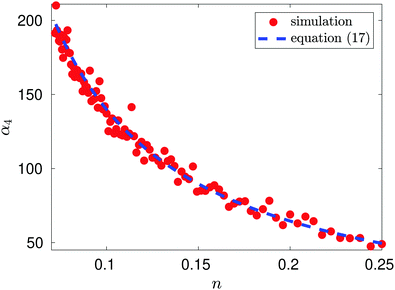 |
| | Fig. 1 Plot of α4 as a function of n = 1/L for the illustrative one-atom system. Results of MD simulations are compared with α4 = −10.828 + 15.074n−1 obtained by using eqn (17) with b0, b2 and b4 given by (16) (blue dashed line). MD simulation results for temperature T = 1 utilising Langevin dynamics27 described in eqn (B1), with friction parameter γ = 0.1, are represented by red dots. The MD simulation length was a total of 1.1 × 10⁸ time steps with the first 107 time steps used for initialisation. | |
C. Leading order behaviour for differential eqn (12)
Since L/2 > r*, the force F (L/2) monotonically decreases as a function of L. When looking at leading order approximations in the low density limit n → 0 (equivalent to limit L → ∞) to eqn (12), we need to analyse νk(L). The second and third term in eqn (11) converge to zero more rapidly than the first term as L → ∞, therefore the leading order behaviour is given by the first term| |  | (18) |
By utilising the far field integral approximation (14), we arrive at f0(L) ∼ (b0 + L), where b0 = b0(c) is a constant term that depends on cutoff parameter c. With this, our leading order approximation of the k-th standardised moment, α0k, obeys
Finally this gives us that| | | α0k(L) = Ck (b0 + L)k/2−1 = Ck (b0 + n−1)k/2−1, | (19) |
where n = 1/L is the reduced number density and Ck is a constant. Eqn (19) gives the same leading order behaviour n1−k/2 in the limit n → 0 as eqn (17): the same behaviour is also seen for the Lennard-Jones fluid in Section IV. Though the method above is more generally applicable to include potentials that monotonically decay as r−a as r → ∞ for a > 0. We next make the observation that eqn (4) in 1D can be written as:| |  | (20) |
where the Planck factor of 1/h arises instead of 1/h3 due to the fact that we are in one-dimensional physical space. Using (10), we obtain| |  | (21) |
Considering the low density limit n → 0 (i.e. L → ∞) in eqn (12) and using (18) and (21), we obtain| |  | (22) |
as L → ∞. In particular, we can obtain the partition function (20) in the dilute (low density) limit by using information about the moments of the force distribution. The accuracy of eqn (22) is illustrated in Fig. 2, where we use k = 4. We use MD simulations of a single atom, using a range of simulation box widths L. We estimate the values of kurtosis of the force distribution, its derivative with respect of L and use the right hand side of eqn (22) to estimate the ![[scr Z, script letter Z]](https://www.rsc.org/images/entities/char_e14b.gif) 1(T, V). Considering L ≥ 10, the result is within 5% error when compared with the exact result (20), while for larger values of box width L the error decreases to around 1%, confirming that the formula (22) is valid in the asymptotic limit L → ∞.
1(T, V). Considering L ≥ 10, the result is within 5% error when compared with the exact result (20), while for larger values of box width L the error decreases to around 1%, confirming that the formula (22) is valid in the asymptotic limit L → ∞.
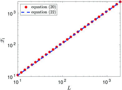 |
| | Fig. 2 Approximation of the partition function ![[scr Z, script letter Z]](https://www.rsc.org/images/entities/char_e14b.gif) 1(T, V) obtained using the right hand side of eqn (22) with k = 4 and values of kurtosis (α4) estimated from MD simulation (blue dashed line). The exact values obtained by eqn (20) are plotted as the red dots. 1(T, V) obtained using the right hand side of eqn (22) with k = 4 and values of kurtosis (α4) estimated from MD simulation (blue dashed line). The exact values obtained by eqn (20) are plotted as the red dots. | |
D. Temperature dependence of standardised moments
One can perform a similar analysis as in Section III.A, viewing the moments αk = αk(T) as a function of temperature T = 1/β. To do that, we consider the moment definition (10) as a function of temperature T, namely, we define| |  | (23) |
Considering small perturbations of these functions with respect to T → T + δT, while fixing the domain length L, and collecting terms up to first order in δT, we obtain| |  | (24) |
where| |  | (25) |
Combining eqn (24) and (25) with eqn (21) where β = 1/T, we obtain
Since −∂/∂β(ln![[thin space (1/6-em)]](https://www.rsc.org/images/entities/char_2009.gif)
![[scr Z, script letter Z]](https://www.rsc.org/images/entities/char_e14b.gif) 1) is equal to the average energy of the system, 〈E〉, we have
1) is equal to the average energy of the system, 〈E〉, we have| |  | (26) |
where the first term on the right hand side of eqn (26) is the average kinetic energy of our one-atom system. Substituting eqn (8) into the second term on the right hand side, it can be rewritten as T2 ∂(ln![[thin space (1/6-em)]](https://www.rsc.org/images/entities/char_2009.gif) f0)/∂T. Thus, using eqn (6), we confirm that the second term on the right hand side of eqn (26) is the average potential energy.
f0)/∂T. Thus, using eqn (6), we confirm that the second term on the right hand side of eqn (26) is the average potential energy.
E. Low temperature limit
Next, we consider the behaviour of the k-th standardised moment of force, αk(T), given by eqn (8), in the low temperature limit, T → 0, which is equivalent to the limit β → ∞. Since the inter-atomic potential U(r) has a global minimum at r = r* in interval [0, L/2], integrals of the form (10) and (23) can be approximated by Laplace's method in the limit β → ∞ and T → 0, respectively. A general discussion of Laplace's method is given in Chapter 6 of the book by Bender and Orszag.28 We calculate the asymptotic expansion of f0(T) by applying Laplace's method to integral (23) for k = 0. We approximate the integration limits of integral (23) to lie within the domain r ∈ (r* − ε, r* + ε), where ε ≪ 1, and we Taylor expand U(r) at r = r*. Using U′(r*) = 0, we have
where we denote the m-th derivative of U as U(m) for m ≥ 3. Substituting into integral (23), we arrive at the asymptotic expansion| |  | (27) |
as T → 0, where constant B0 is given by28| |  | (28) |
To apply Laplace's method to integral (23) for k = 2, 4, 6,…, we note that Fk(r) = (U′(r))k for even values of k. Using the truncated Taylor expansion around r = r* and noting that U′(r*) = 0, we have| | | Fk(r) ≈ (r − r*)k ((U′′(r*))k + (r − r*) Ck,1 + (r − r*)2Ck,2), | (29) |
where Ck,1 and Ck,2 are constants, which can be expressed in terms of the derivatives of potential U(r) at r = r* (see eqn (A1) and (A2) in Appendix A). This gives the asymptotic expansion| |  | (30) |
as T → 0, where constants Ak and Bk are given by
| Ak = (U′′(r*))k/2(k − 1)!! |
and
where the last formula reduces to eqn (28) for k = 0. Substituting (27) and (30) into (8) gives the following expression in the limit T → 0:
In particular, we have α2 ∼ 1 + O(T2) and| |  | (31) |
Therefore, Laplace's method predicts that the standardised moments of the force distribution, αk(T), tend to the values given in eqn (2) for Gaussian moments in the low temperature limit. This limiting behaviour is to be expected as during the Laplace approximation we use a Gaussian distribution to approximate the Boltzmann factor. We can interpret this approach as approximating the force distribution as Gaussian and perturbations of the system around small temperatures give rise to non-Gaussian contributions to the standardised moments.
Results from MD simulation are illustrated in Fig. 3 over the range of values of temperature T. We see that the behaviour of kurtosis, α4, is well approximated by the linear approximation 3 + 203 T/6 given in eqn (31) for the temperature values satisfying T ≤ 0.1, though this agreement diverges as temperature T increases and higher order terms, O(T2) in eqn (31), become significant. In Fig. 3, we fix the box width as L = 10. Increasing the box width much further would take us to a regime where the particle is essentially free and the approximation calculated by the Laplace method around the potential minimum would lose validity.
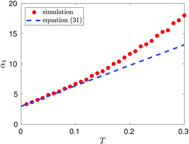 |
| | Fig. 3 Kurtosis, α4, as a function of temperature, T, for T ≤ 0.3. The linear behaviour is estimated as α4(T) ∼ 2.9388 + 37.002T for T ∈ (0.01, 0.10) (using the MD computed data, with density n = 0.1, visualized as red dots). We compare this to the theoretical linear result 3 + 203 T/6 predicted by eqn (31) (illustrated by the blue dashed line). | |
IV. Many-body systems
In this section we employ the far field approximation approach introduced in Section III.B and we will vary the number density of the system by changing the size L of the integration domain, which will be given as the three-dimensional cube [0, L]3. Using notation introduced in Section II, the distance between atoms labelled i, j = 1, 2,…, N positioned at qi, qj ∈ ![[Doublestruck R]](https://www.rsc.org/images/entities/char_e175.gif) 3 is denoted by rij = |qi − qj|. Taking into account the periodic boundary conditions, the distance |qi − qj| is the minimum image inter-atomic distance given by
3 is denoted by rij = |qi − qj|. Taking into account the periodic boundary conditions, the distance |qi − qj| is the minimum image inter-atomic distance given by| |  | (32) |
where the overline denotes ![[small xi, Greek, macron]](https://www.rsc.org/images/entities/char_e0cf.gif) = ζ−L [ζ/L] for ζ ∈
= ζ−L [ζ/L] for ζ ∈ ![[Doublestruck R]](https://www.rsc.org/images/entities/char_e175.gif) and [·] rounds a real number to the nearest integer. For an interacting N-body system the dimensionality of the integral given by eqn (7) is 3N. We first present an illustrative calculation with N = 2 interacting atoms in Section IV.A and then we study systems with larger values of N in Section IV.B.
and [·] rounds a real number to the nearest integer. For an interacting N-body system the dimensionality of the integral given by eqn (7) is 3N. We first present an illustrative calculation with N = 2 interacting atoms in Section IV.A and then we study systems with larger values of N in Section IV.B.
A. Dependence of αk on density for N = 2 interacting atoms
In Section III, we have considered two atoms in the one-dimensional spatial domain, where one atom was fixed at position q0, i.e. we have effectively studied a single atom in a one-dimensional potential well. Here, we will consider N = 2 interacting atoms in the three-dimensional cubic domain [0, L]3 with periodic boundary conditions. We calculate the k-th standardised moment of force according to eqn (8). To do so, we consider eqn (7), where we have d3q = d3q1 d3q2, U(q) = U(r12), F1(q) = F1(r12) and we integrate over the domain Ω = [0, L]3 × [0, L]3 to get| |  | (33) |
It is useful to introduce a change of coordinates ξ![[small script l]](https://www.rsc.org/images/entities/char_e146.gif) = q
= q![[small script l]](https://www.rsc.org/images/entities/char_e146.gif) 1 − q
1 − q![[small script l]](https://www.rsc.org/images/entities/char_e146.gif) 2 and η
2 and η![[small script l]](https://www.rsc.org/images/entities/char_e146.gif) = q
= q![[small script l]](https://www.rsc.org/images/entities/char_e146.gif) 1 + q
1 + q![[small script l]](https://www.rsc.org/images/entities/char_e146.gif) 2 for
2 for ![[small script l]](https://www.rsc.org/images/entities/char_e146.gif) = x, y, z. We note that r12 is only dependent on the ξ
= x, y, z. We note that r12 is only dependent on the ξ![[small script l]](https://www.rsc.org/images/entities/char_e146.gif) variables, therefore one can trivially integrate (33) through the η
variables, therefore one can trivially integrate (33) through the η![[small script l]](https://www.rsc.org/images/entities/char_e146.gif) variables as the integrand has no dependence on these to obtain
variables as the integrand has no dependence on these to obtain
where r12 is the minimum image inter-atomic distance (32). This integral can be written in terms of standard Euclidean distance r2 = (ξx)2 + (ξy)2 + (ξz)2 as| |  | (34) |
where dξ = dξx dξy dξz. In order to analyse fk further by implementing a far field approximation, we need to make sure we are in a regime where the integrand is small – we do this by introducing a cutoff γ, which will divide the cube [0, L/2]3 into 8 cuboid subdomains, including
Utilising the symmetry of the problem, we can rewrite integral (34) as| |  | (35) |
Considering (35) for k = 0, the integral over Ω1 is independent of L and provides a bulk contribution to f0 that will depend on γ. The remaining three terms have integration domains that allow the integrand to be accurately described by a Taylor expansion giving the leading order contribution in the asymptotic limit L → ∞ as f0 ∝ L6, which can be rewritten in terms of the density, n, in the formConsidering fk for k ≠ 0, the integral over Ω1 in eqn (35) is again independent of L. However in the far field expansion the integrals over Ω2, Ω3 and Ω4 all decay with L due to the force factor. As the integration domain has essentially been transformed into that of inter-atomic distances about the three coordinates, when we increase the domain length, the inter-atomic force necessarily decays to 0. Therefore in the limit L → ∞ the dominant term arises from integrating over Ω1, and we see that, for k = 2, 4, 6, 8,…,This leaves us with the final result that in the low density limit n → 0, combining eqn (8) with asymptotic expressions (36) and (37),| | | αk ∝ n1−k/2 as n → 0. | (38) |
While this result has been calculated for N = 2 interacting atoms, it is also confirmed for larger values of N by estimating the k-th standardised moments using MD simulations, as it is shown in the next section.
B. MD simulations with N interacting atoms
In this section we present the results from MD simulations of many-body systems in three spatial dimensions using different values of N, including the case N = 2 (analyzed in Section IV.A). Atoms are subject to pairwise interactions governed by a Lennard-Jones potential, given in eqn (3). For each system we use a velocity-Verlet23 integrator and maintain the system in the canonical ensemble by incorporating a Nosé–Hoover thermostat,37 see Appendix B. We perform two types of MD simulation studies: those that are used for studying how the number density, n, of a system affects standardised moments, and those that aim to probe temperature dependency. In all cases we utilise a time step Δt = 0.01. In the case of the simulation with N = 2 atoms, we initialise the positions of atoms by setting q1 = 0 and q2 = (L/2, L/2, L/2), whereas for the N = 8, 64, 512 atom systems, we choose to initialise these on a uniform cubic lattice.
The MD simulation parameters are summarised in Table 1, where tsim is the total simulation time used for calculating the required statistics, which is preceded by the initial simulation of length tsim/10 used for equilibrating the system. When investigating the number density dependence, we perform 20 simulations each with a box width of L = L0 × (6/5)i−1, where i = 1, 2,…, 20 labels the simulation number and L0 is the smallest cubic box width. We simulate the N = 8, 64, 512-atom systems with L0 = 3, 5, 10, respectively. This enables direct comparison because we can identify triplets of simulated systems corresponding to systems of the same number densities. The two-atom system however is simulated in a sparser regime with L0 = 5. We calculate statistics on the fly for every time step, for every atom and for each coordinate – therefore we average the computed results over the number of time steps (tsim/Δt) and atom coordinates (3N). In particular, the statistics are calculated over 3![[thin space (1/6-em)]](https://www.rsc.org/images/entities/char_2009.gif) N
N![[thin space (1/6-em)]](https://www.rsc.org/images/entities/char_2009.gif) tsim/Δt data points. This is equal to 6 × 10¹¹ (resp. 1.536 × 10⁹) data points in the simulation with N = 2 (resp. N = 512) atoms.
tsim/Δt data points. This is equal to 6 × 10¹¹ (resp. 1.536 × 10⁹) data points in the simulation with N = 2 (resp. N = 512) atoms.
Table 1 The length of MD simulation, tsim, the (smallest) box width, L0, used for simulations with N atoms and density n0 for MD simulations with varying temperatures
|
N
|
t
sim
|
L
0
|
n
0
|
| 2 |
109 |
5 |
0.016 |
| 8 |
107 |
3 |
1/64 |
| 64 |
106 |
5 |
1/64 |
| 512 |
104 |
10 |
1/64 |
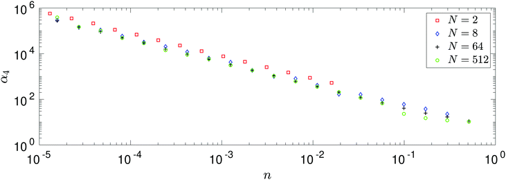
Calculating the number density in three spatial dimensions by n = N/L3, we can study the behaviour of kurtosis α4 as n varies. The results are presented in Fig. 4. We see general agreement between behaviour of each of the four systems. We see when n is equal, the values of kurtosis are larger for N = 2 than for the many-body systems with N = 8, 64, 512, which agree well amongst themselves.
 |
| | Fig. 4 Dependence of kurtosis α4 on density n. Each of the larger atomic systems (N = 8, 64, 512) is simulated over the same domain of number densities, while the N = 2 system is simulated in a sparser domain, though all are simulated in three spatial dimensions. We truncate the results of the N = 2 simulation in the plot, however the additional data points are used to calculate the results displayed in Fig. 5. | |
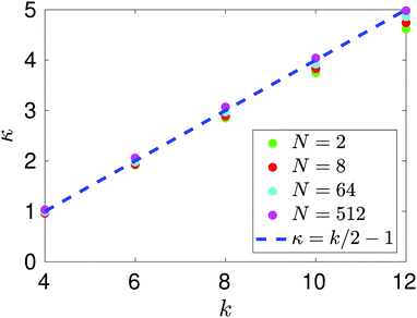
The results in Fig. 4 enable us to test the asymptotic expression (38) for k = 4 derived in the limit n → 0. Utilising similar log–log plots for MD data, we estimate the power law behaviour of each standardised moment, αk, for k = 4, 6, 8, 10, 12. Fig. 5 illustrates the results. All systems agree well with the predicted asymptotic behaviour (38), in particular the N = 512 atom system. There is a slight deviation between the results due to the fact that the smaller atom systems require a larger tsim in order to converge fully to the predicted value. This discrepancy is amplified when looking at higher standardised moments due to the fact that we are calculating statistics resulting from F121 (i.e. for α12) compared to F41 (i.e. for α4), for example.
 |
| | Fig. 5 Comparison of the results of MD simulations for a range of values of the number of atoms, N. After long time simulation, we compute the asymptotic behaviour αk ∝ n−κ and compare the leading order power scalings for each system. We compare this with the theoretical result (38) (denoted as a blue dashed line) that in the limit n → 0 we expect the universal behaviour κ = k/2 − 1, where k = 2, 4, 6,… denotes which standardised moment of force we are looking at. | |
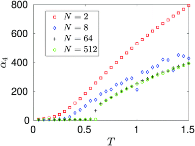
The dependence of kurtosis α4 on temperature T is presented in Fig. 6, where we keep the density fixed at n = n0 given in Table 1. We observe that as temperature increases so does the kurtosis of the force distribution associated with each system. This can be explained in terms of the dynamics of the interacting atom system. If we maintain each system in the canonical ensemble, we expect on average that each atom will have a kinetic energy equivalent to 3 T/2 (when in reduced units). As we increase this target temperature, the atoms become more energetic and thus are able to probe closer inter-atomic distances before a large repulsive force overcomes this inertial attraction. The range of forces on the tagged particle widens as temperature increases and therefore contributes to more outlier results in the distribution – leading to heavier tails and therefore distributions which become increasingly leptokurtic.
 |
| | Fig. 6 Dependence of kurtosis α4 on temperature T. Each atomic system is simulated at approximately the same density n = n0 given in Table 1. | |
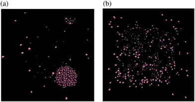
In Fig. 6, we observe that there is a qualitative difference between the results for N = 2 and larger atom systems. We see a bifurcation for the N = 64 and N = 512 systems at some temperature T* ∈ (0.6, 0.65), where a steady increase in kurtosis changes to a rapid increase. This bifurcation point in the phase plane lies on the coexistence boundary with (n, T) = (1/64, T*) and is due to a clustering mechanism which has been seen in MD simulations of Lennard-Jones fluids.29 From our results we see that the N = 2 system has missed this behaviour completely. Snapshots of the N = 512-atom system at some T = 0.6 < T*, and T = 0.66 > T* are displayed in Fig. 7. For T = 0.6, we see a large cluster has formed in the many-atom system. There would be far fewer outlier force results in this case due to the fact that the large majority of atoms are moving as a collective and effectively have fixed inter-atomic forces. Compared to the T = 0.66 snapshot, where we see that the atoms are too kinetically unstable to form these larger stable cluster structures, this results in more outlier forces felt between atoms due to the fact that the system is intrinsically more disordered. It is useful to note that this bifurcation point is located on the vapour-liquid coexistence boundary, the mechanisms of which have been studied on dilute Lennard-Jones fluids;30 here we see that this results in a bifurcation on standardised moments of the force distribution.
 |
| | Fig. 7 Snapshots31 of the MD simulation are taken for the system with N = 512 atoms at time t = 7.5 × 10⁵ for: (a) T = 0.6 < T*; and (b) T = 0.66 > T*. Density is n = 1/64. | |
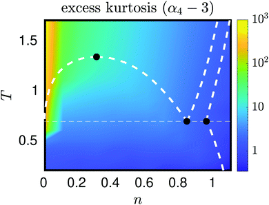
To understand the underlying variations of kurtosis, α4, with respect to changes in temperature and density, we use 12 × 16 MD simulations with N = 512 atoms and tsim = 3 × 10⁶, varying simulation parameters (n, T), where n = 10−2 + (i − 1)/10, for i = 1, 2,…, 12, and T = 10−1 + j/10, for j = 1, 2,…, 16. The sampled values of kurtosis, pressure and internal energy are included in the ESI.† The results for excess kurtosis (α4 − 3) are displayed in Fig. 8. Here a bifurcation can be seen when using the smallest density n = 0.01, as the change in colour is prominent in this vertical strip, indicating a large change of kurtosis. This occurs around T = 0.6, which is consistent with the result in Fig. 6, where we saw the bifurcation similarly located, though the slight shift in temperature is accounted for by the change in density parameters used in each simulation (namely n = 0.01 in Fig. 8 and n = 1/64 in Fig. 6).
 |
| | Fig. 8 The excess kurtosis, α4 − 3, calculated as a function of density n and temperature T for n ≤ 1.11 and T ≤ 1.7. The white dotted lines describe coexistence lines of different phases of a Lennard-Jones fluid taken from the literature.32–35 The solid black dots indicate (from left to right), the critical point and vapour–liquid–solid triple points. | |
In general, this low density strip contains the largest values of kurtosis, and covers much of the purely gas phase of the Lennard-Jones fluid. This paper has so far probed the low density limit in an attempt to understand why the standardised moments of force are so large, though Fig. 8 gives a good overview that in general, regardless of phase, a decrease in temperature, or an increase in density, systematically lead to a lower value of standardised moments. In this case as n → ∞ or T → 0, we expect the α4 → 3 (excess kurtosis tends to zero). This limiting regime corresponds to the solid phase of a Lennard-Jones system, where the force variations are minimal and the distribution is Gaussian. There is not enough space, nor energy, that lead to (many) outlier forces experienced by any atom, so the force distribution becomes less and less skewed from Gaussian, the deeper we probe in these regions. This intuition was demonstrated analytically in Section III.E when we showed this limiting behaviour on a 1D cartoon model with eqn (31). It is interesting to note that these changes in values of α4 appear smooth about changes in temperature and density (in absence of the bifurcation point for larger values of n), regardless of phase transitions.
V. Discussion and conclusions
In Section III we have demonstrated use of a variety of methods to study the standardised moments of the force distribution in order to probe both their temperature and number density dependence. This gave way to a rich structure where we show that the partition function for a 1D system can be calculated entirely from these standardised moments. Extending the far field method introduced in Section III.B to a system with N atoms in three-dimensional physical space, Section IV studies the dependence of αk on number density n, deriving the asymptotic expression (38). Our analytic results are contrasted with MD simulations of four systems of N = 2, 8, 64, 512 interacting Lennard-Jones atoms and these are compared. The results agree well with theoretical predictions though the results for systems with larger values of N are seen to converge more readily to the theoretically predicted results. In particular, rich dynamics such as clustering of Lennard-Jones fluids is completely missed by the systems with smaller values of N, but captured for systems with N as small as N = 64 atoms. In general, as temperature increases αk increases due to energetic nature of atoms allowing them to push closer together and experience larger forces. Clustering exhibited at the vapour–liquid coexistence phase incurs a bifurcation point whereby a large increase is seen in the standardised moments of force in Fig. 6, though a general increase in temperature, or decrease in number density, results in an increase in a4 regardless of the temperature/number density domain studied, as shown in Fig. 8.
Data availability
In compliance with EPSRC's open access initiative, the data in this paper is available from https://doi.org/10.5287/bodleian:GOMrMbXQe and in the ESI.†
Conflicts of interest
There are no conflicts of interest to declare.
Appendix A: constants Ck,1 and Ck,2 in eqn (29)
The constants appearing in eqn (29), namely Ck,1 and Ck,2, are given by formulas| |  | (A1) |
| |  | (A2) |
which can be derived in the following manner. Using Fk(r) = (U′(r))k for even values of k and U′(r*) = 0, we first note that
| Fk,k(r*) = k! (U′′(r*))k, |
| Fk,m(r*) = 0, for m ≤ k − 1, |
where Fk,m denotes the m-th derivative of Fk, i.e. the m-th derivative of the k-th power of F. Therefore, the first three non-zero terms of the Taylor expansion of Fk(r) around r = r* are| |  | (A3) |
Therefore, we have Ck,1 = Fk,(k+1)(r*)/(k + 1)! and Ck,2 = Fk,(k+2)(r*)/(k + 2)! and, to derive eqn (A1) and (A2), we need to express derivatives Fk,m(r*) for m = k + 1 and m = k + 2 in terms of derivatives of U(r) at r = r*. Using the product rule, the m-th derivative of Fk(r) can be, in general, written as a finite sum of the form| |  | (A4) |
where F(i)(r) is the i-th derivative of function F(r) and C(α0, α1,…, αm) are constants, many of them equal to zero. In fact, all terms in the expansion (A4) have multiplicities that sum to k, that is we can only sum over sequences satisfying| |  | (A5) |
and all terms in the expansion (A4) have m derivatives, that is, we have| |  | (A6) |
where αi ∈ {0, 1,…, k} for i = 0, 1, 2,…, m. Eqn (A6) is of the form of a finite Diophantine equation, which has no closed form for the number of solutions. In particular, simplifying eqn (A4) by solving eqn (A5) and (A6) is, in general, not possible. However, noting the specific property that F(r*) = 0 = U′(r*), we see that all terms that have α0 ≠ 0 will vanish when evaluated at this unique minimum r = r*. In particular, we will obtain relatively simple forms of the sum (A4) for m = k + 1 and m = k + 2 by considering eqn (A5) and (A6) with α0 = 0.
First, let us consider that m = k + 1. Using α0 = 0, there is only one solution of eqn (A5) and (A6) in non-negative integers, namely α1 = k − 1, α2 = 1 and α3 = α4 = … = 0. Therefore, eqn (A4) implies
| Fk,(k+1)(r*) = C(0, k − 1, 1, 0,⋯, 0) (F(1)(r*))k−1F(2)(r*). |
Using the general Leibniz rule,
36 we evaluate the combinatorial prefactor as
C(0,
k − 1, 1, 0,…, 0) =
k (
k + 1)! /2. Substituting into
Ck,1 =
Fk,(k+1)(
r*)/(
k + 1)! and using
F(
r*) = −
U′(
r*) and that
k is an even integer, we obtain formula (A1).
Second, we consider the case m = k + 2. Using α0 = 0, there are two solutions of eqn (A5) and (A6) in non-negative integers. The first solution is α1 = k − 1, α2 = 0, α3 = 1 and α4 = α5 = ⋯ = 0. The second solution is α1 = k − 2, α2 = 2 and α3 = α4 = ⋯ = 0. Therefore, eqn (A4) implies
Using the general Leibniz rule,
36 we evaluate these combinatorial prefactors as
Substituting into formula
Ck,2 =
Fk,(k+2)(
r*)/(
k + 2)! and using
F(
r*) = −
U′(
r*) and that
k is an even integer, we obtain eqn (A2). Thus, we have arrived at the expressions for
Ck,1 and
Ck,2 that are used in eqn (29).
Appendix B: thermostats used in MD simulations
Considering simulations presented in Fig. 2–6 and 8, we use a Nosé–Hoover thermostat. Its parameter, originally37 denoted Q, is the relaxation time of the thermostat. It is a measure of how strongly the thermostat is attached to the dynamics of the system. Its value for each simulation is given in the ESI.† In Fig. 6, we choose Q = 10T for each simulation; this linear scaling with T is necessary as we need to more tightly couple the thermostat at lower temperatures in order to accurately maintain the system in the canonical ensemble.38
For 1D simulations in Fig. 1, we maintain the canonical ensemble at a target (reduced) temperature T by implementing a Langevin thermostat. This is due to problems with ergodicity utilising the Nosé–Hoover thermostat for small systems,39,40 which can be seen in Fig. S3 in the ESI,† although the Nosé–Hoover thermostat ensures good temperature control for the average simulation temperature in Fig. S3 (ESI†). Fig. S4 in the ESI† highlights that the many body systems display ergodicity. With the Langevin dynamics for simulations in Fig. 1, the evolution of the free particle is modelled (in reduced units) as41,42
| |  | (B1) |
where
R(
t) is standard white noise and
γ = 0.1 acts as a friction parameter.
Acknowledgements
This work was supported by the Royal Society [grant number RGF\EA\180058] and by the Engineering and Physical Sciences Research Council [grant number EP/V047469/1].
References
- S. Joshi and S. Deshmukh, A review of advancements in coarse-grained molecular dynamics simulations, Mol. Simul., 2021, 47(10–11), 786–803 CrossRef CAS.
- Y. Wang,
et al., Effective force coarse-graining, Phys. Chem. Chem. Phys., 2009, 11, 2002 RSC.
-
R. Erban and S. J. Chapman, Stochastic modelling of reaction-diffusion processes, Cambridge Texts in Applied Mathematics, Cambridge University Press, 2020 Search PubMed.
- H. Ingólfsson,
et al., The power of coarse graining in biomolecular simulations, Wiley Interdiscip. Rev.: Comput. Mol. Sci., 2014, 4(3), 225 Search PubMed.
- A. Davtyan,
et al., Dynamic force matching: A method for constructing dynamical coarse-grained models with realistic time dependence, J. Chem. Phys., 2015, 142, 154104 CrossRef PubMed.
- R. Erban, Coupling all-atom molecular dynamics simulations of ions in water with Brownian dynamics, Proc. R. Soc. A, 2016, 472(2186), 20150556 CrossRef PubMed.
- D. Wales, Exploring energy landscapes, Annu. Rev. Phys. Chem., 2018, 69, 401 CrossRef CAS PubMed.
- R. Gunaratne,
et al., On short-range and long-range interactions in multi-resolution dimer models, Interface Focus, 2019, 9(3), 0070 CrossRef PubMed.
- E. Rolls, Y. Togashi and R. Erban, Varying the resolution of the Rouse model on temporal and spatial scales: Application to multiscale modelling of DNA dynamics, Multiscale Model. Simul., 2017, 15(4), 1672 CrossRef.
- R. Erban, From molecular dynamics to Brownian dynamics, Proc. R. Soc. A, 2014, 470(2167), 0036 CrossRef PubMed.
- L. DeCarlo, On the meaning and use of kurtosis, Psychol. Methods, 2014, 2(3), 292 Search PubMed.
- A. Carof, R. Vuilleumier and B. Rotenberg, Two algorithms to compute projected correlation functions in molecular dynamics simulations, J. Chem. Phys., 2014, 140, 124103 CrossRef PubMed.
- H. Shin,
et al., Brownian motion from molecular dynamics, Chem. Phys., 2010, 375, 316 CrossRef CAS.
- R. Erban, Coarse-graining molecular dynamics: Stochastic models with non-Gaussian force distributions, J. Math. Biol., 2020, 80, 457 CrossRef PubMed.
- S. Chandrasekhar, Stochastic problems in physics and astronomy, Rev. Mod. Phys., 1943, 15, 1 CrossRef.
- A. Gabrielli,
et al., Force distribution in a randomly perturbed lattice of identical atoms with 1/r2 pair interaction, Phys. Rev. E: Stat., Nonlinear, Soft Matter Phys., 2006, 74, 021110 CrossRef PubMed.
- G. Rickayzen,
et al., Single atom force distributions in simple fluids, J. Chem. Phys., 2012, 137, 094505 CrossRef CAS PubMed.
- A. C. Branka, D. M. Heyes and G. Rickayzen, Pair force distributions in simple fluids, J. Chem. Phys., 2011, 135, 164507 CrossRef CAS PubMed.
- J. Jones, On the determination of molecular fields. II. From the equation of state of a gas, Proc. R. Soc. A, 1924, 106, 738 Search PubMed.
- H. Watanabe, N. Ito and C. Hu, Phase diagram and universality of the Lennard-Jones gas-liquid system, J. Chem. Phys., 2012, 136, 204102 CrossRef PubMed.
- J.-P. Hansen and L. Verlet, Phase transitions of the Lennard-Jones system, Phys. Rev., 1969, 184, 151 CrossRef CAS.
- A. Rahman, Correlations in the motion of atoms in liquid argon, Phys. Rev. A: At., Mol., Opt. Phys., 1964, 136(2A), A405–A411 CrossRef.
- L. Verlet, Computer “experiments” on classical fluids. I. Thermodynamical properties of Lennard-Jones molecules, Phys. Rev., 1967, 159(1), 98–103 CrossRef CAS.
-
D. Frenkel and B. Smit. Understanding molecular simulation: From algorithms to applications, 2nd edn, Academic Press, 1996 Search PubMed.
- L. Rowley, D. Nicholson and N. G. Parsonage, Monte Carlo grand canonical ensemble calculation in a gas-liquid transition region for 12-6 Argon, J. Comput. Phys., 1975, 17, 401 CrossRef CAS.
-
D. Lide, Properties of the elements and inorganic compounds; melting, boiling, triple, and critical temperatures of the elements. CRC Handbook of Chemistry and Physics, 86th edn, CRC Press, 2005, ch. 4 Search PubMed.
- A. Giró, E. Guardia and J. A. Padró, Langevin and molecular dynamics simulations of Lennard-Jones liquids, J. Mol. Phys., 1985, 55(5), 1063–1074 CrossRef.
-
C. M. Bender and S. A. Orszag, Advanced mathematical methods for scientists and engineers: asymptotic methods and perturbation theory: v. 1, Springer, 1999 Search PubMed.
- N. Yoshii and S. Okazaki, Molecular dynamics study of structure of clusters in supercritical Lennard-Jones fluid, Fluid Phase Equilib., 1998, 144(1–2), 225 CrossRef CAS.
- J. Jung, J. Lee and J. Kim, Cluster growth mechanisms in Lennard-Jones fluids: a comparison between molecular dynamics and Brownian dynamics simulations, Chem. Phys., 2015, 449, 1 CrossRef CAS.
- W. Humphrey, A. Dalke and K. Schulten, VMD – visual molecular dynamics, J. Mol. Graph., 1996, 14, 33 CrossRef CAS PubMed.
- A. Schultz and D. Kofke, Erratum: “Comprehensive high-precision high-accuracy equation of state and coexistence properties for classical Lennard-Jones crystals and low-temperature fluid phases”, J. Chem. Phys., 2020, 153, 059901 CrossRef CAS PubMed.
- S. Stephan,
et al., Thermophysical properties of the Lennard-Jones fluid: database and data assessment, J. Chem. Inf. Model., 2019, 59(10), 4248 CrossRef CAS PubMed.
- S. Stephan, J. Staubach and H. Hasse, Review and comparison of equations of state for the Lennard-Jones fluid, Fluid Phase Equilib., 2020, 523, 112772 CrossRef CAS.
- E. Mastny and J. de Pablo, Melting line of the Lennard-Jones system, infinite size, and full potential, J. Chem. Phys., 2007, 127, 104504 CrossRef PubMed.
- A. Traheem and A. Laradji, Classroom note: A generalization of Leibniz rule for higher derivatives, Int. J. Math. Educ. Sci. Technol., 2003, 34(6), 905 CrossRef.
- S. Nosé, A molecular dynamics method for simulations in the canonical ensemble, Mol. Phys., 1984, 52(2), 255 CrossRef.
-
P. H. Hünenberger, Thermostat Algorithms for Molecular Dynamics Simulations, in Advanced Computer Simulation. Advances in Polymer Science, ed. C. Holm and K. Kremer, Springer, Berlin, Heidelberg, 2005, vol. 173, pp. 105–149 Search PubMed.
- M. E. Tuckerman,
et al., Non-Hamiltonian molecular dynamics: Generalizing Hamiltonian phase space principles to non-Hamiltonian systems, J. Chem. Phys., 2001, 115, 1678 CrossRef CAS.
- P. F. Tupper, Ergodicity and the numerical simulation of Hamiltonian systems, SIAM J. Appl. Dynam. Syst., 2005, 4(3), 563 CrossRef.
-
T. Schlick, Molecular modeling and simulation, Springer, 2002 Search PubMed.
-
B. Leimkuhler and C. Matthews, Molecular dynamics with deterministic and stochastic numerical methods, Springer Interdiscip. Appl. Math., 2015, vol. 39.
Footnote |
| † Electronic supplementary information (ESI) available. See DOI: 10.1039/d1cp04056a |
|
| This journal is © the Owner Societies 2022 |
Click here to see how this site uses Cookies. View our privacy policy here.  Open Access Article
 and
Radek
Erban
 *
*


![[Doublestruck R]](https://www.rsc.org/images/entities/char_e175.gif) 3 is given (in reduced units24) by the expression
3 is given (in reduced units24) by the expression
![[Doublestruck R]](https://www.rsc.org/images/entities/char_e175.gif) 6, were pi denotes the momentum of the i-th atom. We work in the canonical ensemble with temperature T; the partition function therefore becomes
6, were pi denotes the momentum of the i-th atom. We work in the canonical ensemble with temperature T; the partition function therefore becomes
![[Doublestruck R]](https://www.rsc.org/images/entities/char_e175.gif) 3N ×
3N × ![[Doublestruck R]](https://www.rsc.org/images/entities/char_e175.gif) 3N. This denotes the phase space of our system. For systems of interest Ωp ≡
3N. This denotes the phase space of our system. For systems of interest Ωp ≡ ![[Doublestruck R]](https://www.rsc.org/images/entities/char_e175.gif) 3N. The underlying geometry of the system (and principle simulation cell) is a cubic box of size L > 0, therefore Ωq ≡ (−L/2, L/2] × … × (−L/2, L/2]. The phase space volume elements in eqn (4) are denoted by
3N. The underlying geometry of the system (and principle simulation cell) is a cubic box of size L > 0, therefore Ωq ≡ (−L/2, L/2] × … × (−L/2, L/2]. The phase space volume elements in eqn (4) are denoted by

![[Doublestruck R]](https://www.rsc.org/images/entities/char_e175.gif) 6N, normalised such that 〈1〉 = 1.
6N, normalised such that 〈1〉 = 1.
![[Doublestruck R]](https://www.rsc.org/images/entities/char_e175.gif) 3, for j = 2, 3,…, N, the total force F = [F1, F2, F3] on the tagged atom is
3, for j = 2, 3,…, N, the total force F = [F1, F2, F3] on the tagged atom is


![[thin space (1/6-em)]](https://www.rsc.org/images/entities/char_2009.gif) exp[−βU(L/2)] δL + O(δL2),
exp[−βU(L/2)] δL + O(δL2),


![[thin space (1/6-em)]](https://www.rsc.org/images/entities/char_2009.gif) exp[−βU(r)] has maxima when r = r* = 21/6 or when kU′′(r) = β(U′(r))2. This forms a cubic in r6 that can be solved. For the values of k used in this work, this sometimes results in a global maximum, that always lies at a distance less than r < r* from the origin. Therefore r* = 21/6 is the furthest maximum of the integrand from the origin.
exp[−βU(r)] has maxima when r = r* = 21/6 or when kU′′(r) = β(U′(r))2. This forms a cubic in r6 that can be solved. For the values of k used in this work, this sometimes results in a global maximum, that always lies at a distance less than r < r* from the origin. Therefore r* = 21/6 is the furthest maximum of the integrand from the origin.


![[scr Z, script letter Z]](https://www.rsc.org/images/entities/char_e14b.gif) 1(T, V). Considering L ≥ 10, the result is within 5% error when compared with the exact result (20), while for larger values of box width L the error decreases to around 1%, confirming that the formula (22) is valid in the asymptotic limit L → ∞.
1(T, V). Considering L ≥ 10, the result is within 5% error when compared with the exact result (20), while for larger values of box width L the error decreases to around 1%, confirming that the formula (22) is valid in the asymptotic limit L → ∞.

![[scr Z, script letter Z]](https://www.rsc.org/images/entities/char_e14b.gif) 1(T, V) obtained using the right hand side of eqn (22) with k = 4 and values of kurtosis (α4) estimated from MD simulation (blue dashed line). The exact values obtained by eqn (20) are plotted as the red dots.
1(T, V) obtained using the right hand side of eqn (22) with k = 4 and values of kurtosis (α4) estimated from MD simulation (blue dashed line). The exact values obtained by eqn (20) are plotted as the red dots.


![[thin space (1/6-em)]](https://www.rsc.org/images/entities/char_2009.gif)
![[scr Z, script letter Z]](https://www.rsc.org/images/entities/char_e14b.gif) 1) is equal to the average energy of the system, 〈E〉, we have
1) is equal to the average energy of the system, 〈E〉, we have
![[thin space (1/6-em)]](https://www.rsc.org/images/entities/char_2009.gif) f0)/∂T. Thus, using eqn (6), we confirm that the second term on the right hand side of eqn (26) is the average potential energy.
f0)/∂T. Thus, using eqn (6), we confirm that the second term on the right hand side of eqn (26) is the average potential energy.


![[Doublestruck R]](https://www.rsc.org/images/entities/char_e175.gif) 3 is denoted by rij = |qi − qj|. Taking into account the periodic boundary conditions, the distance |qi − qj| is the minimum image inter-atomic distance given by
3 is denoted by rij = |qi − qj|. Taking into account the periodic boundary conditions, the distance |qi − qj| is the minimum image inter-atomic distance given by
![[small xi, Greek, macron]](https://www.rsc.org/images/entities/char_e0cf.gif) = ζ−L [ζ/L] for ζ ∈
= ζ−L [ζ/L] for ζ ∈ ![[Doublestruck R]](https://www.rsc.org/images/entities/char_e175.gif) and [·] rounds a real number to the nearest integer. For an interacting N-body system the dimensionality of the integral given by eqn (7) is 3N. We first present an illustrative calculation with N = 2 interacting atoms in Section IV.A and then we study systems with larger values of N in Section IV.B.
and [·] rounds a real number to the nearest integer. For an interacting N-body system the dimensionality of the integral given by eqn (7) is 3N. We first present an illustrative calculation with N = 2 interacting atoms in Section IV.A and then we study systems with larger values of N in Section IV.B.

![[small script l]](https://www.rsc.org/images/entities/char_e146.gif) = q
= q![[small script l]](https://www.rsc.org/images/entities/char_e146.gif) 1 − q
1 − q![[small script l]](https://www.rsc.org/images/entities/char_e146.gif) 2 and η
2 and η![[small script l]](https://www.rsc.org/images/entities/char_e146.gif) = q
= q![[small script l]](https://www.rsc.org/images/entities/char_e146.gif) 1 + q
1 + q![[small script l]](https://www.rsc.org/images/entities/char_e146.gif) 2 for
2 for ![[small script l]](https://www.rsc.org/images/entities/char_e146.gif) = x, y, z. We note that r12 is only dependent on the ξ
= x, y, z. We note that r12 is only dependent on the ξ![[small script l]](https://www.rsc.org/images/entities/char_e146.gif) variables, therefore one can trivially integrate (33) through the η
variables, therefore one can trivially integrate (33) through the η![[small script l]](https://www.rsc.org/images/entities/char_e146.gif) variables as the integrand has no dependence on these to obtain
variables as the integrand has no dependence on these to obtain

![[thin space (1/6-em)]](https://www.rsc.org/images/entities/char_2009.gif) N
N![[thin space (1/6-em)]](https://www.rsc.org/images/entities/char_2009.gif) tsim/Δt data points. This is equal to 6 × 10¹¹ (resp. 1.536 × 10⁹) data points in the simulation with N = 2 (resp. N = 512) atoms.
tsim/Δt data points. This is equal to 6 × 10¹¹ (resp. 1.536 × 10⁹) data points in the simulation with N = 2 (resp. N = 512) atoms.