Nanoscale chemical characterization of a post-consumer recycled polyolefin blend using tapping mode AFM-IR

Abstract

The routine analysis of polymer blends at the nanoscale is usually carried out using electron microscopy techniques such as scanning electron microscopy (SEM) and transmission electron microscopy (TEM), which often require several sample preparation steps including staining with heavy metals and/or etching. Atomic force microscopy (AFM) is also commonly used, but provides no direct chemical information about the samples analyzed. AFM-IR, a recent technique which combines the AFM's nanoscale resolution with the chemical information provided by IR spectroscopy, is a valuable complement to the already established techniques. Resonance enhanced AFM-IR (contact mode) is the most commonly used measurement mode, due to its signal enhancement and relative ease of use. However, it has severe drawbacks when used in highly heterogenous samples with changing mechanical properties, such as polymer recyclates. In this work, we use the recently developed tapping mode AFM-IR to chemically image the distribution of rubber in a real-world commercially available polyethylene/polypropylene (PE/PP) recycled blend derived from municipal and household waste. Furthermore, the outstanding IR resolution of AFM-IR allowed for the detection of small PP droplets inside the PE phase. The presence of micro and nanoscale particles of other polymers in the blend was also established, and the polymers identified.

---

Introduction

Plastic waste and its improper disposal are environmental hazards whose consequences are visible, but not yet fully understood (ex. effect of microplastic contamination).^1–5 As the production of polymer materials is increasing, and both long term storage in landfills and incineration are wasteful and hazardous to the environment, only plastic production from polymer waste (recycling) can reduce plastic waste.^6,7 However, waste plastics can contain contaminants or additives from their “previous lives” that can hinder the recycling process and lead to lower quality products when compared to virgin plastics.^8–10 For example, the presence of other polymer types in the final blend can lead to a degradation of the mechanical properties, especially when these are immiscible.¹¹ This can be particularly challenging when managing originally heterogeneous feedstock, made of different polymers. Furthermore, the better the sorting of shredded plastics, the higher the cost of recycling, and this approach may be inefficient in cases like multilayer packaging¹² or even in the case of homogeneous plastic waste which is mixed together during waste collection.^13,14 Therefore, heterogeneous recyclates that retain desirable mechanical properties may have a cost advantage over other single-polyolefin recyclates in similar applications due to the minimal sorting required.¹⁵

Polyethylene (PE) and isotactic polypropylene (PP) are two polyolefins that are immiscible with each other despite their structural similarity, and whose blend morphology varies with the blend composition.¹⁶ PE/PP blends generally suffer from low interfacial adhesion and the resulting mechanical properties make them unsuitable for higher value applications.^17,18 Several compatibilizers have been tested to improve the miscibility of PE and PP, and a comprehensive review can be found in literature.¹⁹ These include ethylene propylene rubber (EPR), ethylene propylene diene monomer rubber (EPDM), and styrene-b-(ethylene-co-butylene)-b-styrene (SEBS).^20–22 Common methods employed to analyse a polymer's micro- and nano-scale morphologies are scanning electron microscopy (SEM), transmission electron microscopy (TEM), and fluorescence confocal microscopy.^13,20,23 These methods have some disadvantages such as extra sample preparation steps (chemical etching, staining with heavy metals) in the case of electron microscopy or the need to label with fluorescent molecules in the case of confocal fluorescence microscopy.^13,20,23 Furthermore, all of the previously mentioned studies used either virgin polymer blends prepared specifically for the study, or blends where only the PE and PP components came from a waste stream, thus reducing the uncertainty of composition associated with fully recycled blends.

However, when the composition of recyclates is uncertain, established staining protocols might not be enough to fully understand the phase composition at the nanoscale. Here, AFM-IR (also known as photothermal infrared spectroscopy (PTIR)) provides an alternative approach towards the morphology characterization of recycled polymer blends. AFM-IR is a near-field technique that provides chemical identification via IR spectroscopy at lateral resolutions as small as ≈10 nm in tapping mode.²⁴ This resolution is achieved because the signal detection occurs in the near-field, and is thus not diffraction limited. In AFM-IR, the thermal expansion of the sample caused by the absorption of radiation from a pulsed wavelength-tunable IR laser is detected by the AFM tip, and it is proportional to the absorbed energy.²⁵ As is the case in bulk infrared spectroscopy, the AFM-IR signal is proportional to the wavelength-dependent absorption coefficient,²⁵ meaning that AFM-IR benefits from the long established spectra-structure correlations known to infrared spectroscopy. AFM-IR has found applications in geology,^26,27 environmental analysis,^28,29 material,^30,31 and life sciences.^32–35

Previous AFM-IR studies on the morphology of virgin high-impact PP and virgin PP/PE/EPR blends were carried out using contact-mode AFM-IR.^36–39 In contact mode AFM-IR – specifically the more sensitive “resonance enhanced” implementation – the laser repetition rate is set to match a mechanical contact resonance of the cantilever, which leads to an enhancement of the signal when compared to the older ring-down mode.⁴⁰ In this reliance on contact resonances lies also one of the down-sides of resonance enhanced measurements, particularly during imaging: local changes in the sample's mechanical properties lead to changes in the resonance frequency, which in turn leads to changes in the signal amplitude. To circumvent this problem, the measurement is either conducted off resonance (forgoing the resonant enhancement),⁴¹ by chirping the laser repetition within a likely range of the resonance (i.e. trading some sensitivity for accurate tracking of the resonance),⁴² or with the help of a phase locked loop (PLL) that tracks the changes in resonance frequency and adjusts the driving frequency/laser repetition rate accordingly.⁴²

It has long been recognized that tapping mode AFM, i.e. a mode where the AFM tip is driven to oscillation and the tip oscillation amplitude is used as feedback for the cantilever sample distance, is more adept than contact mode AFM for the analysis of soft materials (such as polymers).^43–45 Tapping mode AFM eliminates lateral tip-sample forces which can damage or deform the sample and the high vertical speed of the tapping tip leads to an increased apparent stiffness of viscoelastic samples.^46,47

Like resonance enhanced AFM-IR, the recently introduced tapping mode AFM-IR,⁴⁸ also relies on mechanical resonance for signal enhancement, but in tapping mode the resonance frequency of the cantilever is less sensitive to changes in the sample's mechanical properties.^49,50 This means there is no need to track the resonance frequency, thus reducing the complexity of the experiment. Additionally, tapping mode has a better resolution than contact mode (10 nm vs. 20 nm), due to the reduced interaction time between the tip and the sample.⁵⁰ For these reasons, tapping mode AFM-IR is better suited for the analysis of heterogeneous polymer samples with unpredictable changes in mechanical properties. Since this technique is still relatively recent, there are, to the best of our knowledge, no published tapping mode AFM-IR studies on polymers, with the exception of a protocol recently developed by our group.⁵¹ In this work, we go beyond the straightforward application of tapping mode AFM-IR to a polyolefin material by using tapping mode AFM-IR to study the phase distribution and the interphase between PE/PP in a commercially available PE/PP recyclate blend. The analysed sample derives from a post-consumer waste stream containing PE, PP, and a rubber component. Thus, in contrast to previous investigations of polymer interfaces using AFM-IR, we are not studying a tightly controlled material made specifically for AFM-IR analysis but a real-world sample that contains variations in composition as well as an unknown amount of contaminants and fillers. Using tapping mode AFM-IR for recording spectra and images, and chemometric models for data analysis, we are able to locate the rubber component at the interface of the PE and PP and to detect the presence of other polymer contaminants. The AFM-IR data obtained through spectra and chemical images are in agreement with each other, and with data obtained from conventional methods (SEM and soluble fraction analysis), thus demonstrating that AFM-IR is a valuable tool for the nanoscale analysis of recycled polymer blends.

Experimental

Materials

The material studied in this work is a polyolefin mix recyclate, originating from pre-sorted municipal and household waste, and mechanically recycled. Given the origin of the feedstock used to produce this material, market average content of additional components (e.g. EPR rubber, fillers, additives) is to be expected.

SEM measurements

Samples were imaged with a ThermoFischer Apreo 2 SEM after RuO₄ staining. The specimen was first cut under cryo-conditions (−100 °C) using an ultra-cryo-microtome Leica EM-UC7. RuO₄ was produced during the staining procedure by mixing RuCl₃ with an aqueous solution of NaIO₄. A staining time of 6 hours at room temperature was used. To remove over-stained material, a second microtome cutting was performed.

Soluble fraction analysis

The crystalline (CF) and soluble fractions (SF) as well as the comonomer content of the respective fractions were measured by Crystex (crystallisation extraction) method on a Polymer Char Crystex 42 instrument as described in literature.⁵²

Sample preparation for AFM-IR

The samples were ultra-cryomicrotomed at −100 °C on a Leica EM-UC7 equipped with a Leica EM FC7 cryochamber and the resulting sections were placed on ZnS substrates (13 mm diameter × 1 mm thickness from Crystran).

AFM-IR measurements

All AFM-IR measurements were carried out using a Bruker nano-IR 3s coupled to a MIRcat-QT external cavity quantum cascade laser array (EC-QCL) from Daylight Solutions. Spectra covering the range from 910 cm⁻¹ to 1950 cm⁻¹ were obtained using AFM-IR in tapping mode with a heterodyne detection scheme. The measurements were obtained while driving the cantilever at its second resonance frequency (f₂ ≈ 1500 kHz) and demodulating the AFM-IR signal at the first resonance frequency (f₁ ≈ 250 kHz) using a digital lock-in amplifier (MFLI, Zurich Instruments). The laser repetition rate was set to f_L = f₂ − f₁ ≈ 1300 kHz. The cantilevers used were gold coated with nominal first free resonance frequencies of 300 ± 100 kHz and a nominal spring constant between 20 and 75 N m⁻¹ (Tap300GB-G from BudgetSensors). The laser source operated at 10% duty cycle and emitted laser pulses of up to 500 mW peak pulse power. Using metal mesh attenuators, the laser power was adjusted to between 39.66% and 49.6% of the original power (before beam splitter, nominal splitting ratio 1 : 1). For each location, 3 spectra were recorded at 1 cm⁻¹ spectral resolution. The instrument and all beam paths were purged with dry air generated by an adsorptive dry air generator.

Data pre-processing

Recorded AFM-IR spectra were averaged by location, normalized individually to the unit norm in the range between 1400 cm⁻¹ and 1500 cm⁻¹ and smoothed using a Savitzky–Golay filter (9 points, first order).

The shift between chemical images was corrected using sub pixel registration via phase cross correlation based on their simultaneously recorded topography counterparts as reference. Calculations were performed using the phase cross correlation implementation in the scikit-image package (v0.18.1) for Python 3.⁵³

Chemometric analysis

Modelling was performed using the scikit-learn (v0.24.2) machine learning library for Python 3.⁵⁴

The averaged and smoothed spectra were clustered using an agglomerative clustering model with 3 clusters.

The analysis of the chemical images was performed using a Gaussian mixture model with 3 components and 5 iterations.

Results & discussion

The post-consumer polyolefin mix recyclate derived from municipal waste investigated in this study was analyzed using soluble fraction analysis, AFM-IR, SEM, and AM–FM AFM.

Bulk characterization of the material was carried out by soluble fraction analysis (results shown in Table 1). The soluble fraction analysis used in this study allows for the determination of the amorphous content and for the analysis of the ethylene content in each of the obtained fractions.⁵² The soluble fraction (Table 1) corresponds mostly to the rubber content present in the sample (amorphous content), which has a total ethylene (C2) content of 46.6%. This fraction could correspond to the rubber compatibilizers EPR, EPDM, or SEBS which are expected to be present at the interface between the PE and PP phases, but further analysis is required to determine which one of them is present in our recyclate.

Table 1 Soluble fraction analysis of the material used in this study

SF (%wt)^a	C2 total (%wt)^b	C2 in SF (%wt)^c	C2 in CF (%wt)^d
a Soluble fraction. b Total ethylene content. c Ethylene content in the soluble fraction. d Ethylene content in the insoluble fraction.
8.5	47.6	46.6	48.4

---

The first AFM-IR measurements were collected from a 10 μm × 10 μm area of a sample section obtained through cryo-microtomy. After an analysis of full AFM-IR spectra obtained, images using tapping mode AFM-IR were recorded at 1377 cm⁻¹, 1462 cm⁻¹, 1640 cm⁻¹, and 1724 cm⁻¹. The spectrum of PE in the region from 950 cm⁻¹ to 1950 cm⁻¹ is dominated by the strong band at around 1468 cm⁻¹ corresponding primarily to the scissor bending of the CH₂ groups.⁵⁵ In the case of PP, in addition to the CH₂ scissor band at 1458 cm⁻¹ with contributions from the CH₃ asymmetric deformation vibration, a strong band at 1378 cm⁻¹ that originates from the symmetric deformation of CH₃ groups is also present.⁵⁶ The images obtained were drift-corrected as described in literature,⁵¹ and the logarithm of the ratio of CH₃ (1377 cm⁻¹) and CH₂ (1462 cm⁻¹) was calculated and is shown in Fig. 1(b). The ratio of CH₃/CH₂ allows us to visualize the distribution of PE (white) and PP (purple) in the sample and reveals the presence of droplets inside the larger PE domains that are similar to the outer PP phase. This morphology is peculiar because, in a system with roughly 50%/50% content of PP and PE (Table 1), one would expect a co-continuous phase morphology, made of two distinct PE and PP phases. Instead, probably during the extrusion part of the mechanical recycling process, the two materials are made to mix very intimately and small domains of PP are present in the PE phase. This is a new finding, since the size of these domains is not accessible to conventional Fourier transform infrared spectroscopy (FTIR) microscopes. The existence of patches with different properties can be observed in standard AFM images, however it is not possible to link this observation to chemical information.

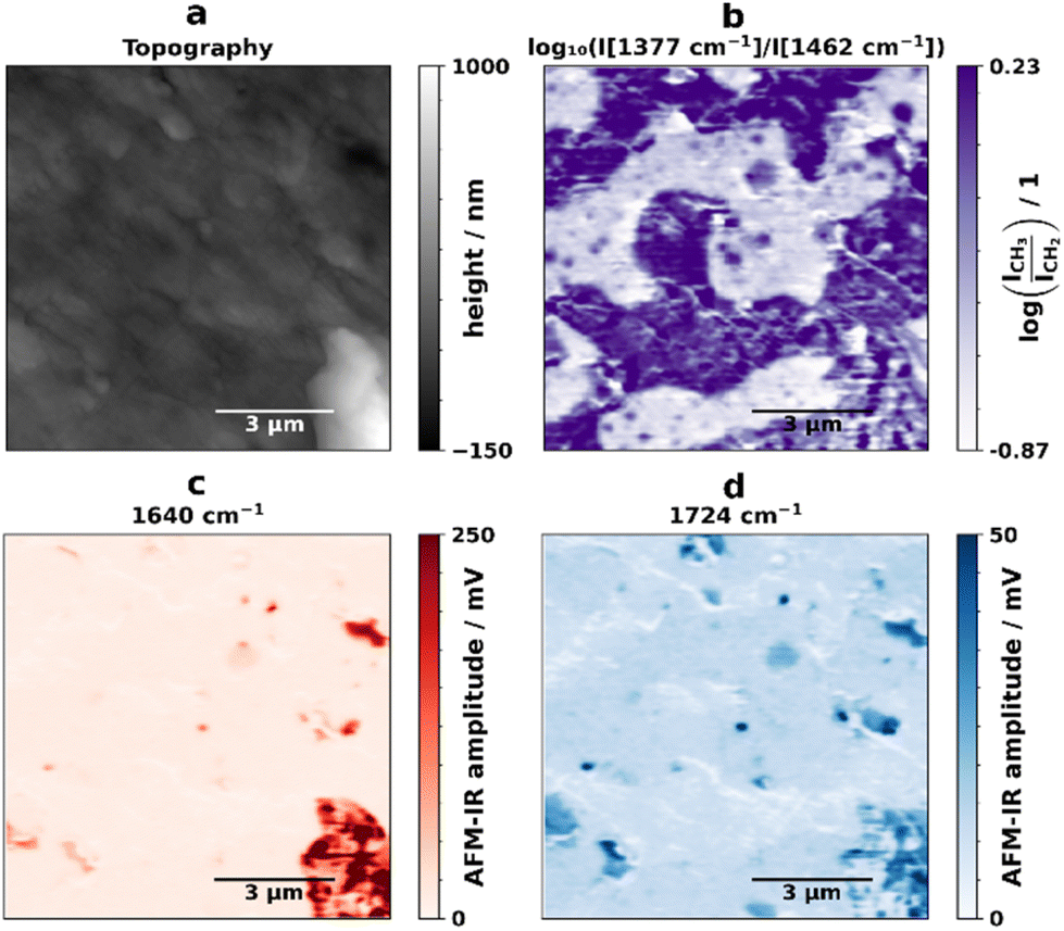Fig. 1 Topography (a) and chemical maps (10 × 10 μm). (b) Ratio of the bands corresponding to deformation vibrations of CH₂ (1462 cm⁻¹) and symmetric deformation of CH₃ groups (1377 cm⁻¹). (c) Chemical map obtained at 1640 cm⁻¹, corresponding to the distribution of polyamide. (d) Chemical map obtained at 1725 cm⁻¹, corresponding to the distribution of polyurethane.

Droplets of small size crystallize in a different fashion compared to the bulk material,⁵⁷ and therefore it is not yet known, what are the properties of these very small PP inclusions into the PE phase, or the implications they may have on e.g. mechanical properties. A previous study by Tang et al. had described the crystallization of PP-rich-sequences of EPR in the core–shell morphology of the rubber.³⁶ These findings differ from ours because not only was the material used different (commercially available recycled polyolefin mix vs. special grade high-impact poly-propylene), but also our results indicate that the small particles are PP and not just PP-rich sequences of EPR. This is supported by amplitude modulation–frequency modulation AM–FM AFM measurements (Fig. S1†) which reveal that the inclusions in the PE phase have the same Young's modulus as the PP matrix. If these particles were composed of PP-rich EPR sequences, then the Young's modulus should be lower, since these sequences would not crystalize as well as isotactic PP.⁵⁷

The images obtained at 1640 cm⁻¹ (Fig. 1(c), red) reveal the presence of several polyamide (PA) particles. The obtained full-length spectrum in an area with predominantly only 1640 cm⁻¹ (Fig. S2,† orange spectrum) is in accordance with FTIR spectra of PA found in literature.⁵⁸ The image at 1724 cm⁻¹ likely shows the presence of polyurethane (PU), since AFM-IR spectra obtained in an area with 1724 cm⁻¹ absorption but no 1640 cm⁻¹ absorption (see Fig. S2,† blue spectrum) show a band at 1602 cm⁻¹, as described in literature.⁵⁹ In some locations there is absorption at both 1640 cm⁻¹ and 1724 cm⁻¹. In this case it is not entirely clear whether this is due to the presence of polyurethane or degraded PA,⁶⁰ because the higher signal produced by the PA may be covering up the polyurethane 1602 cm⁻¹ signal, as indicated by the spectra in Fig. S2.† The PA and PU particles have sizes ranging from several microns to 200 nm (Fig. S3†). Information on the nature and size of contamination in recyclates is relevant, because the presence of other polymers that were not fully separated during the sorting process in the blend can be detrimental to the overall mechanical properties.⁶¹ Furthermore, it showcases the advantages of AFM-IR analysis as a technique that allows for the chemical identification of nano-scale impurities and their distribution in the analyzed samples without prior knowledge of said impurities.

To localize and identify the amorphous fraction detected in the soluble fraction analysis (Table 1), further AFM-IR images were collected in a smaller area of the same location (1.5 μm × 1.5 μm), which can be seen in Fig. 2, as well as full spectra in a grid format close to the interface and in a line over the PP inclusion (Fig. 3(a)). The CH₃/CH₂ ratio image (Fig. 2(b)) shows an intermediate color at the PP/PE interface, which hints at the presence of a component with intermediate ratio values, i.e. the rubber.

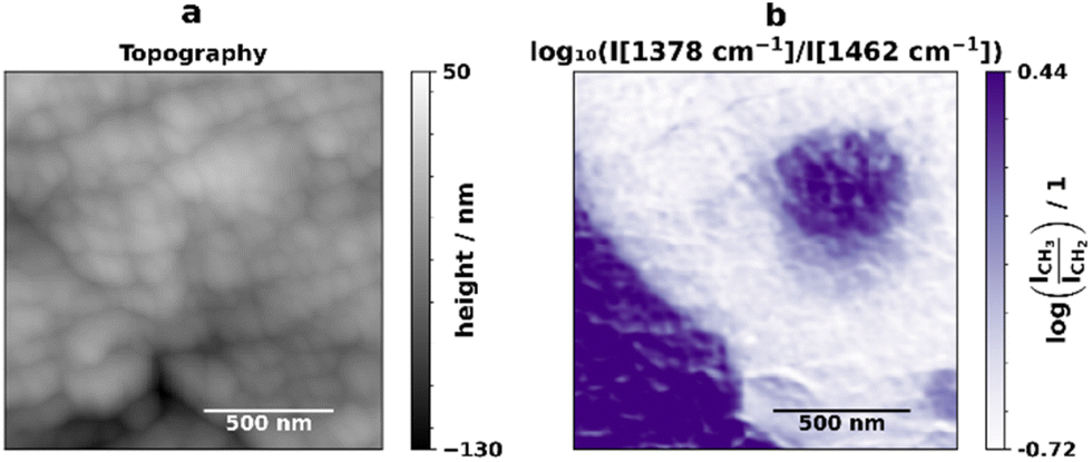Fig. 2 Topography (a) and band ratio (b) of the bands corresponding to deformation vibrations of CH₂ and symmetric deformation of CH₃ groups (1.5 μm × 1.5 μm).

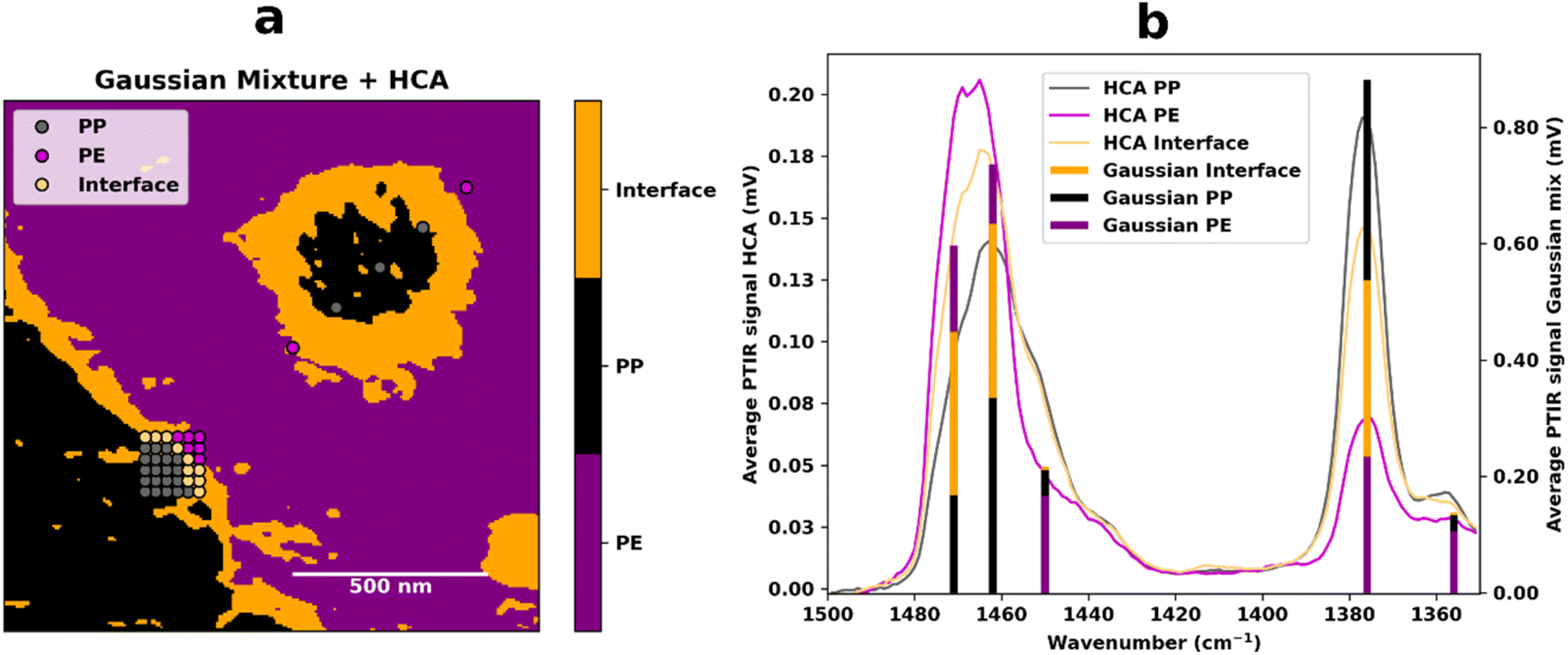Fig. 3 Results of the HCA and Gaussian mixture combined. (a) Gaussian mixture analysis on a 1.5 μm × 1.5 μm area and distribution of HCA clusters (each point corresponds to one full-length AFM-IR spectrum). (b) Average spectra of each HCA cluster (lines) and average value for each Gaussian mixture category (bars) plotted in the same graph for comparison.

However, to see the rubber interface, we need to combine information from more than just two wavelengths. To facilitate this task given the amount of data collected, two multivariate chemometric methods, hierarchical cluster analysis (HCA) and Gaussian mixture, were applied to the spectra and to the IR images respectively. For the analysis of the IR images, a Gaussian mixture model was chosen, since HCA is not optimal for the handling of large datasets due to its complexity (n is the number of samples). Fig. 3 shows the superposition of the Gaussian mixture image and the position of the spectral HCA clusters, as well as a combined plot of the average HCA cluster spectra and the average values of each Gaussian mixture subpopulation. The dendrogram obtained for the HCA is shown in Fig. S4.† The two different methods and ways of obtaining AFM-IR data are in agreement and support the hypothesis that the rubber is present at the interface. In the spectra, HCA clearly identifies the PP and PE components, as well as a third component (Fig. 3(a), yellow dots). This component has a band at 1378 cm⁻¹ (yellow) with an intermediate intensity compared to the correspondently higher PP (grey) and lower PE (pink) bands. The same trend is visible in the Gaussian mixture model (Fig. 3(b)). Here it is possible to once again see the distribution of PE and PP, which is in accordance with the ratio image (Fig. 2), and in addition to that, the distribution of the third component is now visible as well. As previously hinted at by the ratio image and the HCA, the rubber component is present at the interface and surrounds the PP droplets that are present inside the larger PE phase. The average values of each of the Gaussian mixture identified subpopulations show the same trends as the average spectra obtained for the HCA clusters.

The AFM-IR spectra taken at the interface (Fig. S5†) show no bands that can be assigned to aromatic rings, which would be expected in SEBS,⁶² hence we conclude that the material present at the interface is not SEBS. The two other major types of rubber compatibilizer, EPDM and EPR are hard to distinguish, since both have very similar IR spectra in the recorded range. A hint at the absence of EPDM is the lack of bands that could be assigned to unsaturated bonds, however the fraction of such bonds in EPDM would be low and might thus go undetected. Furthermore, due to EPR's abundance and relatively cheap cost, it is likely that the interface is composed of EPR, and not of the more expensive EPDM. Previous studies have found that the addition of EPR to a PE/PP blend leads to a finer phase dispersion and improves blend properties such as notched impact strength and ductility.²⁰ This is attributed to changes in the sub-micron scale, where the EPR forms a layer at the interface between the PE and PP with a core–shell-like morphology,^13,20,23 which is in agreement with our findings.

The results found in AFM-IR confirm those seen when applying an established protocol combining RuO₄ staining and SEM to highlight EPR content (see Fig. 4).²⁰ As observed in the AFM-IR data, SEM analysis confirms the presence of a brightly stained interface (rubber)⁶³ surrounding the PE (intermediate brightness) and PP (darker component) and also surrounding the PP droplets found inside some of the PE domains.

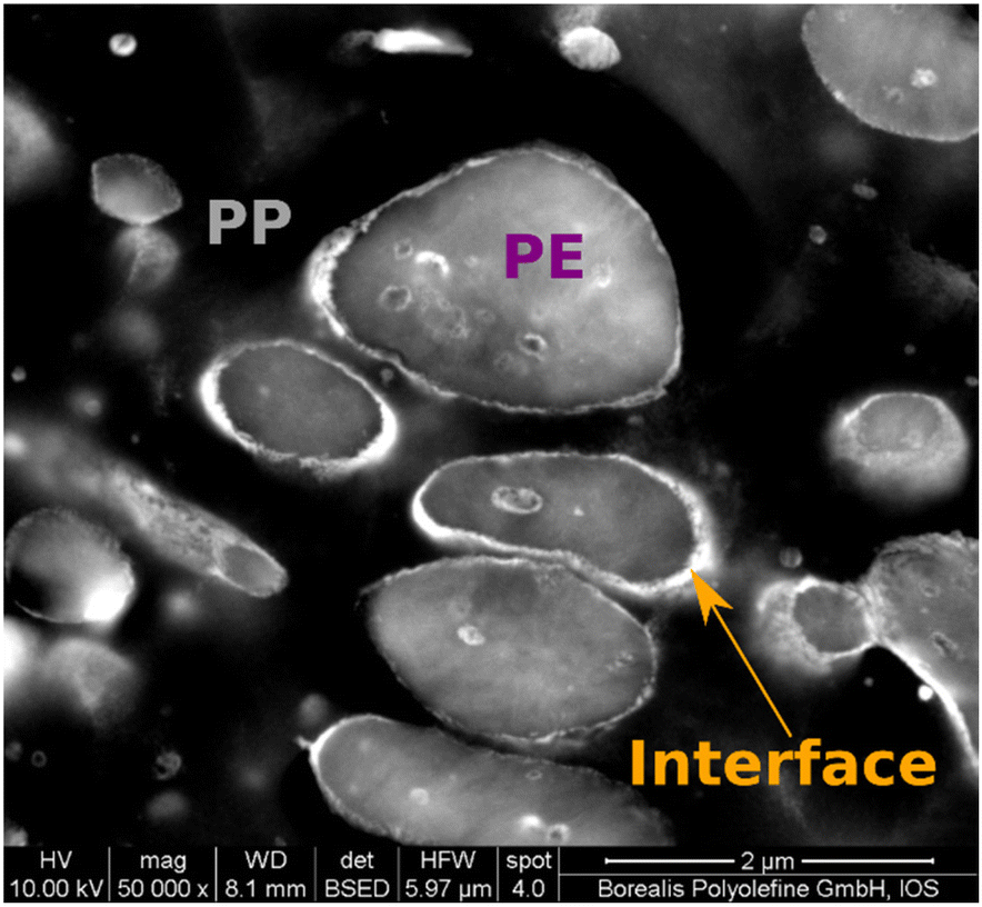Fig. 4 SEM image of the ruthenium-stained material used in this study. In ruthenium-stained SEM images amorphous polymers (such as rubber) appear brighter.⁶³

A previous contact mode AFM-IR study by Jiang et al.³⁸ on the interface of a PP/PE/EPR in-reactor alloy found that the EPR is present at the interface between PP and PE. In this study the lowest value of ethylene content (and thus highest value of PP chain segments) in the blend was found in a location at the interface between the PE core and EPR component. We do not see this type of arrangement in our sample, which is not surprising because the ethylene-propylene block copolymers (EbP) identified in Jiang et al.'s study are not commonly produced in industrial plants and require special catalysts.⁶⁴ Thus, it is not expected that a polyolefin recyclate that originates from household waste contains such special polymer grades.

Conclusions

This work constitutes the first use of tapping mode AFM-IR to perform a thorough study of the chemical composition and phase distribution of a real-world polyolefin recyclate at the nanoscale. This municipal waste derived (post-consumer) material is shown to contain the typical PP, PE phases and a rubber component. AFM-IR revealed the distribution of the rubber component at the interface of the PE and PP phases using its spectral signature without the need to staining of the sample. This result matches references measurements using SEM after staining with RuO₄ that rely on staining. The presence of small PP particles inside the larger PE phase that had previously been described for freshly prepared materials was also seen in the tapping mode AFM-IR analysis of this recycled polymer. However, in contrast to fresh polymers, in the studied recycled polymer the presence of non-polyolefine polymer inclusions was found. Here, the high sensitivity and spatial resolution of tapping mode AFM-IR is beneficial as it can detect particles orders of magnitude below the diffraction limit of conventional FTIR microscopy. All phases and contaminants were chemically identified using nanoscale spatial resolution mid-IR absorption spectra collected using the AFM-IR instrument. This constitutes a major advantage over established methods which indirectly identify phases via physical properties, or via staining or etching protocols. Hence, we expect a more widespread adoption of tapping mode AFM-IR in polymer nanoscale analysis in the near future.

Author contributions

A. Catarina V. D. dos Santos: conceptualization, investigation, formal analysis, visualization, writing – original draft; Davide Tranchida: conceptualization, resources, writing – review & editing; Bernhard Lendl: funding acquisition, resources, supervision, writing – review & editing; Georg Ramer: conceptualization, software, supervision, writing – review & editing.

Conflicts of interest

There are no conflicts to declare.

Acknowledgements

The authors would like to thank Walter Schaffer, Ljiljana Jeremic, Gottfried Kandioller, and Helmut Rinnerthaler from Borealis for sharing their expertise in polyolefin characterization.

The authors acknowledge financial support through the COMET Centre CHASE, funded within the COMET − Competence Centres for Excellent Technologies programme by the BMK, the BMDW and the Federal Provinces of Upper Austria and Vienna. The COMET programme is managed by the Austrian Research Promotion Agency (FFG). The authors acknowledge TU Wien Bibliothek for financial support through its Open Access Funding Programme.

Notes and references

1. L. Lebreton and A. Andrady, Palgrave Commun., 2019, 5, 1–11.
2. Q. Chen, J. Reisser, S. Cunsolo, C. Kwadijk, M. Kotterman, M. Proietti, B. Slat, F. F. Ferrari, A. Schwarz, A. Levivier, D. Yin, H. Hollert and A. A. Koelmans, Environ. Sci. Technol., 2018, 52, 446–456.
3. D. Santillo, K. Miller and P. Johnston, Integr. Environ. Assess. Manage., 2017, 13, 516–521.
4. E. Danopoulos, M. Twiddy and J. M. Rotchell, PLoS One, 2020, 15(7), e0236838.
5. E. Danopoulos, L. C. Jenner, M. Twiddy and J. M. Rotchell, Environ. Health Perspect., 2020, 128, 126002.
6. R. Geyer, J. R. Jambeck and K. L. Law, Sci. Adv., 2017, 3(7), e1700782.
7. M. Okan, H. M. Aydin and M. Barsbay, J. Chem. Technol. Biotechnol., 2019, 94, 8–21.
8. V. S. Cecon, P. F. Da Silva, G. W. Curtzwiler and K. L. Vorst, Resour., Conserv. Recycl., 2021, 167, 105422.
9. B. D. Vogt, K. K. Stokes and S. K. Kumar, ACS Appl. Polym. Mater., 2021, 3, 4325–4346.
10. M. K. Eriksen, K. Pivnenko, M. E. Olsson and T. F. Astrup, Waste Manage., 2018, 79, 595–606.
11. B. Hu, S. Serranti, N. Fraunholcz, F. Di Maio and G. Bonifazi, Waste Manage., 2013, 33, 574–584.
12. K. Kaiser, M. Schmid and M. Schlummer, Recycling, 2018, 3, 1.
13. M. Louizi, V. Massardier and P. Cassagnau, Macromol. Mater. Eng., 2014, 299, 674–688.
14. D. Wang, Y. Li, X.-M. Xie and B.-H. Guo, Polymer, 2011, 52, 191–200.
15. S. Billiet and S. R. Trenor, ACS Macro Lett., 2020, 9, 1376–1390.
16. I. Charfeddine, J. C. Majesté, C. Carrot and O. Lhost, Polymer, 2020, 193, 122334.
17. K. A. Chaffin, F. S. Bates, P. Brant and G. M. Brown, J. Polym. Sci., Part B: Polym. Phys., 2000, 38, 108–121.
18. B. C. Poon, S. P. Chum, A. Hiltner and E. Baer, Polymer, 2004, 45, 893–903.
19. A. Ghosh, Resour., Conserv. Recycl., 2021, 175, 105887.
20. G. Radonjič and N. Gubeljak, Macromol. Mater. Eng., 2002, 287, 122–132.
21. T. Kajiyama, T. Yasuda, T. Yamanaka, K. Shimizu, T. Shimizu, E. Takahashi, A. Ujiie, K. Yamamoto, T. Koike and Y. Nishitani, Int. Polym. Process., 2018, 33, 564–573.
22. N. V. Penava, V. Rek and I. F. Houra, J. Elastomers Plastics, 2013, 45, 391–403.
23. L. Li, L. Chen, P. Bruin and M. A. Winnik, J. Polym. Sci., Part B: Polym. Phys., 1997, 35, 979–991.
24. K. Wieland, G. Ramer, V. U. Weiss, G. Allmaier, B. Lendl and A. Centrone, Nano Res., 2019, 12, 197–203.
25. A. Dazzi, F. Glotin and R. Carminati, J. Appl. Phys., 2010, 107, 124519.
26. Y. Kebukawa, H. Kobayashi, N. Urayama, N. Baden, M. Kondo, M. E. Zolensky and K. Kobayashi, Proc. Natl. Acad. Sci. U. S. A., 2019, 116, 753.
27. K. Wang, L. Ma and K. G. Taylor, Fuel, 2022, 310, 122278.
28. V. W. Or, A. D. Estillore, A. V. Tivanski and V. H. Grassian, Analyst, 2018, 143, 2765–2774.
29. A. L. Bondy, R. M. Kirpes, R. L. Merzel, K. A. Pratt, M. M. Banaszak Holl and A. P. Ault, Anal. Chem., 2017, 89, 8594–8598.
30. T. Kong, H. Xie, Y. Zhang, J. Song, Y. Li, E. L. Lim, A. Hagfeldt and D. Bi, Adv. Energy Mater., 2021, 11, 2101018.
31. Y. Liu, L. Collins, R. Proksch, S. Kim, B. R. Watson, B. Doughty, T. R. Calhoun, M. Ahmadi, A. V. Ievlev, S. Jesse, S. T. Retterer, A. Belianinov, K. Xiao, J. Huang, B. G. Sumpter, S. V. Kalinin, B. Hu and O. S. Ovchinnikova, Nat. Mater., 2018, 17, 1013–1019.
32. R. Rebois, D. Onidas, C. Marcott, I. Noda and A. Dazzi, Anal. Bioanal. Chem., 2017, 409, 2353–2361.
33. D. Perez-Guaita, K. Kochan, M. Batty, C. Doerig, J. Garcia-Bustos, S. Espinoza, D. McNaughton, P. Heraud and B. R. Wood, Anal. Chem., 2018, 90, 3140–3148.
34. A. C. V. D. dos Santos, R. Heydenreich, C. Derntl, A. R. Mach-Aigner, R. L. Mach, G. Ramer and B. Lendl, Anal. Chem., 2020, 92, 15719–15725.
35. A. Deniset-Besseau, C. B. Prater, M.-J. Virolle and A. Dazzi, J. Phys. Chem. Lett., 2014, 5, 654–658.
36. F. Tang, P. Bao, A. Roy, Y. Wang and Z. Su, Polymer, 2018, 142, 155–163.
37. F. Tang, P. Bao and Z. Su, Anal. Chem., 2016, 88, 4926–4930.
38. C. Jiang, B. Jiang, Y. Yang, Z. Huang, Z. Liao, J. Sun, J. Wang and Y. Yang, Polymer, 2021, 214, 123373.
39. C. Li, Z. Wang, W. Liu, X. Ji and Z. Su, Macromolecules, 2020, 53, 2686–2693.
40. F. Lu and M. A. Belkin, Opt. Express, 2011, 19, 19942–19947.
41. S. Kenkel, A. Mittal, S. Mittal and R. Bhargava, Anal. Chem., 2018, 90, 8845–8855.
42. G. Ramer, F. Reisenbauer, B. Steindl, W. Tomischko and B. Lendl, Appl. Spectrosc., 2017, 71, 2013–2020.
43. S. N. Magonov and D. H. Reneker, Annu. Rev. Mater. Sci., 1997, 27, 175–222.
44. M. A. S. R. Saadi, B. Uluutku, C. H. Parvini and S. D. Solares, Surf. Topogr.: Metrol. Prop., 2020, 8, 045004.
45. G.-L. Liu and S. G. Kazarian, Analyst, 2022, 147, 1777–1797.
46. C. A. Putman, K. O. van der Werf, B. G. de Grooth, N. F. van Hulst and J. Greve, Biophys. J., 1994, 67, 1749–1753.
47. V. V. Tsukruk, V. V. Gorbunov, Z. Huang and S. A. Chizhik, Polym. Int., 2000, 49, 441–444.
48. M. Tuteja, M. Kang, C. Leal and A. Centrone, Analyst, 2018, 143, 3808–3813.
49. J. Mathurin, A. Deniset-Besseau and A. Dazzi, Acta Phys. Pol., A, 2020, 137, 29–32.
50. D. Kurouski, A. Dazzi, R. Zenobi and A. Centrone, Chem. Soc. Rev., 2020, 49, 3315–3347.
51. A. C. V. D. dos Santos, B. Lendl and G. Ramer, Polym. Test., 2022, 106, 107443.
52. L. Jeremic, A. Albrecht, M. Sandholzer and M. Gahleitner, Int. J. Polym. Anal. Charact., 2020, 25, 581–596.
53. S. van der Walt, J. L. Schönberger, J. Nunez-Iglesias, F. Boulogne, J. D. Warner, N. Yager, E. Gouillart, T. Yu and the scikit-image contributors, PeerJ, 2014, 2, e453.
54. F. Pedregosa, G. Varoquaux, A. Gramfort, V. Michel, B. Thirion, O. Grisel, M. Blondel, P. Prettenhofer, R. Weiss, V. Dubourg, J. Vanderplas, A. Passos, D. Cournapeau, M. Brucher, M. Perrot and É. Duchesnay, J. Mach. Learn. Res., 2011, 12, 2825–2830.
55. M. G. Olayo, E. Colín, G. J. Cruz, J. Morales and R. Olayo, Eur. Phys. J.: Appl. Phys., 2009, 48, 30501.
56. I. Prabowo, J. N. Pratama and M. Chalid, IOP Conf. Ser.: Mater. Sci. Eng., 2017, 223, 012020.
57. R. M. Michell, I. Blaszczyk-Lezak, C. Mijangos and A. J. Müller, Polymer, 2013, 54, 4059–4077.
58. J. C. Farias-Aguilar, M. J. Ramírez-Moreno, L. Téllez-Jurado and H. Balmori-Ramírez, Mater. Lett., 2014, 136, 388–392.
59. S. J. McCarthy, G. F. Meijs, N. Mitchell, P. A. Gunatillake, G. Heath, A. Brandwood and K. Schindhelm, Biomaterials, 1997, 18, 1387–1409.
60. E. S. Gonçalves, L. Poulsen and P. R. Ogilby, Polym. Degrad. Stab., 2007, 92, 1977–1985.
61. A. Schweighuber, M. Gall, J. Fischer, Y. Liu, H. Braun and W. Buchberger, Anal. Bioanal. Chem., 2021, 413, 1091–1098.
62. M. A. Vargas, N. N. López, M. J. Cruz, F. Calderas and O. Manero, Rubber Chem. Technol., 2009, 82, 244–270.
63. H. Sano, T. Usami and H. Nakagawa, Polymer, 1986, 27, 1497–1504.
64. J. M. Eagan, J. Xu, R. Di Girolamo, C. M. Thurber, C. W. Macosko, A. M. LaPointe, F. S. Bates and G. W. Coates, Science, 2017, 355, 814–816.

---

Footnote

† Electronic supplementary information (ESI) available: AM–FM AFM images, AFM-IR spectra, dendrogram and raw data. See DOI: https://doi.org/10.1039/d2an00823h

---