Unravelling the mechanism of glucose binding in a protein-based fluorescence probe: molecular dynamics simulation with a tailor-made charge model

Abstract

Fluorophores linked to the glucose/galactose-binding protein (GGBP) are a promising class of glucose sensors with potential application in medical devices for diabetes patients. Several different fluorophores at different positions in the protein were tested experimentally so far, but a deeper molecular understanding of their function is still missing. In this work, we use molecular dynamics simulations to investigate the mechanism of glucose binding in the GGBP-Badan triple mutant and make a comparison to the GGBP wild-type protein. The aim is to achieve a detailed molecular understanding of changes in the glucose binding site due to the mutations and their effect on glucose binding. Free simulations give an insight into the changes of the hydrogen-bonding network in the active site and into the mechanisms of glucose binding. Additionally, metadynamics simulations for wild type and mutant unravel the energetics of binding/unbinding in these proteins. Computed free energies for the opening of the binding pocket for the wild-type and the mutant agree well with the experimental data. Further, the simulations also give an insight into the changes of the chromophore conformations upon glucose binding, which can help to understand fluorescence changes. Therefore, the molecular details unravelled in this work may support effective optimisation strategies for the construction of more efficient glucose sensors.

---

1 Introduction

Effective diabetes treatment requires monitoring the patient's blood glucose concentration in real-time. However, the traditional finger-prick method cannot realise this real-time continuous glucose monitoring (CGM). On the other hand, the currently available sensors for CGM are facing limitations in accuracy and show a short service time. Hence, studies on developing new generations of CGM sensors are not only meaningful but also urgent.

Bacterial periplasmic glucose/galactose binding proteins (GGBP) of the Gram negative bacteria E. coli¹ and S. typhimorium² are promising tools for glucose recognition and have been commonly used as receptors in recent years. The probe consists of GGBP with an environmentally sensitive fluorophore attached at a specific position. This position is chosen such that a conformational change of the protein upon glucose binding leads to a significant fluorescence change due to a changed fluorophore environment. The important features of such probes are the magnitude of fluorescence change upon glucose binding, as well as the operating range of glucose concentration. This operating range is related to the binding strength as quantified by the dissociation constant (k_D).

Sensors of this kind were firstly constructed by Marvin and Hellinga in 1998,³ who selected fluorophore positions based on an inspection of the crystal structure. Several studies by various laboratories followed, testing different fluorophores as well as different positions in the protein.^4–7 In 2008, Ge et al. showed the potential of such sensors for real-time monitoring of sugar in microdialysis.⁸

In particular, Badan (6-bromoacetyl-2-dimethylaminonaphthalene) has proven to be a reliable fluorophore. Initially, it was attached to the H152C single mutant of GGBP, and it allowed to realise continuous monitoring of glucose.⁷ A glucose sensor works best if its k_D is in or close to the common pathophysiological glycemic range in human bodies (1.7 mM to 30 mM);¹ that leads to an optimal signal response due to a similar amount of free and bound glucose in the sample (a sufficient amount of protein is available to bind new glucose molecules when sugar concentration increases, and a sufficient amount of protein results in a signal when the sugar concentration decreases). Now, although the binding of this GGBP single mutant has improved to k_D = 0.002 mM compared to the wild-type GGBP with k_D = 0.2 μM, it still does not quite fit in the desired range. To make future clinical measurement possible, an even higher k_D at millimolar level needs to be achieved.

To this end, a GGBP triple mutant labelled with Badan as a glucose sensor was constructed, presenting a reasonable k_D = 11 mM in phosphate-buffered saline (PBS).⁹ This high-k_D triple mutant was immobilised on a solid surface and tested for in vitro measurements of the fluorescence lifetime upon glucose binding.¹⁰ Transdermal glucose with a lower concentration than in blood can be measured by a single mutant of GGBP labelled with Badan, as shown by Tiangco et al., who developed a complete fibre optic biosensor system.¹¹ A double mutant of GGBP with Badan was applied as a detector for changes in airway surface liquid glucose concentration.¹² An overview of the dissociation constants is given in Table 1.

Table 1 Dissociation constant of the wild-type GGBP and its mutants with Badan linked to H152C

GGBP type	k D/mM	Ref.
Wild-type	0.0002	Vyas et al.^1
H152C	0.002	Khan et al.^7
H152C/A213R	0.86	Helassa et al.^12
H152C/A213R/L238S (in PBS)	11	Khan et al.^9

---

Fig. 1A shows the wild-type GGBP crystal structure in the closed state with the glucose molecule in the binding pocket. The glucose is hydrogen-bonded (H-bonded) to multiple amino acids as shown in Fig. 1E. Four of those amino acids are charged, making the H-bonds to the glucose molecule even stronger. Moreover, the sugar is sandwiched between two aromatic amino acids, phenylalanine and tryptophan. The triple mutant H152C/A213R/L238S with Badan linked to Cys152 is shown in Fig. 1B. The mutation H152C eliminates one H-bond to the glucose, while another H-bond is introduced by the mutation A213R. The mutation L238S is also located in the proximity of the binding pocket but has no direct impact on the interaction pattern. Overall, there are fewer H-bonded contacts between the glucose and the protein in the mutant than in wild-type protein, compare Fig. 1E and F. This could be the reason for the large change in k_D, and will be investigated in this work.

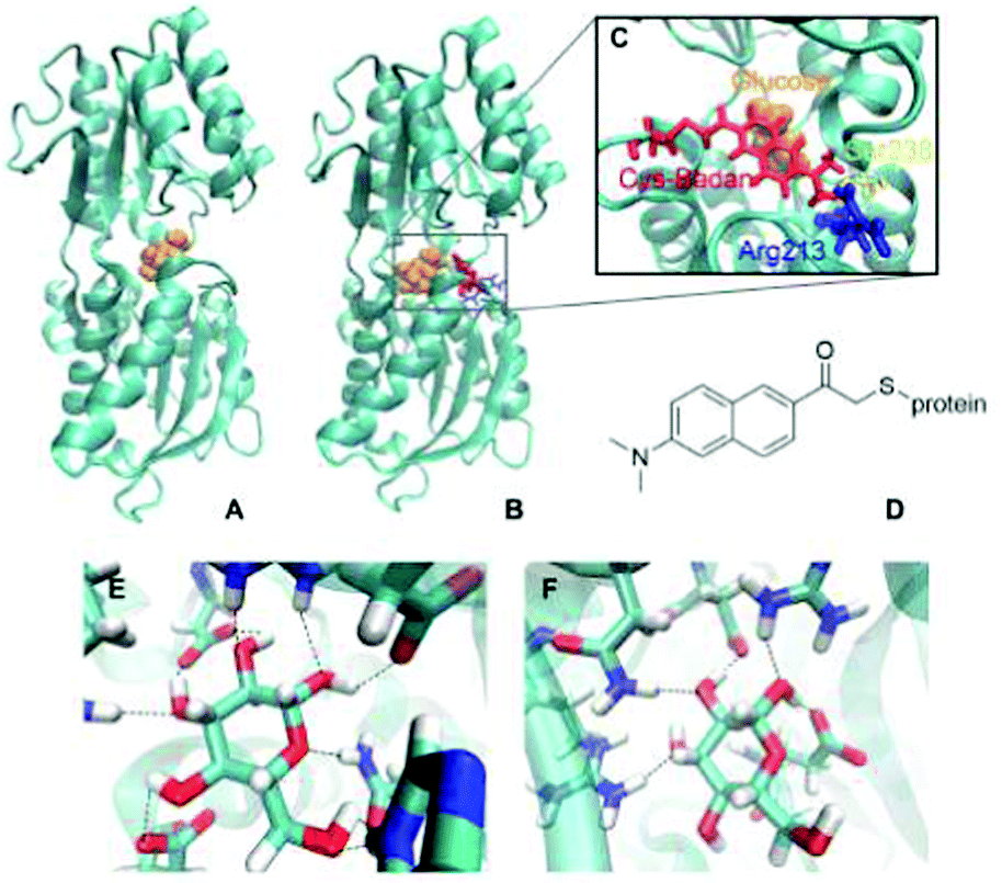Fig. 1 (A) Wild-type closed state GGBP. (B) GGBP triple mutant H152C/A213R/L238S in its closed state. (C) The binding pocket of the triple mutant. Glucose – orange; Cys-Badan – red; Arg213 – blue; Ser238 – yellow. (D) Chemical structure of Badan linked to the protein via a cysteine side chain. The H-bonds between glucose and (E) the wild-type protein or (F) the GGBP triple mutant are shown by dashed lines. Some of H-bonds are missing due to the mutation.

The chemical structure of Badan (as linked to the side chain of Cys152 in the triple mutant) is shown in Fig. 1D. It contains an electron-donating dimethylamino group and an electron-withdrawing carbonyl group with maximal distance from each other on the two sides of the naphthalene core, making it a push–pull charge-transfer system.¹³ The first dye of this kind, Prodan, was synthesized by Weber and Farris.¹⁴ In contrast to Prodan, Badan in its original form contains a thiol-reactive bromine and thus can be linked specifically to a cysteine side chain. Badan is a frequently used environmentally sensitive dye that changes its fluorescence properties depending on the polarity of its surroundings. In the triple mutant, the fluorescence intensity and excited states lifetime change upon glucose binding. So far, it has been assumed that the environment of Badan is more hydrophobic when the protein is in the closed conformation while binding the glucose.⁹ However, there is no crystal structure of the triple mutant, therefore, the overall structure, the details of the binding pocket and the actual Badan conformations, depending on the details of the binding site, are unknown. Consequently, the reason for the change of fluorescence upon glucose binding is unclear, too.

With the development of computers and nanoscale modelling, molecular dynamics (MD) simulations on biological macromolecules have become affordable, and it is now possible to study the GGBP mechanism in atomistic detail. Recently, Unione et al. investigated the wild-type GGBP employing steered MD simulations (SMD).¹⁵ The free energy surface was estimated by the combination of two SMD trajectories, which included the protein opening with glucose and closing without glucose. Due to short simulation times, no continuous free energy map was computed, rather, the information resulting from individual MD simulations of open and closed state was plotted in a single energy scheme. Therefore, the GGBP opening-closing motion and the free energy surface was inferred from two individual hundred-nanosecond free MD trajectories, also including information from NMR measurements. Furthermore, only one collective variable (CV) was used in the SMD, which tends to be a too limited representation of the system's degrees of freedom, since the binding site of the GGBP is buried and the configurational entropy contribution may be large.¹⁶ Panjaitan et al. also reported several short free MD trajectories to study the wild-type GGBP.¹⁷ They found that the protein was unlikely to close after introducing the glucose ligand into the binding pocket, which is in contrast to the experimental findings. The authors argued that this may be due to the insufficient length of the simulations. In fact, it is a challenge for a hundred-nanoseconds free MD simulation to explore a large conformational change when facing a barrier significantly exceeding 3 kcal mol⁻¹, especially for large biomacromolecules like the GGBP.

According to the experimental dissociation constants (0.2 mM for the wild-type and 11 mM for the triple mutant), a free energy difference between apo-open (without glucose in the binding pocket) and holo-closed states (with the glucose in the binding pocket) of 9.2 kcal mol⁻¹ is expected for the wild-type protein.¹ A value of 2.7 kcal mol⁻¹ was reported for the triple mutant with Badan.⁹ However, our initial simulations did not show a stable bound state over 1 μs, as detailed below, a similar finding as reported in the two previous simulation studies. In fact, a stable bound state for several hundreds of nanoseconds has never been reported so far. In one of our simulations the closed state opens within 100 ns of simulation time, which leads to an immediate glucose unbinding in contradiction to the experimental k_D. This may point at a shortcoming in the simulation protocol.

In fact, the H-bonds stabilising the bound state seem to be too weak in the simulations, in order to keep the binding pocket closed on the expected temporal scales. The GLYCAM parameters used here and in the previous computational studies are derived for use with the TIP3P water model.^18,19 However, the glucose molecule bound in the GGBP pocket is highly polarised by several strong H-bonds as shown in Fig. 1B. Therefore, the GLYCAM charge model may not describe glucose in such polarising environments appropriately.

The importance of polarisation effects on force field parameters, in particular on the force field charges was pointed out in several studies of protein–ligand binding,^20–23 peptide folding,^24,25 and protein–chromophore complexes.^26,27 Standard force field parameters, in particular the force field charges, can lead to structural instabilities or even a wrong description of the respective systems. This was previously tackled by explicitly considering the polarisation induced by the specific environment, using one of several approaches. The most accurate but also computationally demanding way is the use of a polarisable force field, where the atomic charges are determined in an iterative procedure. Computationally less demanding is the use of polarised protein-specific charges (PPC), which are computed in order to represent the specific polarised electrostatic state of the protein. The polarised charges are usually determined for one representative structure, but also charge update schemes have been proposed.^24,28 Typically, PPC are determined using a molecular fractionation with conjugate caps (MFCC), followed by the calculation of the electron density of the fragments using DFT with a subsequent restrained electrostatic potential fit (RESP).²⁹ If PPC for a whole protein are to be determined, an iterative procedure is chosen where the charges of the various fragments are recalculated until convergence is reached, while the charges of the remainder of the protein are represented by point charges. It is also possible to fit only the charge variation (delta-RESP) instead of using the conventional RESP approach for charge fitting.^30,31

The importance of considering polarisation effects was demonstrated for several examples: Mei et al. reported that the melting temperature of a small Trp-cage protein obtained from the simulation was only in agreement with the experiment when PPC were applied.²⁵ Tong et al. reported that in contrast to Amber charges, PPC kept the studied light-harvesting complex stable during the simulation and provided also a reliable description of the environment in QM/MM calculations on the chromophores.²⁷ For protein–ligand binding, Duan et al. showed that the binding energies of complexes of the cycline-dependent kinase (CDK2) with five different ligands agree significantly better with experiment using PPC charges than with the unpolarised Amber charges.²²

In this work, we follow these earlier studies and develop force field parameters that account for the highly polarised protein environment. In a second step, these charges are applied in free MD simulations to investigate bound and unbound structures of wild-type GGBP, as well as the GGBP-Badan triple mutant. These parameters lead to a stable glucose binding pocket with a preserved number of H-bonds compared to the initial structure. Further, the overall structure of the protein remains stable, in contrast to the standard GLYCAM charge model. Metadynamics simulations applying these charge models are then performed to achieve a more detailed insight into the mechanism and energetics of the opening and closing mechanism.

2 Methods

2.1 Initial structural model and the force field

The initial structure of the wild-type GGBP and the GGBP-Badan triple mutant (hereafter referred to as the ‘triple mutant’) were taken from the closed GGBP crystal structure, PDB ID 2FVY.³² For the triple mutant, the residues His152, Ala213 and Leu238 were replaced with cysteine, arginine and serine residues, respectively, and the side chain of Cys152 was functionalized with the Badan fluorophore, see Fig. 1D. These changes were performed with the xLeap tool from the AmberTools package.³³ The following force fields were employed: Amber14SB for the protein,³⁴ general Amber force field (GAFF) for the newly parametrized Badan moiety,^35,36 Joung–Cheatham parameters for the ions,³⁷ and GLYCAM 06j for the glucose.¹⁹ Additionally, new atomic charges for the glucose were derived as detailed in the following, and bonded parameters were taken from GAFF.

2.2 Polarised force field for the glucose molecule

Initial simulations employing the standard GLYCAM 06j atomic charges for glucose showed no stable binding to the proteins, as detailed in ESI-S1 (ESI†). Similar findings have been repeatedly reported in the literature for a diverse set of systems: there is a large body of evidence that standard force fields with a fixed point charge model fail to describe H-bond strengths with sufficient accuracy for a variety of systems.^20–27 This seems to apply also for the case of GGBP: in pilot simulations, we were unable to find a stable glucose bound state. The H-bonded network broke and set the glucose free, in contrast to the stable bound state found in experiment. This indicates that the GLYCAM 06j charge model may be insufficient to describe the strong H-bonded network of the GGBP binding pocket, as described above. Here, the glucose molecule is located in the highly polar protein binding pocket, restricted to one stable conformation, which seems to be very different from the more weakly bound floppy structure embedded in water solvent described by TIP3P water, for which GLYCAM 06j is parametrised.

For GGBP–glucose binding, we consider the major source of error to be the glucose charges. Therefore, we decided to only update those and leave the protein charges unchanged. This makes the procedure particularly simple as it is non-iterative and glucose charges are determined only for a single conformation, the bound state of the protein. Update schemes developed to follow conformational changes of proteins²⁴ seem to be less practical for the GGBP–glucose binding case. The focus is on enhanced sampling simulations of the binding–unbinding reaction, during which the glucose is moving back and forth between the protein and water environments which would require a frequent charge update making the calculations computational expensive. Using the charges for the protein-bound state will lead to less accurate charges for the water-solvent case, an error which we will estimate using alchemical free energy calculations as described below.

Two different new sets of atomic charges were created for the glucose polarised in the binding pocket, one for the wild-type protein complex and one for the triple mutant. The procedure started by docking the glucose molecule into the binding pocket of the closed protein, either the wild-type GGBP or the triple mutant, which was subsequently immersed in a TIP3P water box. Standard force field parameters were assigned to the entire system, including the standard GLYCAM 06j atomic charges for the glucose. Then, energy minimisation was performed with steepest descents.

The resulting glucose conformation was taken as input for HF/6-311G* ESP calculations, where atomic charges were subsequently determined with RESP. To account for the polarising environmental effects, we included the force field point charges of the apo-protein up to a certain cutoff radius. This was performed twice, for the wild-type protein and the triple mutant, leading to two different sets of binding pocket polarised charges (BPC) for each specific molecular complex. To estimate possible errors due to a hard cut-off, the results from two different approaches were compared: First, atomic charges from atoms within different cutoff distances from 5 Å to 8 Å from the glucose were included. In the other approach, a residue-based cutoff was applied, including all residues for which at least one atom is found within certain distances. No obvious difference was observed in pilot free MD simulations of 50 ns, see ESI-S2 (ESI†), and the charges determined for an atom-based cutoff at 5 Å were used in the following.

In addition, we also computed a third set of charges for the glucose molecule in aqueous solution. Glucose was optimised at the B3LYP/6-31G* level in the presence of implicit water represented by the polarisable continuum model (PCM).³⁸ Then, the electrostatic potential was computed at the HF/6-31G*/PCM level, and a set of atomic charges was obtained with RESP; this charge model will be referred to as water polarised charges (WPC).

We further computed a gas-phase charge model (GPC) using the same methodology, and in addition, a charge model based on DFTB Mulliken charges. For the latter, two QM/MM simulations were performed using GROMACS:^39–42 one with the glucose in water and one with the glucose in the binding pocket. The sugar was treated with the semi-empirical DFTB/3OB method^43,44 using DFTB+,^45,46 and the environment was described with a force field. These calculations were intended to investigate charge fluctuations along trajectories, and are detailed in ESI-S3 (ESI†). However, DFTB Mulliken charges turned out to be largely underpolarised, therefore, they are not further considered in this work.

2.3 Free MD simulations

We performed three free, unrestrained MD simulations of the wild-type GGBP with a bound glucose molecule: one with the GLYCAM force field for the glucose, one with the BPC, and one more with the WPC charge model. In addition, free MD simulations under the same conditions were carried out on the GGBP-Badan triple mutant with the BPC as well as the WPC glucose, on the triple mutant without glucose and on the wild-type GGBP without glucose.

In all of these simulations, the protein–glucose complex was embedded in a dodecahedral TIP3P water box keeping a distance of the solute from the edges of the box of at least 20 Å. There is a calcium ion bound to GGBP, and electroneutrality was achieved by replacing six water molecules by sodium ions. No extra salt was added. Periodic boundary conditions were applied and long-range electrostatics was described by the particle–mesh Ewald method.⁴⁷ Each simulation was carried out with cut-offs of 1.4 nm for both vdW and real-space PME interactions.

The equilibration procedure started with a steepest descents minimisation to reduce all forces below 1000 kJ mol⁻¹ nm⁻¹, followed by a conjugate gradient minimisation until all forces dropped below 500 kJ mol⁻¹ nm⁻¹. Then, the system was heated to 298 K during an NVT MD simulation of 1 ns with a time step of 2 fs using the Bussi thermostat.⁴⁸ Here, the lengths of all bonds were kept constrained to their respective equilibrium values by means of the LINCS algorithm. Subsequently, an NPT simulation of 1 ns with a time step of 2 fs was performed at a temperature of 298 K and a pressure of 1 bar maintained by the Nosé–Hoover thermostat^{49, 50} and the Parrinello–Rahman barostat,^{51, 52} respectively. Position restraints with a force constant of 1000 kJ mol⁻¹ nm⁻² were imposed on all of the protein atoms during the equilibration procedure above. Finally, the system was equilibrated for further 10 ns keeping only bonds involving hydrogen atoms constrained with LINCS. Identical settings were used to carry out the actual production simulations of 1 μs.

2.4 Well-tempered metadynamics simulations

To further investigate the binding of glucose and the opening of the binding pocket, well-tempered metadynamics simulations⁵³ were performed for both the wild-type GGBP and the triple mutant. These were started from each respective closed structure and involved the atomic charges on the glucose molecule that were polarised for each respective binding situation, as described above. Two collective variables (CV) were employed based on previous work by others:^{15, 54} The opening–closing motion is described with the angle θ between centres of mass of the N-terminal domain (residues 3–108 and 258–291), the hinge region (residues 109–111, 255–258 and 292–296) and the C-terminal domain (residues 112–254 and 297–306). The twisting motion is described with the torsion angle ϕ defined by the centres of mass of the N-terminal domain, the N-terminal domain base (residues 109, 258 and 292), the C-terminal domain base (residues 111, 255 and 296) and the C-terminal domain. These CVs are illustrated in Fig. 2 and were also used to analyse free MD trajectories in the following discussion. Besides, a set of restraints was imposed on the protein as well as the glucose molecule to maintain the stability of the protein structure and to concentrate the sampling process on the binding/unbinding of glucose and opening/closing of the binding pocket; these are described in detail in ESI-S4 (ESI†). With a time step of 1 fs and a bias factor of 10, the metadynamics simulations were extended to 2.6 μs for both wild-type and the triple mutant, respectively.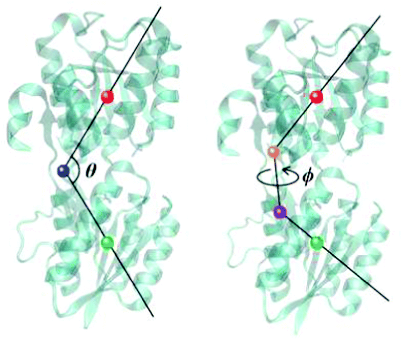

Fig. 2 The collective variables used to describe GGBP. Left: θ, representing the closing–opening motion; Right: ϕ, representing the protein twisting motion. The centres of mass of respective parts of the protein that define the angle/torsion are shown as solid balls. N-terminal domain – green, C-terminal domain – red, hinge region – blue, N-terminal domain base – purple and C-terminal domain base – orange.

2.5 Alchemical free energy calculations and funnel metadynamics simulations

The binding–unbinding simulations were performed with a fixed-charge model. This BPC charge set, however, is optimised for the glucose molecule in the binding pocket, and may yield overestimated solvation free energy of glucose in water. To take into account the change of charge distribution on the glucose molecule upon unbinding from the protein, a series of free energy simulations was carried out for both the wild-type GGBP and the triple mutant, as follows. The resulting free energy shall give an estimate of a possible error in the free energy profiles obtained from the simulations described above.

First, alchemical simulations were performed to obtain the glucose binding energy difference when passing from the BPC glucose charges to GLYCAM charges, with the protein binding pocket remaining in the open state. The respective wild-type and triple-mutant BPC charge models were used here. Second, funnel metadynamics simulations⁵⁵ were carried out using the GLYCAM glucose charges to obtain the free energy of unbinding. In all of these simulations, the protein structure was constrained at the corresponding open state local minima obtained by well-tempered metadynamics simulations for the respective protein (wild-type or triple mutant GGBP). All sets of alchemical simulations contain 21 λ windows with a spacing of 0.05, each consisting of an MD simulation of 4 ns. All funnel metadynamics simulations were extended to 750 ns to achieve convergence. More details about the settings of funnel metadynamics simulations can be found in ESI-S4 (ESI†).

2.6 Software

Free MD simulations and alchemical calculations were carried out with Gromacs 2018.3. Well-tempered metadynamics simulations and funnel metadynamics were performed with PLUMED 2.5^56,57 linked to Gromacs 2018.3. Molecular structures were constructed and visualised with VMD 1.9.2.⁵⁸ Quantum chemical calculations were performed with Gaussian09,⁵⁹ and RESP was run with Antechamber.^33,60

3 Results and discussion

3.1 Polarisation of the glucose molecule

The wild-type GGBP has a k_D of 0.2 mM,¹ corresponding to a binding free energy of ca. 9 kcal mol⁻¹, which means that at least hundreds of microseconds would be needed to see a change from the holo closed state to the apo open state. However, when employing the GLYCAM parameters for glucose, the wild-type GGBP changed from its closed state to an open state within hundred nanoseconds, which is orders of magnitude faster than expected, see ESI-S1 (ESI†). This finding agrees with previous studies,^15,17 where no wild-type GGBP closed state simulation for several hundreds of nanoseconds is reported. It further indicates that the ligand in the binding pocket may not be sufficiently stabilised during the MD simulations, most probably due to too weak H-bonds as a result of the applied GLYCAM 06j charge model.

We applied a polarised charge scheme for glucose. Two sets of polarised charges were derived for the wild-type and triple mutant (BPC) binding pockets, one for bulk water (WPC) and one for the gas-phase (GPC). The charge models are given in ESI-S3 (ESI†). We assigned these polarised charges to glucose and performed a set of 50 ns MD simulations for the glucose in the two binding sites, respectively.

As shown in Fig. 3, the H-bonded network of the wild type stays intact when using the BPC and WPC charges. We find an average of nine H-bonds between the glucose and the binding pocket, which is the number of H-bonds also found in the crystal structure as indicated in Fig. 1E. By contrast, when using the GLYCAM charges, there are much fewer H-bonds, which frequently break so that the binding pocket opens. As discussed below, the free energies of opening/closing of the binding pocket agree very well with the experimental values, supporting the use of such polarised charges.

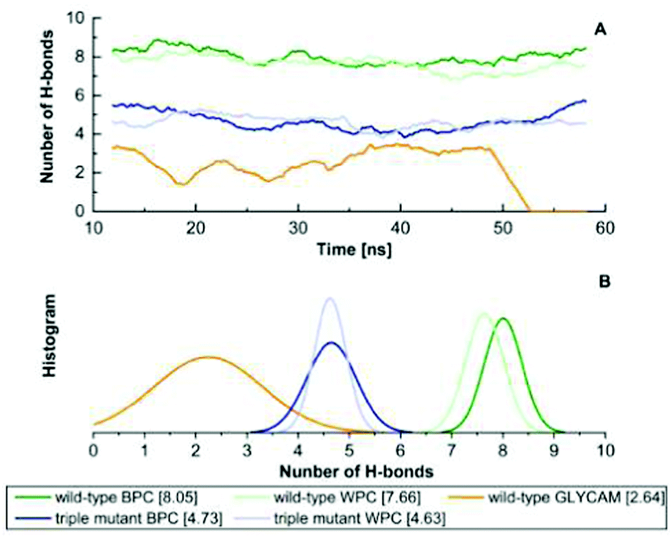Fig. 3 (A) The number of H-bonds formed between the binding pocket and the glucose polarised in different environments. (B) The histogram of the number of H-bonds observed in simulations run with the different glucose charge models. The average number of H-bonds of each corresponding glucose is given in square brackets. Trajectories are taken from corresponding free MD simulations from 10 ns to 60 ns. For the wild-type protein with GLYCAM charge glucose, the ligand escaped from the binding pocket at ca. 50 ns.

For the mutant, a smaller number of H-bonds is found as indicated in Fig. 1F. The change in the experimental k_D indicates such a behaviour, and again, the agreement with experimental estimates of the unbinding free energies supports the usage of these charges.

The use of fixed polarised charges has some drawbacks, which can only be avoided using a fully polarisable electrostatic model in principle. The dynamical transitions, i.e. the opening and closing of the binding pocket and unbinding and binding of the glucose seem to ask for a change of the charge model during the process, since the polarisation of glucose in solution differs from that in the binding pocket obviously. One way to deal with this could be the usage of an average model, however, we decided to use both BPC and GLYCAM models in the simulations and critically discuss the results. Using the BPC model, glucose could be overstabilised in the solution phase due to the larger dipole moment, while using the GLYCAM model glucose is most probably understabilised in the binding pocket. Since we are interested in the kinetic barrier for unbinding, we use the BPC models for the simulations and discuss corrections to this polarised model below.

3.2 Molecular dynamics simulations of the wild-type

The collective variables, θ and ϕ (see Fig. 2), adopted for metadynamics simulations in this study, were also used to analyse free MD trajectories, as described in the methods section. The corresponding values for the crystal closed (PDB-ID: 2FVY) and open (PDB-ID: 2FW0) wild-type GGBP are shown in Table 2. As discussed above, we performed MD simulations with both charge models, the WPC and BPC charges.

Table 2 Collective variable values for the crystal wild-type GGBP

Collective variable	Closed GGBP	Open GGBP
θ	121.6°	143.1°
ϕ	64.9°	89.6°

---

Fig. 4 shows the results of three extended MD simulations of over 1 m s each: In the first two simulations, we used the WPC and BPC glucose charges and started the simulations from a crystal closed state GGBP structure. The protein remained in a stable closed state in both simulations with the glucose molecule inside the binding pocket. Both free MD simulations show a root-mean-squared deviation (RMSD) with respect to the crystal closed wild-type below 0.2 nm, and keep the distance between the glucose and the centre of the binding pocket within 0.3 nm during the simulation of 1 μs. It is interesting to see that both WPC and BPC glucose charges lead to a stable bound state for 1 μs, which is in agreement with the experimental k_D value and is in contrast to the results using the original GLYCAM parameters.

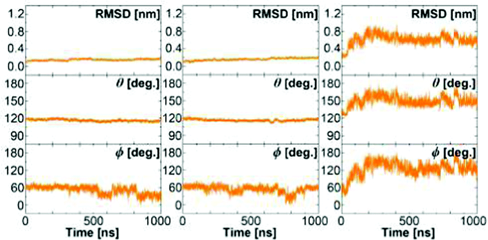Fig. 4 The structure of the wild-type protein in the free MD simulations of the wild-type GGBP. Left: Simulation started at crystal closed state with BPC glucose; Middle: Simulation started at crystal closed state with WPC glucose; Right: Simulation started at crystal open state without glucose. RMSD from the closed GGBP crystal structure (2FVY) is considered. The angle θ describing the opening-closing motion of GGBP and the dihedral ϕ describing the twisting of the domains (details in text) are plotted versus simulation time.

As already mentioned, the glucose molecule is strongly H-bonded in the highly polar binding pocket, therefore, it is expected that the molecule is polarised to a large degree, and parameters derived for a less polar and less strongly H-bonded environment may not optimally describe this situation. The results therefore indicate that the reparametrisation seems to be the right way to go. That alone, however, is not a justification for this approach: more evidence comes from the calculation of the free energies of binding/unbinding, as described below. The fact that the newly derived parameters are able to describe these energies for both, wild-type and mutant with largely different energetics, is highly encouraging.

In the third simulation, which was started from the crystal open state GGBP structure without glucose, the protein immediately closed and then changed its conformation back to the open state after 50 ns. At this point, we like to note that the open structure seen in the X-ray experiment³² had been crystallised at high salt concentration – different from our simulations that are closer to low-salt, physiological conditions. This may be a reason why the stable open state structure from simulations deviates from the experimentally observed wild-type open structure. The RMSD compared to the wild-type crystal closed structure correspondingly dropped from 0.4 nm to 0.2 nm and then increased up to 0.6 nm, indicating that the wild-type protein is unlikely to remain in a closed state without the glucose.

Besides, as shown in Table 3, the structures along these three trajectories exhibit a highly similar average θ value of 116° in the closed state and 152° in the open state similar to the θ values reported previously in ref. 15 and 54. In the closed state, the ϕ value fluctuates around the crystal structure value of 65°. The regions of lower ϕ values of about 20–30° indicate a twisted closed state, which we will discuss in more detail below. In the open state, the average ϕ value is ca. 40° larger than the crystal open structure value of 90°. This increased flexibility with respect to the crystal structure may be expected due to the removal of the crystal packing constraints in the simulations of GGBP in aqueous solution.

Table 3 Average values of θ and ϕ and their deviations compared to the crystal wild-type GGBP

Collective variables	θ		ϕ
	Average	Deviation	Average	Deviation
Wild-type closed state	116.3°	5.3°	51.3°	13.6°
Wild-type open state	151.7	+8.6	132.7	+43.1
Triple mutant ‘cc’ state	127.5	+5.9	76.8	+11.9
Triple mutant ‘cc*’ state	124.1°	+2.5°	69.7°	+4.8°
Triple mutant ‘tc’ state	116.7°	4.9°	76.3°	+11.4°
Triple mutant ‘tc*’ state	127.1°	+5.5°	85.9°	+21.0°
Triple mutant ‘tc**’ state	128.1°	+6.5°	128.6°	+63.7°
Triple mutant ‘op’ state	145.1°	+2.0°	126.5°	+36.9°
Triple mutant ‘op*’ state	154.0°	+10.9°	137.0°	+47.4°

---

3.3 Molecular dynamics simulations of the triple mutant

Just like for the wild type, we performed a set of three MD simulations of 1 μs each for the GGBP triple mutant. The results from the analysis of structures along the trajectories are shown in Fig. 5. Recall that since no crystal structure is available for the triple mutant, the crystal structures of the wild-type protein, 2FVY and 2FW0 were considered as initial structures after manual mutation of the three residues. In the following, the label ‘crystal structure’ refers to the mutated 2FVY initial structure. Due to the mutations, the glucose is much less tightly bound, as the experimental k_D value indicates, and we indeed see a more dynamical behaviour already on this microsecond scale.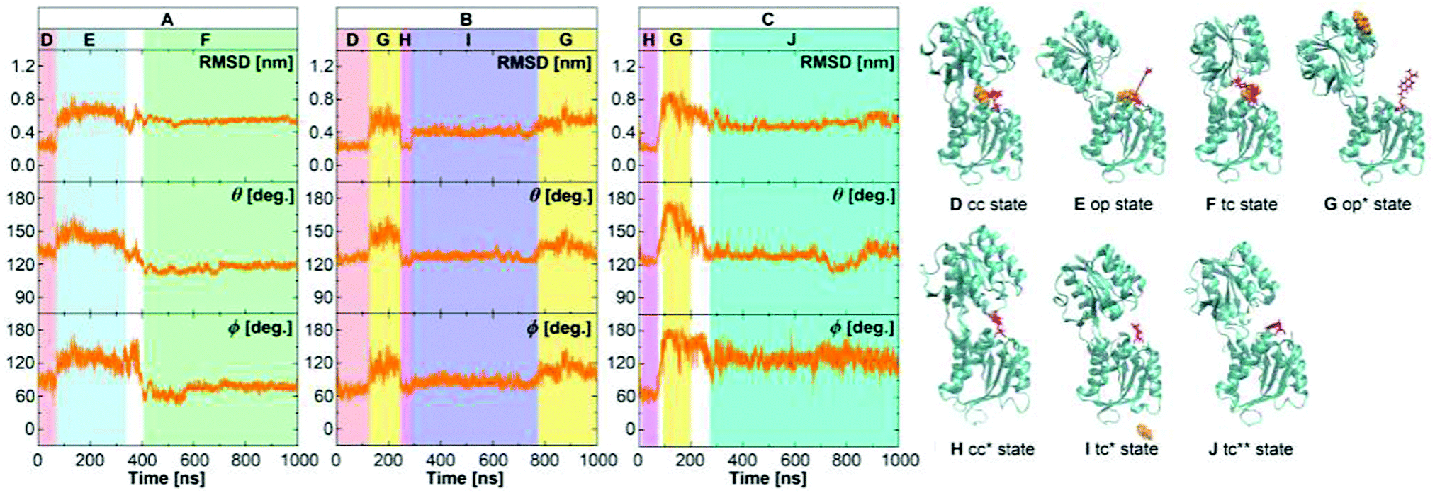

Fig. 5 The structure of the GGBP triple mutant protein in the free MD simulations of the GGBP triple mutant. The RMSD was calculated compared to the backbone of closed wild-type GGBP crystal structure (2FVY). The glucose is coloured with orange and the Cys-Badan residue with red. (A) Simulation with the BPC glucose started with a holo crystal closed state. (B) Simulation with the WPC glucose started with a holo crystal closed state. (C) Simulation without the glucose started with a apo crystal open state. The red region represents holo crystal closed (cc) state; The pink region is apo crystal open (cc*) state; The blue region represents holo open (op) state; The yellow region represents apo open (op*) state; The green region represents holo twisted closed (tc) state; The purple region represents apo twisted closed (tc*) state; The cyan region represents apo super-twisted closed (tc**) state. Schematic representation structures D, E and F were taken from trajectory A, G and I from trajectory B, H and J from trajectory C, respectively.

As seen in Fig. 5A for the BPC model, the protein changes from a crystal closed state (cc) to an open state (op, red to blue) after 70 ns. After ca. 200 ns, the protein returns to a metastable twisted closed state (tc, blue to green). Although the protein was open for a significant amount of time, the glucose did not leave the binding pocket entirely. Rather, it interacted with the residues of the C-terminal domain, so that the bound state is recovered after closing. This state shows slightly larger values of the dihedral angle, and is therefore called a twisted closed state labelled ‘tc’. The deviation from the wild-type GGBP can be expected due to less stable H-bonds, as described above. The bound structure is schematically shown in Fig. 6D, and comparison with the wild type in Fig. 6C shows the dramatically reduced H-bonding of this variant.

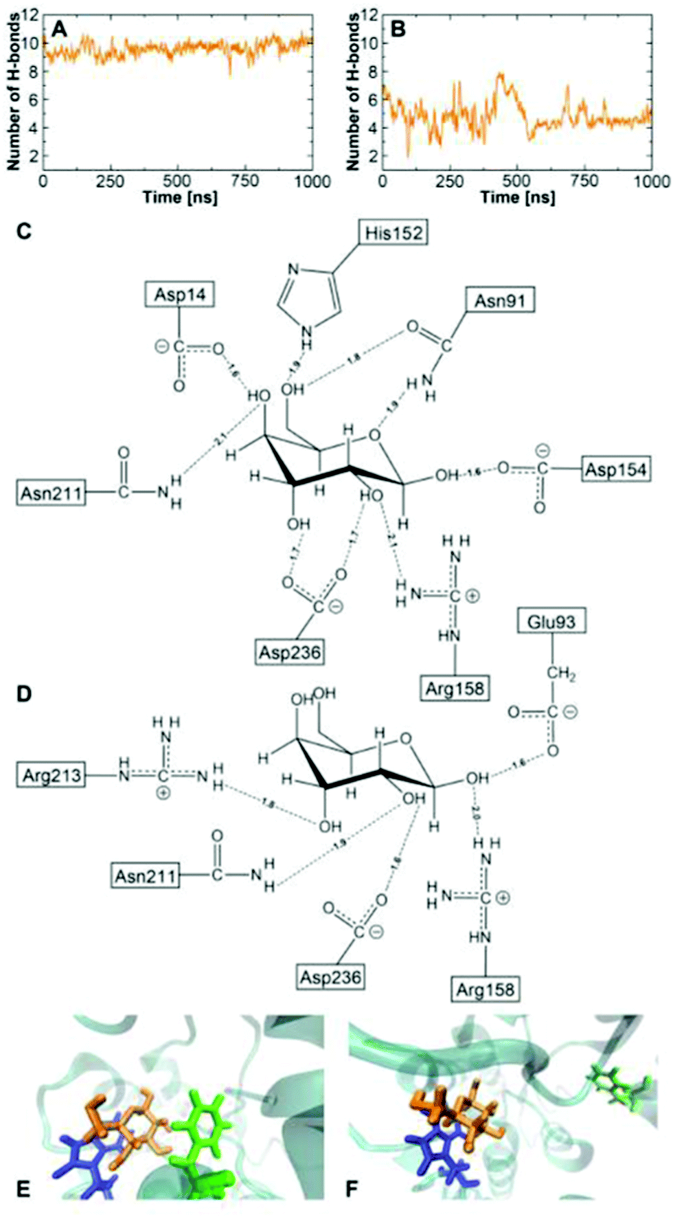Fig. 6 The average number of H-bonds between glucose and the GGBP side chains along the free MD trajectories of wild-type GGBP with BPC glucose (A) and triple mutant with BPC glucose (B). (C) schematic representation of the H-bond pattern in wild-type at 500 ns, the protein is at a crystal closed state and there are 9 strong H-bonds; (D) schematic representation of the H-bond pattern in the triple mutant at 750 ns, the protein is at ‘tc’ state and there are 5 strong H-bonds; (E) the carbohydrate–π interaction between glucose and the wild-type binding pocket; (F) the carbohydrate–π interaction between glucose and the triple mutant binding pocket. The glucose–Phe16 interaction is missing due to the mutation. Glucose – orange; Phe16 – green; Trp183 – blue.

In the simulation with WPC glucose (Fig. 5B), an unbinding process occurs as well as large conformational changes of the protein: first, an opening and closing process are observed (from red to pink), the glucose leaves the binding pocket at ca. 200 ns when the protein is in the open state during this period. Afterwards, the protein deformed from the crystal closed state (cc*) into a twisted closed state (tc*, from pink to purple), which is stable for almost 500 ns without containing glucose in the binding pocket. Finally, the protein opens again (from purple to yellow). Note that the labels with asterisk denote apo states, while the labels without asterisk stand for holo states, as found during the different simulations.

To investigate the dynamics without glucose (Fig. 5C), a simulation was started from the crystal open structure. The protein immediately changed to the crystal closed state (cc*). After 70 ns, the protein returned to the open state (from pink to yellow) before finally reaching a super-twisted closed state (cc**, from yellow to cyan). Note that – just like in the case of the wild-type – our simulation system has no extra salt, while the X-ray structure had been resolved in experiments performed at high salt conditions.^7,9 This is a possible reason for the open state structure in simulations deviating from the crystal open state. Furthermore, the mutations in the protein may also have affected the structure and stability of the open state.

Events occurring along single trajectories, however, may not be conclusive to evaluate the different parameter sets used. We therefore use the insight from these simulations merely to determine intermediate structural motifs, which we will use to interpret the free-energy simulations as discussed below. Having now stable structures for sufficiently long temporal scales allows us to characterise these structures in solution and compare to the crystal structure.

For both simulations with glucose, average θ values at crystal closed (red and pink region, ca. 125°) and open (blue and yellow region, ca. 150°) state agree well with the crystal wild-type GGBP (θ = 122° and 143°), as shown in Table 3. The θ value at ‘tc’ state (green region, ca. 117°) is, like the wild-type closed state, ca. 5° smaller than the crystal closed state, which indicates that the twisted state is slightly more closed.

Larger deviations from the wild-type crystal structure are found for ϕ, see Table 3. The crystal closed states have average ϕ values between 51–77°. The open states have ϕ values beyond 90° extending to 180° (Fig. 5C, yellow region); the twisted closed states have an average ϕ value of 76° and 86°; the super-twisted closed state has an average ϕ value of 129°. In summary, compared to the closed crystal structure, the wild-type as well as the triple mutant in solution show metastable states which are similarly closed but twisted, while both twist directions are possible. Compared to the wild-type open crystal structure, the structures of the wild-type and triple mutant proteins in solution are more open and significantly more twisted.

Fig. 6 illustrates the average number of H-bonds between the glucose and the side chains of the proteins. Using the BPC parameters, nearly nine H-bonded interactions are found for the wild-type protein in the crystal closed state, which is close to the experimental estimate.^1,61 Only half of the H-bonds remain between the BPC glucose and the GGBP triple mutant in the twisted closed state. In the ‘tc’ state, Arg213 forms an H-bond to the glucose molecule as shown in Fig. 6. Additional H-bonds are formed with Arg158, Asp236, Asn211 and Glu93. The latter is not interacting with glucose in the wild-type. Compared to the wild-type, the triple mutant's twisted closed state misses H-bonds to Asp14, Asn91, Asp154 and the mutated residue 152. As a result, the glucose hydroxyl groups are not interacting with protein residues, and they form H-bonds with solvent water molecules instead. In the wild-type, the glucose is additionally stabilised by two aromatic residues Phe16 and Trp183. In the triple mutant, Phe16 moves away from the glucose molecule and the stabilisation due to the aromatic sandwich structure is missing, as seen in Fig. 6E and F.

3.4 Free energy surfaces

To explore a full free energy surface (FES) of the closing–opening motion of the protein, metadynamics simulations of wild-type and triple mutant were performed beyond 2.5 m s until convergence. We chose the BPC charge model because a proper description of the bound state has to be assured for the unbinding barrier to be overcome. This means, however, that the free energy of solvation in the water bulk phase may be described less accurately.

The FES of wild-type GGBP is shown in Fig. 7A, with well defined closed and open states denoted by a and b. The CV values at the global minimum a, θ ≈ 120° and ϕ ≈ 30°, agree well with the results from the free MD simulations discussed above. The CV values of state b, θ ≈ 160° and ϕ ≈ 170°, are much larger than those reported for the crystal structure. As discussed in ref. 15, a possible reason for this deviation is that the ligand-free crystal structure is stabilised in a more closed state due to the crystallisation reagents. There is a free energy difference of ΔG = 9.4 kcal mol⁻¹ between the closed state and open state, and the reaction barrier is 11 kcal mol⁻¹.

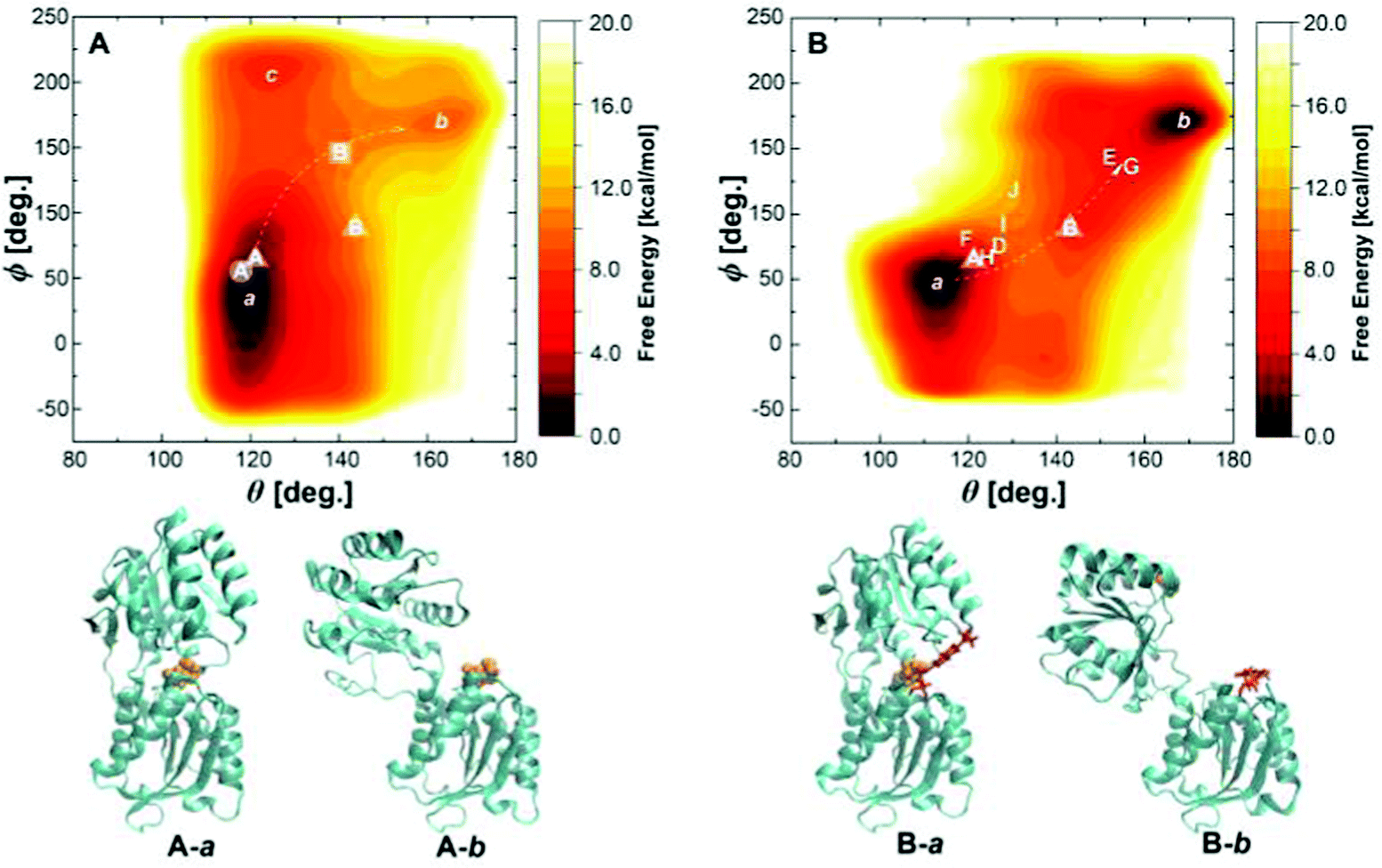Fig. 7 (A) The free energy landscape of the wild-type GGBP with collective variables θ and ϕ. The label with circle represents the holo state, square represents the apo state. State A in circle and B in the square is picked up from free MD trajectories of the wild-type GGBP. (B) The free energy landscape of the GGBP-Badan triple mutant with collective variables θ and ϕ. States D to J are taken from three free MD trajectories of the GGBP triple mutant, and represent the crystal ‘cc’, ‘cc*’, ‘op’, ‘op*’, ‘tc’, ‘tc*’ and ‘tc**’ state as shown in Fig. 5, respectively. States A and B in the triangles indicate wild-type crystal closed and open structures, and the white arrows indicate pathways between the closed and the open states. The corresponding schematic representations of local minima a and b for wild-type and triple mutant are shown as A-a, A-b, B-a and B-b.

We also find a ‘semi-closed’ state c (Fig. 7A), which is twisted compared to the minimum a. Such a state has never been reported before and could be part of an alternative pathway for the closing–opening motion in the wild-type GGBP: the closed protein firstly twists from state a towards state c, which can be seen as an intermediate, and then opens to state b.

The FES of the triple mutant is shown in Fig. 7B with closed state a and open state b. The free energy difference of 0.8 kcal mol⁻¹ is slightly less than the experimental value of ca. 2.7 kcal mol⁻¹,⁹ and the energy barrier of 9 kcal mol⁻¹ is only slightly lower than that of the wild-type. The states D–J discussed for the free MD simulations are distributed along the reaction coordinate connecting the states a and b. Compared to the wild-type crystal closed structure, the state a is a slightly more closed and twisted conformation with θ = 115° and ϕ = 50°.

Comparing wild-type and mutant, a slight difference in conformation and opening mechanism is visible in Fig. 7: The closed state a spans a much wider range of ϕ, i.e., this structure can exist in more twisted conformations, while the global minimum of the mutant is much more localised in the CV space. Further, the opening motion seems to follow slightly different pathways: While a twisting motion along ϕ is followed by an opening of the pocket with increasing θ in the wild-type, the motion in the mutant follows the opposite order.

There are two potentially small imperfections to note. First, the computed energetics clearly depend on the force field parameters. The glucose molecule is located in an unusually strongly polarising environment, which is an extreme situation to deal with. In such a case, the general purpose parameter set does not depict the true distribution of charge, leading to wrong energetics and potentially to qualitative errors in simulations. Here, we have reparametrised the force field charges, which fixed the qualitative failure of the previous simulations. However, with the BPC charges, a glucose molecule is overpolarised in water, which may result in an overstabilisation in water. Second, the position of the glucose molecule is not accessible from the applied CVs. As seen in Fig. S5 (ESI†), the glucose remained at the binding site in both open and close state. The advantage of this is that the closed state is always the glucose bound state in the simulations, and there is no mixture of closed holo and apo states. Therefore, the barrier and free energy of binding in the closed state are described correctly. This is probably due to the fact that the simulations were started with the closed holo states and the reparametrised force field charges were taken for the glucose, and the glucose remained in the binding site during the process of protein opening and closing. For the open state, however, a small error may arise because the unbinding is not described fully.

To account for the over-polarisation of glucose in water and the failure of glucose to unbind in the open state, we compute the glucose binding free energy difference from BPC to GLYCAM charge sets, and the glucose unbinding energy with the GLYCAM charge set, as shown in Table 4. In this way, the free energies of glucose unbinding accompanied by opening of the protein pocket were corrected, see Fig. 8 for the results.

Table 4 Glucose binding free energy difference and unbinding energy (kcal mol⁻¹)

	ΔΔGbinding	ΔGunbinding
Wild-type	0.5	5.2
Triple mutant	0.2	2.6

---

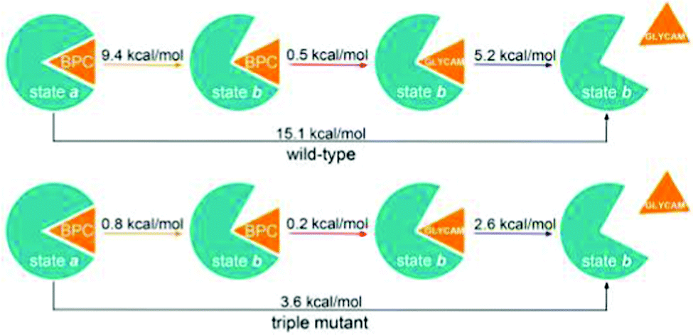Fig. 8 Two series of free energy simulations for protein structural changes from holo closed state to apo open state. Orange arrows – Free energies of holo protein opening from metadynamics. Red arrows – ΔΔG_binding from alchemical simulations. Blue arrows – GLYCAM glucose unbinding energies from funnel metadynamics.

We find a reaction free energy of 15.1 kcal mol⁻¹ for the wild-type and 3.6 kcal mol⁻¹ for the triple mutant. Notably, in the holo open state b, when the glucose leaves the binding pocket, the glucose polarisation by the protein will gradually decrease, and hence the glucose charges will reduce to the GLYCAM charges. This means, with GLYCAM charges in our free energy simulations series, the glucose unbinding energy is slightly underestimated when the glucose starts to leave. Therefore, the reaction free energy between holo closed state and apo open state may be slightly higher than obtained from free energy simulations series.

Note that the experimentally measured k_D may not only describe the process from holo close state to apo open state, rather it may also correspond to the processes from holo close state to apo close state or from holo open state to apo open state, indicated by the large error bars.^{7, 9, 32} For both of the latter situations, the protein conformational changes are missing, leading to a smaller reaction free energy. Therefore, in these cases, the experimental ΔG will be smaller than our binding free energy results. Nevertheless, the agreement with experiment is remarkable, and the computed free energy differences are in line with the qualitative mechanistic picture emerging from the free simulations discussed above: the H-bonded network is destabilised in the mutant, leading to a much weaker binding of glucose, which qualitatively explains the difference in the experimentally reported k_D values.

To resolve the problem altogether, an additional CV describing the glucose position is necessary. However, for that, either a 3D metadynamics simulation needs to be performed (which is computationally highly expensive) or the protein motion needs to be described by only one CV, which carries the risk of missing important regions in the conformational space or of losing the easy interpretability of the result by an abstract CV. Further, a change in glucose polarisation along the reaction coordinate would have to be considered in this case as well, which is a difficult task that would require an explicitly polarisable force field. Still, we believe that our estimates are sufficiently accurate to allow for an insight into the mechanisms, and in particular, to understand the differences between the wild-type and the mutant.

3.5 Conformations of Badan

Besides understanding the change in binding, another key aim of this study is the investigation of Badan conformations and their possible relation to its fluorescence properties. The conformational changes in the protein impact the properties of the excited states of Badan, and it was suggested that the dye resides inside a hydrophobic environment in the protein if and only if a glucose molecule is bound.^{9, 62} Analysis of the MD trajectories allows to investigate the dynamics of the chromophore coupled to the protein conformational changes in more detail.

First, it is necessary to quantify how often Badan is inside or outside of the binding pocket dependent on the protein conformation and presence of glucose. To this end, 2D histograms were obtained with one variable describing the protein conformation and the other variable describing the orientation of Badan. To obtain the 1D coordinate for the protein, a line was constructed connecting the minima a and b found in the metadynamics simulations. The protein conformations are projected onto this line and the values are scaled such that minimum a corresponds to 0 and minimum b corresponds to 1. The orientation of Badan is described by the distance between the nitrogen of its dimethylamino moiety and the nitrogen of Pro239, which is located on the opposite side of the pocket, see ESI-S6 (ESI†). A small distance indicates that Badan is inside the binding pocket, and a large distance means that Badan is somewhere outside.

The 2D histograms showing the relative frequencies of appearance of conformations of protein and Badan, together with representative conformations of Badan are presented in Fig. 9. These data are derived from the MD simulations of the GGBP triple mutant, see also Fig. 5. The binding of glucose correlates with the conformation of Badan clearly: Badan is outside the binding pocket when a glucose molecule is bound, being exposed to a more hydrophilic environment (Fig. 9A and B). For the protein apo state, Badan is mostly located inside the binding pocket when the binding pocket is open (Fig. 9D), in which case it is exposed to a probably more hydrophobic environment (Fig. 9C and D). For the apo closed state (Fig. 9C), the dye is found in- and outside of the binding pocket. These findings are supported by analysis of further MD trajectories and metadynamics simulations, see ESI-S6 (ESI†).

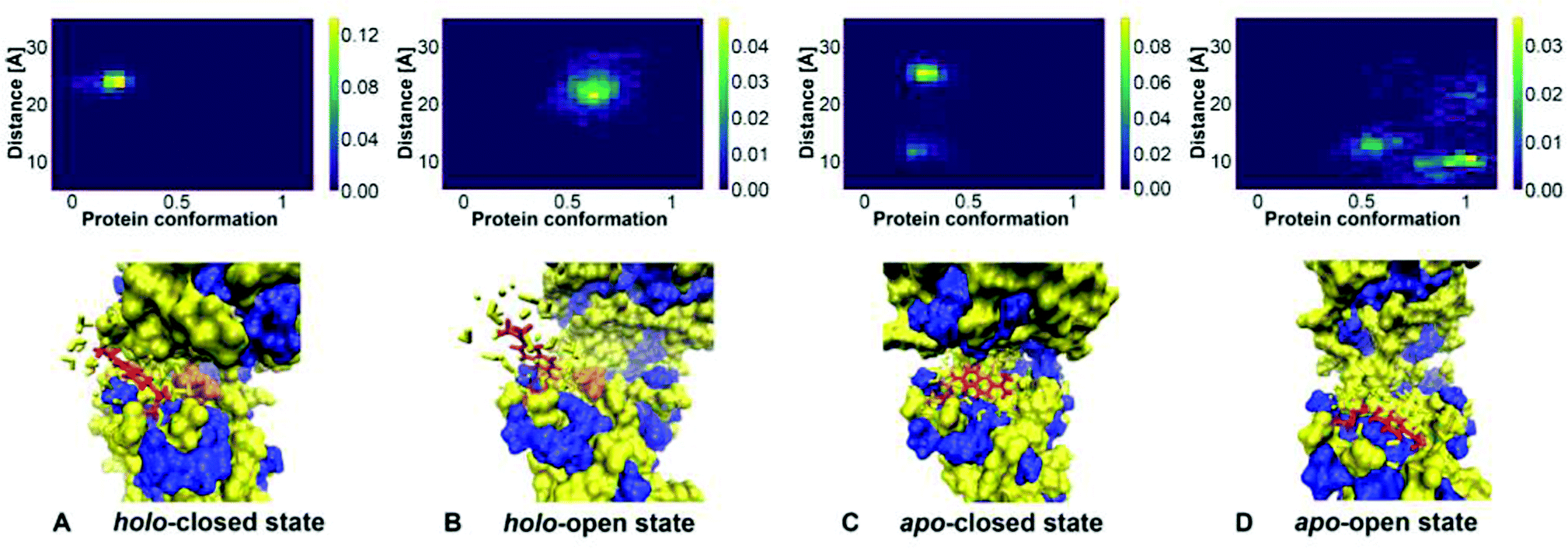Fig. 9 2D histogram of protein conformation and Badan orientation (created with Python 3.9) with corresponding schematic presentations of Badan in hydrophobic/hydrophilic environment. In the normalised histograms, the x-axis represents the line connecting minima a and b from the metadynamics simulations. It is scaled such that 0 corresponds to a and 1 corresponds to b. The y-axis shows the distance between the top of Badan and Pro239. A distance smaller than 15 Å indicates that Badan is inside the binding pocket and a larger distance means that Badan is outside. Protein hydrophobic region – blue; Protein hydrophilic region – yellow; Cys-Badan – red; Glucose – orange. Water molecules within 4 Å away from the Cys-Badan molecule are described as yellow licorice shapes. Structure A to D were take from Fig. 5A–E, A–F, B–G and B–I respectively.

Therefore, the environment of Badan changes upon glucose binding clearly, and is more polarisable, which most probably is responsible for the increase of fluorescence observed experimentally. It was also observed that in the stable conformation of Badan folded inside the binding pocket in absence of glucose, the aromatic core of the dye and Trp183 are in close proximity. This points to another factor for the intensity increase upon glucose binding – the presence of Trp183 in the binding pocket, which is a known quencher of the fluorescence of Badan.^{63, 64}

4 Conclusion

In this work, we aimed at a detailed explanation of the mechanisms of glucose binding in GGBP using classical MD simulations and enhanced sampling techniques. A particular goal is to understand the changes upon mutation, which removes four H-bonds, leading to a drastic increase of k_D.

Up to now, no crystal structure of the triple mutant is available, therefore, our simulations uncover the molecular details of the mutant including Badan conformations for the first time. In particular, the simulations show how the conformation of Badan is coupled to the opening and closing of the binding pocket, and to the presence of glucose. So far, it had been assumed that the environment of Badan is more hydrophobic when the protein is in the closed conformation while binding the glucose.⁹ Our simulations indicate that the opposite is true in fact: in the unbound state, Badan interacts with a Trp side chain, leading to the quenching of fluorescence.

Force field charges turned out to be critical parameters. The standard charge set, developed for bulk solvent, was unable to describe the binding situation in this highly polar and charged environment. Correction of charges by means of reparametrisation lead to a stable binding pocket as well as free energies of pocket opening in a very good agreement with experimental estimates. The series of free energy simulations designed in this work provided additional insight into the processes of interest taking place in such complex protein systems. Hence, such simulations appear capable of supporting the efforts of rational design of new glucose sensors.

The knowledge of the conformational dynamics of Badan allows for further work to investigate the changes of fluorescence of Badan in detail. That will involve excited-state QM/MM simulations using the semi-empirical TD-LC-DFTB method to describe the dynamics of Badan in its excited states.

Conflicts of interest

There are no conflicts to declare.

Acknowledgements

This work was supported by the German Research Foundation (DFG) through project GRK 2039, as well as by the state of Baden-Württemberg through bwHPC and DFG through project INST 40/467-1 FUGG (JUSTUS cluster). Z. P. acknowledges the China Scholarship Council for financial support. The authors thank Annika Enß for her efficient assistance.

Notes and references

1. N. K. Vyas, M. N. Vyas and F. A. Quiocho, Science, 1988, 242, 1290–1295.
2. S. L. Mowbray, R. D. Smith and L. B. Cole, Receptor, 1990, 1, 41–53.
3. J. S. Marvin and H. W. Hellinga, J. Am. Chem. Soc., 1998, 120, 7–11.
4. L. L. E. Salins, R. A. Ware, C. M. Ensor and S. Daunert, Anal. Biochem., 2001, 294, 19–26.
5. R. M. D. Lorimier, J. J. Smith, M. A. Dwyer, L. L. Looger, K. M. Sali, C. D. Paavola, S. S. Rizk, S. Sadigov, D. W. Conrad, L. Loew and H. W. Hellinga, Protein Sci., 2002, 11, 2655–2675.
6. V. Scognamiglio, V. Aurilia, N. Cennamo, P. Ringhieri, L. Iozzino, M. Tartaglia, M. Staiano, G. Ruggiero, P. Orlando, T. Labella, L. Zeni, A. Vitale and S. D'Auria, Sensors, 2007, 7, 2484–2491.
7. F. Khan, L. Gnudi and J. C. Pickup, Biochem. Biophys. Res. Commun., 2008, 365, 102–106.
8. X. Ge, G. Rao and L. Tolosa, Biotechnol. Prog., 2008, 24, 691–697.
9. F. Khan, T. E. Saxl and J. C. Pickup, Anal. Biochem., 2010, 399, 39–43.
10. T. Saxl, F. Khan, M. Ferla, D. Birch and J. Pickup, Analyst, 2011, 136, 968–972.
11. C. Tiangco, D. Fon, N. Sardesai, Y. Kostov, F. Sevilla III, G. Rao and L. Tolosa, Sens. Actuators, B, 2017, 242, 569–576.
12. N. Helassa, J. P. Garnett, M. Farrant, F. Khan, J. C. Pickup, K. M. Hahn, C. J. MacNevin, R. Tarran and D. L. Baines, Biochem. J., 2014, 464, 213–220.
13. R. Adhikary, C. A. Barnes and J. W. Petrich, J. Phys. Chem. B, 2009, 113, 11999–12004.
14. G. Weber and F. J. Farris, Biochemistry, 1979, 18, 3075–3078.
15. L. Unione, G. Ortega, A. Mallagaray, F. Corzana, J. Pérez-Castells, A. Canales, J. Jiménez-Barbero and O. Millet, Chem. Biol., 2016, 11, 2149–2157.
16. S. Raniolo and V. Limongelli, Nat. Protoc., 2020, 15, 2837–2866.
17. B. M. Panjaitan, K. Kubiak-Ossowska, D. Birch and Y. Chen, Mater. Sci. Forum, 2019, 948, 133–139.
18. M. Basma, S. Sundara, D. Çalgan, T. Vernali and R. J. Woods, J. Comput. Chem., 2001, 22, 1125–1137.
19. K. N. Kirschner, A. B. Yongye, S. M. Tschampel, J. González-Outeiriño, C. R. Daniels, B. L. Foley and R. J. Woods, J. Comput. Chem., 2008, 29, 622–655.
20. L. Chang, T. Ishikawa, K. Kuwata and S. Takada, J. Comput. Chem., 2013, 34, 1251–1257.
21. J. Liu, X. He and Z. H. Zhang, J. Chem. Inf. Model., 2013, 53, 1306–1314.
22. L. Duan, G. Feng, X. Wang, L. Wang and Q. Zhang, Phys. Chem. Chem. Phys., 2017, 19, 10140–10152.
23. S. Zhong, K. Huang, Z. Xiao, X. Sheng, Y. Li and L. Duan, J. Phys. Chem. B, 2019, 123, 8704–8716.
24. C. Wei, D. Tung, Y. M. Yip, Y. Mei and D. Zhang, J. Chem. Phys., 2011, 134, 171101.
25. Y. Mei, C. Wei, Y. M. Yip, C. Y. Ho, J. Z. H. Zhang and D. Zhang, Theor. Chem. Acc., 2012, 131, 1168.
26. X. Jia, Y. Mei, J. Zhang and Y. Mo, Sci. Rep., 2015, 5, 17096.
27. Z. Tong, Z. Huai, Y. Mei and Y. Mo, J. Phys. Chem. B, 2019, 123, 2040–2049.
28. Z. Xu, R. Lazim, Y. Mei and D. Zhang, Chem. Phys. Lett., 2012, 539-540, 239–244.
29. C. I. Bayly, P. Cieplak, W. D. Cornell and P. A. Kollman, J. Phys. Chem., 1993, 97, 10269–10280.
30. J. Zeng, L. Duan, J. Z. H. Zhang and Y. Mei, J. Comput. Chem., 2013, 34, 847–853.
31. R. Duan, R. Lazim and D. Zhang, J. Comput. Chem., 2015, 36, 1885–1892.
32. M. J. Borrok, L. L. Kiesling and K. T. Forest, Protein Sci., 2007, 16, 1032–1041.
33. D. A. Case, R. M. Betz, D. S. Cerutti, T. E. Cheatham III, T. A. Darden, R. E. Duke, T. J. Giese, H. Gohlke, A. W. Goetz, N. Homeyer, S. Izadi, P. Janowski, J. Kaus, A. Kovalenko, T. S. Lee, S. LeGrand, P. Li, C. Lin, T. Luchko, R. Luo, B. Madej, D. Mermelstein, K. M. Merz, G. Monard, H. Nguyen, H. T. Nguyen, I. Omelyan, A. Onufriev, D. R. Roe, A. Roitberg, C. Sagui, C. L. Simmerling, W. M. Botello-Smith, J. Swails, R. C. Walker, J. Wang, R. M. Wolf, X. Wu, L. Xiao and P. A. Kollman, AmberTools 2016, University of California, San Francisco, 2016.
34. K. Lindorff-Larsen, S. Piana, K. Palmo, P. Maragakis, J. L. Klepeis, R. O. Dror and D. E. Shaw, Proteins, 2010, 78, 1950–1958.
35. J. Wang, R. M. Wolf, J. W. Caldwell, P. A. Kollman and D. A. Case, J. Comput. Chem., 2004, 25, 1157–1174.
36. J. Wang, W. Wang, P. A. Kollman and D. A. Case, J. Mol. Graphics Modell., 2006, 25, 247–260.
37. I. S. Joung and T. E. Cheatham III, J. Phys. Chem. B, 2008, 112, 9020–9041.
38. M. Cossi, N. Rega, G. Scalmani and V. Barone, J. Comput. Chem., 2003, 24, 669–681.
39. M. J. Abraham, T. Murtola, R. Schulz, S. Páll, J. C. Smith, B. Hess and E. Lindahl, SoftwareX, 2015, 1, 19–25.
40. S. Pronk, S. Páll, R. Schulz, P. Larsson, P. Bjelkmar, R. A. tolov, M. R. Shirts, J. C. Smith, P. M. Kasson, D. van der Spoel, B. Hess and E. Lindahl, Bioinformatics, 2013, 29, 845–854.
41. B. Hess, C. Kutzner, D. van der Spoel and E. Lindahl, J. Chem. Theory Comput., 2008, 4, 435–447.
42. D. van der Spoel, E. Lindahl, B. Hess, G. Groenhof, A. E. Mark and H. J. C. Berendsen, J. Comput. Chem., 2005, 26, 1701–1719.
43. M. Gaus, Q. Cui and M. Elstner, J. Chem. Theory Comput., 2011, 7, 931–948.
44. M. Gaus, A. Goez and M. Elstner, J. Chem. Theory Comput., 2013, 9, 338–354.
45. B. Aradi, B. Hourahine and T. Frauenheim, J. Phys. Chem. A, 2007, 111, 5678–5684.
46. B. Hourahine, B. Aradi, V. Blum, F. Bonafé, A. Buccheri, C. Camacho, C. Cevallos, M. Y. Deshaye, T. Dumitrică, A. Dominguez, S. Ehlert, M. Elstner, T. van der Heide, J. Hermann, S. Irle, J. J. Kranz, C. Köhler, T. Kowalczyk, T. Kubař, I. S. Lee, V. Lutsker, R. J. Maurer, S. K. Min, I. Mitchell, C. Negre, T. A. Niehaus, A. M. N. Niklasson, A. J. Page, A. Pecchia, G. Penazzi, M. P. Persson, J. Řezáč, C. G. Sánchez, M. Sternberg, M. Stöhr, F. Stuckenberg, A. Tkatchenko, V. W.-Z. Yu and T. Frauenheim, J. Chem. Phys., 2020, 152, 124101.
47. T. Darden, D. York and L. Pedersen, J. Chem. Phys., 1993, 98, 10089–10092.
48. G. Bussi, D. Donadio and M. Parrinello, J. Chem. Phys., 2007, 126, 014101.
49. S. Nosé, Mol. Phys., 1984, 52, 255–268.
50. W. G. Hoover, Phys. Rev. A, 1985, 31, 1695–1697.
51. M. Parrinello and A. Rahman, J. Appl. Phys., 1981, 52, 7182–7190.
52. S. Nosé and M. L. Klein, Mol. Phys., 1983, 50, 1055–1076.
53. A. Barducci, G. Bussi and M. Parrinello, Phys. Rev. Lett., 2008, 100, 020603.
54. G. Ortega, D. Castaño, T. Diercks and O. Millet, J. Am. Chem. Soc., 2012, 134, 19869–19876.
55. M. P. V. Limongelli and M. Bonomi, Proc. Natl. Acad. Sci. U. S. A., 2013, 110, 6358–6363.
56. M. Bonomi, G. Bussi, C. Camilloni, G. A. Tribello and P. Banáš, et al., Nat. Methods, 2019, 16(8), 670–673.
57. G. A. Tribello, M. Bonomi, D. Branduardi, C. Camilloni and G. Bussi, Comput. Phys. Commun., 2014, 185, 604–613.
58. W. Humphrey, A. Dalke and K. Schulten, J. Mol. Graphics, 1996, 14, 33–38.
59. M. J. Frisch, G. W. Trucks, H. B. Schlegel, G. E. Scuseria, M. A. Robb, J. R. Cheeseman, G. Scalmani, V. Barone, B. Mennucci, G. A. Petersson, H. Nakatsuji, M. Caricato, X. Li, H. P. Hratchian, A. F. Izmaylov, J. Bloino, G. Zheng, J. L. Sonnenberg, M. Hada, M. Ehara, K. Toyota, R. Fukuda, J. Hasegawa, M. Ishida, T. Nakajima, Y. Honda, O. Kitao, H. Nakai, T. Vreven, J. A. Montgomery Jr., J. E. Peralta, F. Ogliaro, M. Bearpark, J. J. Heyd, E. Brothers, K. N. Kudin, V. N. Staroverov, R. Kobayashi, J. Normand, K. Raghavachari, A. Rendell, J. C. Burant, S. S. Iyengar, J. Tomasi, M. Cossi, N. Rega, J. M. Millam, M. Klene, J. E. Knox, J. B. Cross, V. Bakken, C. Adamo, J. Jaramillo, R. Gomperts, R. E. Stratmann, O. Yazyev, A. J. Austin, R. Cammi, C. Pomelli, J. W. Ochterski, R. L. Martin, K. Morokuma, V. G. Zakrzewski, G. A. Voth, P. Salvador, J. J. Dannenberg, S. Dapprich, A. D. Daniels, O. Farkas, J. B. Foresman, J. V. Ortiz, J. Cioslowski and D. J. Fox, Gaussian 09, Revision A.02, 2009.
60. J. Wang, W. Wang, P. A. Kollman and D. A. Case, J. Mol. Graphics Modell., 2006, 25, 247–260.
61. M. M. Flocco and S. L. Mowbray, J. Biol. Chem., 1994, 269, 8931–8936.
62. T. Saxl, F. Khan, D. R. Matthews, Z.-L. Zhi, O. Rolinski, S. Ameer-Beg and J. Pickup, Biosens. Bioelectron., 2009, 24, 3229–3234.
63. P. Pospíšil, K. E. Luxem, M. Ener, J. Sýkora, J. Kocábová, H. B. Gray, A. Vlček Jr. and M. Hof, J. Phys. Chem. B, 2014, 118, 10085–10091.
64. A. V. Fonin, S. A. Silonov, I. A. Antifeeva, O. V. Stepanenko, O. V. Stepanenko, A. S. Fefilova, O. I. Povarova, A. A. Gavrilova, I. M. Kuznetsova and K. K. Turoverov, Int. J. Mol. Sci., 2021, 22, 11113.

---

Footnote

† Electronic supplementary information (ESI) available: Results from free MD with the GLYCAM force field, BPC charges obtained with different cut-offs, alternative sets of atomic charges for the glucose, metadynamics settings, metadynamics sampling analysis, further analysis of Badan conformations. See DOI: 10.1039/d1cp03733a

---