DOI:
10.1039/D1SM00891A
(Paper)
Soft Matter, 2021,
17, 8343-8353
Comparison of equilibrium techniques for the viscosity calculation from DPD simulations†
Received
15th June 2021
, Accepted 12th August 2021
First published on 16th August 2021
Abstract
Dissipative Particle Dynamics (DPD) is a powerful mesoscopic modelling technique that is routinely used to predict complex fluid morphology and structural properties. While its ability to quickly scan the conformational space is well known, it is unclear if DPD can correctly calculate the viscosity of complex fluids. In this work, we estimate the viscosity of several unentangled polymer solutions using both the Einstein and Green–Kubo formulas. For this purpose, an Einstein relation is derived analogous to the revised Green–Kubo formula suggested by Jung and Schmid, J. Chem. Phys., 2016, 144, 204104. We show that the DPD simulations reproduce the dynamical behaviour predicted by the theory irrespectively of the values of the conservative and friction parameters used and estimate a Schmidt number compatible to that of a fluid system. Moreover, we observe that the Einstein method requires shorter trajectories to achieve the same statistical accuracy as the Green–Kubo formula. This work shows that DPD can confidently be used to calculate the viscosity of complex fluids and that the statistical accuracy of short trajectories can be improved by using our revised Einstein formula.
I. Introduction
Dissipative Particle Dynamics (DPD) is a mesoscopic method widely used to predict the morphology of complex fluids in both toy models1–3 and systematically parametrized models for specific chemical systems.4–7 Despite its popularity to quickly scan large shallow energy surfaces, the ability of DPD to predict dynamical properties (e.g. viscosity) is more debated since the methods used to calculate these properties are subject to significant statistical error.8,9
Non-equilibrium simulations, where shear is applied to the simulation box, are routinely employed in DPD to calculate the system viscosity with minimal computational cost9–11 and have been tested on both simple fluids8,9,12 and polymers.13,14 However, it remains unclear whether the equilibrium approaches for the viscosity calculation can be confidently used with DPD. This is a crucial point as one wants to calculate the viscosity of the morphologies resulting from the simulations without perturbing them. Due to the soft inter-bead potential typically employed in DPD models and the high shear rates required by non-equilibrium methods to be computationally tractable, the fluid microstructure is easily lost.2 Another drawback of the non-equilibrium approaches is that the low shear plateau is not easily achieved in some polymer cases,12 and the zero-shear viscosity can only be obtained by extrapolating from the lowest shear rate values.13 Thus, equilibrium techniques are preferred if the zero-shear viscosity is required.
The equilibrium approach uses the integration of the pressure autocorrelation function to calculate viscosity. The major drawback of this approach is the large fluctuations associated with the pressure tensor elements' values, leading to poor accuracy in the resulting viscosity and therefore requiring very long simulations to ensure good statistics in the pressure autocorrelation function. The viscosity resulting from equilibrium simulations is usually calculated using the Green–Kubo (GK) relation. However, the use of the GK relation to calculate bulk viscosity using DPD has been under question since the presence of stochastic force creates extra noise into the resulting stress tensor.8,14 Moreover, in DPD simulations, uncertainty in the results has also been linked to the use of the dissipative force, where the error in viscosity increases with increasing the friction coefficient.8 Different integration algorithms14 and the effect of finite time step on the dissipative and random terms15 also play a role in the low statistical accuracy. The latter issue, along with the lack of the time reversibility invariance of the dissipative force, were addressed by the recent suggestion of a revised GK formula for DPD simulations proposed by Ernst and Brito16,17 and implemented by Jung and Schmid.18 In the revised GK expression, the potential and dissipative forces are integrated, and the random force contribution to the stress is taken outside of GK integral as an additional term.
An additional challenge associated with the equilibrium method is to decide on the limit of the integration point. Jung and Schmid18 integrate the autocorrelation function up to the point where the curve reaches 1% of its initial value and the remaining values are fitted with a decaying exponential function. In some studies, the entire viscosity integral is fitted by an analytical expression and the infinite analytical limit of this expression is used to obtain the viscosity value.19 Various analytical expressions for fitting the viscosity integrals have been suggested in these cases, following the work done with conventional molecular dynamic simulations.20 Both approaches contain a certain level of arbitrariness and lack solid physical reasoning.
An alternative approach for evaluating viscosity is the Einstein formula initially suggested by Helfand,21 whose equivalence to the GK formula is well known.22 Later, an intermediate to GK and Einstein formula was suggested to resolve momentum discontinuity for systems with periodic boundaries.23,24 Furthermore, Español25 recently presented a generalized Einstein–Helfand form that can be used in the case of underlying stochastic dynamics. Many researchers have adopted this method to calculate the viscosity for Lennard-Jones fluids;26–30 however, an application of the Einstein viscosity formula in the presence of dissipative and stochastic forces is lacking in the literature to the author's best knowledge. The importance of testing the validity of Einstein–Helfand relations in DPD simulations has also been pointed out in the past,18 however, this formalism has not yet been applied to DPD systems. One of the main advantages of the Einstein method is that the viscosity can be calculated using the positions and velocities of the particles that are calculated during the numerical integration of the equation of motion. In this way, the unwrapped particles positions and velocities can be used before the periodic boundary conditions are applied, and the momentum discontinuity does not constitute any problems. Moreover, any extra statistical inaccuracy coming from the pressure tensor is avoided. However, for a generalized approach where the viscosity is broken down into the various contributions of the DPD forces, this computational methodology cannot be applied as both positions and velocities are updated using the total force acting on a particle, not the individual force contributions. Therefore, the GK and Einstein formulas' intermediate method is desired in this case.
In this work, we are interested in testing whether DPD simulations can be reliably used to calculate the viscosity of complex fluids from equilibrium simulations. To do this, we simulate various unentangled polymer solutions using a simple toy DPD polymer model with a range of conservative and friction parameters. To calculate the viscosity using the Einstein formalism, we derive an analogous Einstein expression to the revised GK formula suggested by Jung and Schmid.18 The viscosity values are then compared with scaling laws from theoretical predictions. Finally, we looked at the effect of the conservative and friction coefficients on the viscosity and dynamic behaviour of the polymer systems. We believe that the long-time relaxation of the polymers make them an ideal proxy for structured liquids such as surfactant solutions, for which DPD has previously been shown to be a powerful method to reproduce their phase diagram and whose non-Newtonian viscosity behaviour resembles that of living polymer solutions.31
II. Methodology
A. Simulation details
DPD simulations are run for three different concentrations of polymers cp = {0.3, 0.8, 1.0} and the number of solvent beads in the system is adjusted so that the total number density is ρ = 3. Four different polymer lengths are studied, N = 10, 25, 40, 50, where N is the number of beads per chain, in a volume of V = L3 = 203. The number of polymer chains for each concentration is given in Table 1. The FENE (Finitely Extensible Nonlinear Elastic) potential was used for the bond interactions with the literature's parameters.3 The simulations are performed in the canonical ensemble with target thermal energy kBT = 1.0 where T is the temperature and kB Boltzmann's constant. The effect that the integration algorithm has on properties such as viscosity been investigated in the past14,32 and those studies were considered here in making the decision of the most appropriate algorithm to use. Since the results indicate that the calculated viscosities fall within range of theoretical predictions and nonequilibrium studies independently on the algorithm used, the standard and most used Groot–Warren Velocity Verlet time integration scheme was employed here33 to solve the equation of motion with a time step Δt = 0.04. The production runs are 3 million steps long and 10 independent runs are used for the viscosity calculations. We accumulate the pressure tensor every 3Δt. This value was found to give the same results as accumulating every 1Δt whilst reducing the size of the data to be analysed. All of the simulations are performed using the DL_MESO software.34
Table 1 Number of polymer chains in the simulation box for each polymer concentration, cp, and chain length, N
|
N
|
c
p = 0.3 |
c
p = 0.8 |
c
p = 1.0 |
| 10 |
720 |
1920 |
2400 |
| 25 |
288 |
768 |
960 |
| 40 |
180 |
480 |
600 |
| 50 |
144 |
384 |
480 |
Although the equations that describe the DPD forces can be found in the literature,35 the conservative, dissipative and random forces are given here. The form of the conservative force is
| |  | (2.1) |
with
rij the distance between
i,
j beads and
rc the cut-off radius beyond which no interactions are taking place. The parameter
aij is called the conservative coefficient. The vector
eij is the unit vector defined by the distance between bead
i and bead
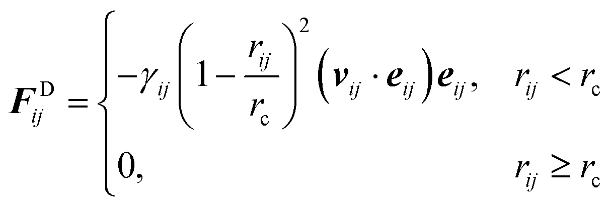
j. Similarly, the dissipative force is defined as
| |  | (2.2) |
with
vij the velocity difference vector
vij =
vi −
vj,
vi and
vj are the velocities of particles
i and
j respectively and
γij is the friction coefficient.
The stochastic random force compensates for the lost degrees of freedom after coarse-graining and along with the dissipative force acts as a thermostat for the system.
| |  | (2.3) |
where
χij is a randomly fluctuating variable that follows Gaussian statistics with zero mean and unit variance and

the square root of the integration timestep. The random weight function is related to the dissipative weight function through the relation
(2.4).
| |  | (2.4) |
The fluctuation–dissipation theorem relates the
γ and
σ parameters with the relation
σij2 = 2
γijkBT.
36 The DPD beads are topologically connected using the FENE potential with constant
,
rmax = 1.3
rc and
ro = 0.7
rc.
| | 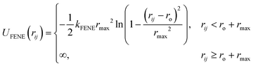 | (2.5) |
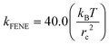
We study six combinations of aij, γij. In all cases the conservative and friction coefficients between like-particles are kept constant and are given in Table 2 where the letter P refers to the polymer beads and S to the solvent beads. We consider an a thermal solvent where aij = 25, γij = 4.5, two additional aij (15, 20) values at γij = 4.5 and two additional γij values (5, 10) at aij = 25. Varying aij and γij corresponds to modifying the solvent quality and bulk solvent viscosity, respectively. The cut-off radius is kept constant at rc = 1 in all the cases and the mass is equal for all beads (m = 1). These two quantities, together with the energy kBT = 1 set the distance, mass, and energy scales respectively.
Table 2 DPD model parameters used in the current study. P and S stand for polymer and solvent beads, respectively. The conservative, aij, and dissipative,γij, cross-terms parameters are varied as follows aij = 15, 20, 25 and γij = 4.5, 5, 10. In the polymer melts, the parameter of self-particle type interactions is varied as γii = 4.5, 5, 10 while aii = 25 always
|
a
sp
|
P |
S |
γ
sp
|
P |
S |
| P |
25 |
a
ij
|
P |
4.5 |
γ
ij
|
| S |
a
ij
|
25 |
S |
γ
ij
|
4.5 |
Since the cut-off radius of the beads (and mass) is the same regardless of the bead type, the polymer concentration in the solution is equivalent to its volume (or mass) fraction, ϕ. Thus, a concentration of cp = 0.3 is the same as volume fraction ϕ = 0.3. From now on, both notations will be used interchangeably to express the polymer concentration and/or volume fraction.
B. Structural and dynamic analysis
We calculated some static properties of the polymer chains, i.e. the end to end distance and radius of gyration, to check the consistency with previously published data.3 The end-to-end vector,  , is defined as the vector between the first and last monomer of a polymer chain and its value indicates whether the polymer is in an extended or coiled conformation.37 The Euclidean norm of
  defines the end-to-end distance, Ree. The autocorrelation function of
  gives a measure of the equilibration of the system. Usually, an exponential function of the form of eqn (2.6) is fitted to the autocorrelation function of the
  to calculate the relaxation time of the polymer chain.38
| | 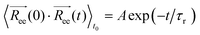 | (2.6) |
where A and τr are the fitting coefficients, τr is the relaxation time of  , and to the time origin (for an autocorrelation function example, see Fig. S5 in ESI†). We then use τr to determine the cutting point for the viscosity integral. More specifically, the final viscosity values reported below are averaged over the time interval [2τr, 3τr].13 The autocorrelation function in eqn (2.6) is calculated using multiple time origins for accuracy.
Another measure of the expansion or contraction of the polymer chain is the radius of gyration, Rg. The Rg is calculated as the average over all time frames and monomers of the distance between the chain monomers and centre of mass of the polymer chain. Monitoring Rg as a function of the polymer molecular weight (which in the present case corresponds to the number of chain beads, N, since m = 1) provides an indication of the solvent quality.
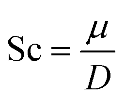
For the dynamic properties, we calculated the diffusion coefficient, D from the particles mean squared displacement, and the Schmidt number, which is a dimensionless number defined as the ratio between the kinematic viscosity, μ, and the diffusion coefficient,12
| |  | (2.7) |
In this work, we use the polymer contribution to the solution viscosity,
i.e.,
η −
ηs, for the Schmidt number calculation (
eqn (2.8))
| |  | (2.8) |
where
ρ is the density of the fluid,
η is the viscosity of the solution,
ηs is the viscosity of the solvent (
ηs = 1.1 in our case, see Fig. S1, ESI
†) and
D is the diffusion coefficient of the polymer chain. When simulating polymer melts, the viscosity used in
eqn (2.8) is the bulk viscosity
η. In this work,
D was calculated through the mean squared displacement of the chains’ centre of mass rather than the displacement of a single chain monomer.
C. Viscosity from Green–Kubo formula
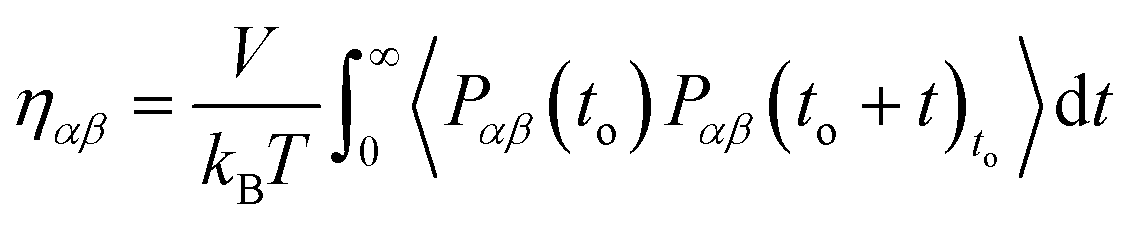
Green–Kubo (GK) relations have been extensively applied to calculate transport coefficients from DPD simulations.14,16,17,39 The relation that is used for the viscosity calculation is the integral of the pressure autocorrelation function and has the following original form:| | 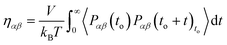 | (2.9) |
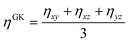
with Pαβ being the pressure tensor's off-diagonal αβ element with α, β = x, y, z. The symbol 〈…〉to refers to the evaluation of the autocorrelation function over multiple time origins to. All the off-diagonal terms of the pressure tensor are used to reduce the statistical error.38,40 Mondello and Grest have suggested using all nine pressure tensor components by adequately weighting the diagonal elements.41 Our simulations are extremely long and using only the three off-diagonal elements is sufficient to ensure good statistics.
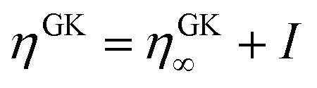
In DPD, the pressure tensor is the sum of four different contributions: the pressure due to the dissipative force, PDαβ, the conservative force, PCαβ, the random force, PRαβ and the kinetic part of the energy, PKαβ. In literature,42,43 the total pressure resulting from these four contributions is mainly used with the GK relation. However, recently it has been shown that, for high density systems (ρ > 4), if all the contributions are included within the integral of eqn (2.9), the resulting viscosity in the linear regime deviates from the value obtained by using non-equilibrium approaches.18 Thus, a revised GK formula, eqn (2.10), was suggested16,18 to achieve results comparable to non-equilibrium simulations and resolve the time reversibility issues arising from the dissipative force.16,17
| | 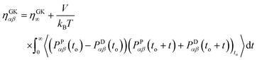 | (2.10) |
where
.
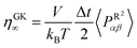
The random pressure is decorrelating instantly within the first integration time step Δt and thus its integral can be calculated by the basic geometry rule which, with the appropriate factors  , gives the instantaneous viscosity ηGK∞ in eqn (2.10).18 The instantaneous viscosity term is important for retrieving viscosity values comparable to non-equilibrium methods (see for more details ref. 18). The revised relation (2.10) gives the same viscosity as the non-equilibrium simulations irrespectively to the system density.18
Therefore, due to the extended applicability of eqn (2.10) over eqn (2.9), the relation (2.10) is used in this work. In the literature44,45 it has been shown that the highest contribution to the overall pressure autocorrelation function comes from the bonding, the conservative and kinetic forces. Thus, the pressure in eqn 2.10 includes all these terms (i.e. PPαβ = Pbondsαβ + PCαβ + PKαβ) and the total viscosity is computed as follows:
| |  | (2.11) |
To estimate the error, we follow the time decomposition method19 over 10 independent runs. This number of independent trajectories is sufficient to ensure a standard deviation lower than the mean viscosity value. In contrast to ref. 19 the viscosity cut-off point is decided according to the value of the relaxation time of the end-to-end vector, and the average viscosity is averaged over the interval [2τr, 3τr].
D. Viscosity from Einstein formula
An equivalent expression to the GK relation was derived by Helfand,21 taking into account the momentum diffusion in the system. It is an Einstein type relation and has the original form:| | 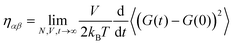 | (2.12) |
with 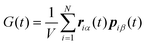 where r and p are the position and momentum of the particles, respectively and α,β = x, y, z. To overcome the discontinuity introduced by the periodic boundary conditions, an alternative formula was suggested using the integral of the pressure tensor Pαβ.24,46 So, eqn (2.12) becomes:
| | 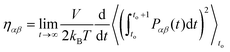 | (2.13) |
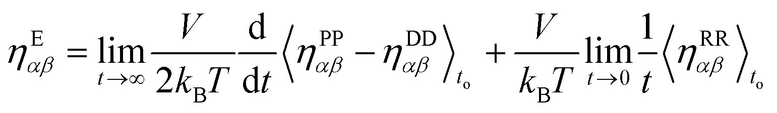
To make a direct comparison with the revised GK formula of eqn (2.10), an equivalent Einstein formula is suggested in this work, which is defined as
| |  | (2.14) |
where each term
ηAB is given as in
eqn (2.15).
| | 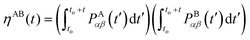 | (2.15) |
A and B are the potential, P, dissipative, D, or random, R, contributions. If A = B then it is simply the integral squared.
26
The derivation of this formula is straightforward if one starts from the equivalent relation (2.10). For the derivation, the indexes αβ indicating the directions are omitted from the general P(t) symbol. However, the derivation holds in all directions. In what follows, the symbol P refers to the total pressure due to the total force contributions. It is known that the GK and Einstein formulas are equivalent and related through the relation:
| | 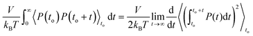 | (2.16) |
Starting from
eqn (2.10), we have
| |  | (2.17) |
Keeping only the integral terms,
I, and substituting them with the Einstein form due to
eqn (2.16):
| |  | (2.18) |
The only terms that remain from expression (2.17) are
ηPP and
ηDD since the terms
ηPD and
ηDP are equal and opposite and thus eliminate each other. Following Jung's
et al.18 derivation we define the Einstein correction term due to the random force as follows,
| |  | (2.19) |
By multiplying with the volume on each side, we get
| |  | (2.20) |
Alternatively, and in compliance with the Einstein formalism the
ηE∞ term can be also written as in
eqn (2.21),
| |  | (2.21) |
Eqn (2.21) together with
eqn (2.18) constitute the revised Einstein formalism (
eqn (2.14)). As for the GK case, the viscosity was calculated over the time interval [2
τr, 3
τr] where the system was well equilibrated, and the statistical accuracy was less than half of the viscosity value.
13
III. Results
A. Scaling of static properties
In polymer theory, the structural and dynamical properties of polymer chains scale with the number of chain monomers, N, following specific scaling laws. The scaling laws and the scaling coefficient values depend on two factors: the polymer-polymer overlap and solvent quality.47 For highly dilute solutions, where polymer-polymer overlap can be neglected, the quality of the solvent determines the magnitude of the swelling of the chain as a function of N and the radius of gyration scales with N as Rg ≈ Nv where v is the Flory exponent. If the solvent effect is unimportant (i.e., θ-conditions) v = 0.5, whilst v ≈ 0.6 indicates that the interactions between the polymer and solvent beads are energetically favourable (i.e., good solvent conditions). Upon increasing the polymer volume fraction, ϕ, above an overlap value,  , Flory screening sets in, and the Flory exponent v again becomes equal to 0.5 for all solvents. Upon increasing polymer concentration, a change in the dynamic properties mirrors the scaling of the structural ones. For dilute solutions, hydrodynamic interactions (HI) are dominant, and the Zimm model describes the scaling with N of the polymer viscosity and diffusion coefficient as η ∝ N3ν−1 and D ∝ N−ν respectively. For highly concentrated solutions and polymer melts, HI are screened, and the dynamical properties of the system follow a Rouse model where η ∝ N and D ∝ N−1.47
The crossover between the dilute and concentrated regimes does not occur suddenly, and for semidilute solutions, the polymer properties scale with the polymer volume fraction.48 Here we consider the semidilute and concentrated solutions where the polymer volume fraction is above the overlap volume fraction (ϕ*). As the scaling behaviour is fully developed for  3, we expect to see scaling exponent coefficients in better agreement with the theory in this region although the fitting of the data are reported for
  in some of our plots.
Jiang and co-workers3 have shown that for dilute and semidilute athermal polymer solutions, DPD models reproduce the correct scaling of the polymer radius of gyration (Rg) and end-to-end distance (Ree) as a function of the polymer volume fraction. Here we perform a similar scaling analysis to check the dependence of the Flory parameter value, ν, on the DPD interaction parameters. As said above, in semidilute solutions, the scaling of the Rg depends on the polymer volume fraction, ϕ, as described by eqn (3.1).47
| |  | (3.1) |
where
Rg0 is the radius of gyration of a polymer chain at infinite dilution. The values of the rescaled
Rg as a function of the rescaled volume fraction for all conservative and dissipative coefficients at
cp = 0.3 and 0.8 are presented in
Fig. 1 (left). Fitting the data with
eqn (3.1) we obtain a slope of 0.13 for the two lowest conservative parameters (
asp = 15 and 20), and 0.10 for
asp = 25. Regardless of the conservative interaction parameters, these values are in agreement with the scaling behaviour expected for real chains dissolved in good solvent for which
ν ≅ 0.59.
47 For a polymer melt,
i.e. cp = 1.0, for which excluded volume interactions are thoroughly screened, and the polymer chains follow the Rouse statistics,
Rg scales as
Rg ≈ (
N − 1)
ν, where (
N − 1) is the number of bonds, with
ν = 0.5
49,50 (
Fig. 1 (right)). In addition, no evident effect of the
γij parameter on
Rg is observed. Similar results are obtained calculating the
Ree (see ESI
† document and Fig. S3, ESI
†).
 |
| | Fig. 1 (left) The radius of gyration as a function of overlapping volume fraction. The circles stand for the polymer concentration cp = 0.3 and the squares the concentration cp = 0.8. The colours represent the different interaction parameters with black for asp = 15, blue for asp = 20, cyan for asp = 25 all with γsp = 4.5, green for asp = 25 and γsp = 5 and red for asp = 25 and γsp = 10. (right) Mean square radius of gyration as a function of polymer length for the polymer melt (cp = 1.0) simulations. | |
B. Numerical verification of revised Einstein formalism
The two equilibrium viscosity methods are initially tested on a simple DPD “water” model comprising of monomers interacting through aij = 25 and γij = 4.5 The viscosity for this model was found to be 1.1 using both methods when integrating the pressure tensor to t = 0.8 (see ESI† document and Fig. S1, ESI†). This result agrees with non-equilibrium DPD simulations carried out using Lees–Edwards boundary conditions, which calculated the zero-shear viscosity to be 1.08.
Next, we proceed with the polymer solutions, where ten independent runs are employed to evaluate the error. The average value of the viscosity obtained with both methods is comparable as these methods are numerically equivalent.22 However, their standard deviation shows a small but significant difference as the polymer length (and relaxation time) increases, with the Einstein method having a clear advantage over the GK one. To compare the two methods, the relative Mean Absolute Error (MAE) of the mean viscosity values given in eqn (3.2) is used.
| |  | (3.2) |
The symbol 〈…〉 indicates average taken over all the polymer concentrations and interaction parameters. On average, the viscosity obtained from the Einstein relation had a deviation of ∼2.4% from the value obtained by GK (
eqn (2.9)) (
Fig. 2 and 3). This difference can be attributed to numerical precision errors and does not depend on the interaction parameters.
 |
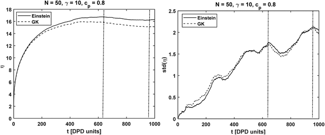
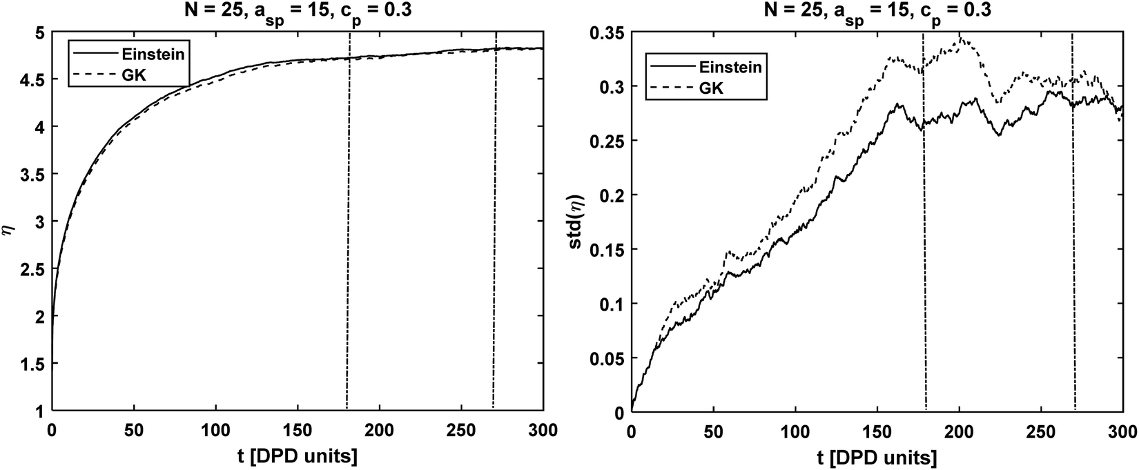
| | Fig. 2 Chain length N = 25 simulated with asp = 15, γsp = 4.5 at concentration cp = 0.3: (on the left) viscosity integral calculated with the GK and Einstein formulas. (on the right) Standard deviation calculated from 10 independent runs. The dashed vertical lines correspond to the interval [2τr, 3τr] where the viscosity was evaluated. | |
 |
| | Fig. 3 Same as Fig. 2 but for chain length N = 50 at asp = 25, γsp = 10 and at concentration cp = 0.8. | |
Although the MAE values calculated for both methods show are similar (see Fig. S2 in ESI†), the standard deviations are different. The results indicate that the Einstein method had a lower standard deviation, especially for long polymer chain lengths. Similarly to the MAE for the mean value of η shown above, we calculate the difference in standard deviations using eqn (3.3).
| |  | (3.3) |
The absolute value is omitted from the numerator to check whether the standard deviation is smaller in GK (negative MES) or Einstein relation (positive MES). As shown in
Fig. 4, for
N = 40 and 50, the standard deviation calculated using the Einstein relation can be, on average, 5–8% smaller than the standard deviation obtained using the GK formula. The difference in standard deviations is insignificant for chains with
N = 10, 25. We ascribe this result to the fact that the longer the polymer chain is, the slower is its dynamics and therefore the longer the DPD trajectory needs to be to reduce the statistical error. We observe again that the value of the MES does not depend on the interaction parameters or the polymer concentrations. Our findings are consistent with the literature which finds that the Einstein relation overcomes the effect of long temporal tails present in the pressure autocorrelation function.
30
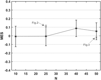 |
| | Fig. 4 Mean difference between the standard deviations calculated using the GK and Einstein relations as a function of the polymer chain lengths. The average for each polymer length, N, is taken over every polymer concentration and asp, γsp values. A negative (positive) MES value means that the standard deviation of GK is lower (higher) than the Einstein one. The standard deviations considered for this figure correspond to the time interval [2τr, 3τr]. | |
Finally, in terms of computational effort, both methods scale linearly in time as the trapezoidal rule was used for the evaluation of the integrals in both cases, which scales with ![[scr O, script letter O]](https://www.rsc.org/images/entities/char_e52e.gif) (n) where n is the number of input data points.
(n) where n is the number of input data points.
C. Scaling of dynamic properties
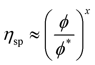
This section analyses the viscosity values calculated from the DPD simulations and verifies that our revised Einstein formula can reproduce the rheological behaviour predicted by polymer theory. The scaling of the dynamical properties with the polymer molecular weight is used in polymer physics to determine whether the polymer solutions follow the Rouse or Zimm theoretical model.3,51 The scaling of these quantities can be found using a linear fit and the value of the exponent is characteristic of the system's dynamic behaviour. In this work, we investigate the scaling of the specific viscosity ( , where ηs = 1.1 is the solvent viscosity and η is the viscosity of the solution) which is a unitless number that measures the polymer contribution to the solution viscosity.47
For semidilute polymer solutions, as with the structural properties, the scaling behaviour of the viscosity depends on the values of ϕ and ϕ*. However, if the data are normalized by the solvent viscosity (specific viscosity) and plotted against the normalized volume fractions ϕ/ϕ*, the explicit effect of the polymer length disappears and all of the data should fall onto a single master curve.52Fig. 5 (left) shows that indeed the specific viscosities calculated from the DPD simulations fit the same master curve. The scaling of the specific viscosity with the polymer concentration predicted by the theory is given by the following expression:
| |  | (3.4) |
where

and
ν is the Flory exponent. In athermal and
θ-solvent (
ν ≅ 0.5), the exponent
x ≅ 2.0 and the viscosity is predicted to grow as the square of the polymer concentration. In a good solvent where we expect hydrodynamic interactions to be dominant
ν ≅ 0.6 and
x ≅ 1.25.
47 We fit the data obtained from the lower reduced molar fraction

simulations and the higher ones
separately. In both cases we observe that the exponent
x is approximately 1.3 regardless of the interaction parameters, but the data fits the theoretical prediction better when

.
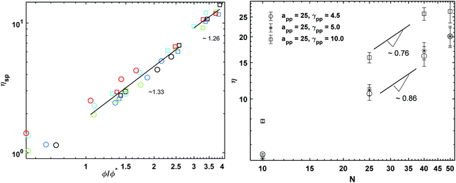 |
| | Fig. 5 (left) Specific viscosity as a function of reduced molar fraction for polymer concentrations cp = 0.3 and 0.8. The circles stand for the polymer concentration cp = 0.3 and the squares the concentration cp = 0.8. The colours represent the different interaction parameters with black for asp = 15, blue for asp = 20, cyan for asp = 25, green for γsp = 5 and red for γsp = 10. (right) Bulk viscosity as a function of polymer length for polymer melts. | |
Next, we check the scaling of the diffusion coefficients, D. In the cases of cp = 0.3 and 0.8, the diffusion should follow the relation (3.5) and the value of the exponent, w, indicates the absence or dominance of HI.
| | 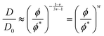 | (3.5) |
where
w ≈ 1 indicates
θ-solvent while
w ≈ 0.54 good solvent conditions and
D0 refers to the diffusion coefficient at infinite dilution. In agreement with the viscosity scaling analysis, the exponents calculated from the values of
D are closer to the predictions for good solvent than
θ-solvent conditions (
Fig. 6, left). It should be noted that in the cases with

both excluded volume and hydrodynamic interactions must be considered.
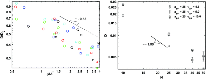 |
| | Fig. 6 (left) Normalized diffusion coefficient as a function of reduced molar fraction for polymer concentrations cp = 0.3 and 0.8. The circles stand for the polymer concentration cp = 0.3 and the squares the concentration cp = 0.8. The colours represent the different interaction parameters with black for asp = 15, blue for asp = 20, cyan for asp = 25, green for γsp = 5 and red for γsp = 10. (right) Diffusion coefficient as a function of polymer length calculated for the polymer melts. | |
The viscosity data calculated from the melt simulations are reported in Fig. 5 (right). The friction parameter, γij, affects the value of the viscosity and the scaling exponents. We find that the scaling of viscosity is below the expected theoretical prediction, η ∼ N whilst the diffusion data reported in Fig. 6 (right), follows the Rouse theory, i.e., D ∼ N−1 the latter despite the chain lengths of some of models are quite short.53 This difference among the viscosity and diffusion exponents has been observed previously for polymer melts modelled with similar DPD parameters as the ones employed here. In particular, Posel et al.53 showed that the scaling of viscosity severely deviates from the scaling of the self-diffusion coefficient as the FENE spring constant increases. The authors point out that as the values of kFENE increases, the elastic contributions to the pressure tensor vanish and the viscous contributions dominate. It may therefore be expected that the scaling behaviour of the viscosities of models with high kFENE and relative short chain lengths (as those simulated here) may depart from the Rouse theory which considers only elastic contributions. Here we see the same disagreement between the D, η exponent values, with a kFENE = 40.0 which is higher than the bond stiffness coefficients studied in the work of Posel et al.53 However, the deviation we observe is not as severe as it is in ref. 53 Calculating the characteristic ratio, CN, (Fig. S4 in ESI†) for the melts, we also observe that, despite the higher kFENE used here, our DPD chains are more flexible than some of those modelled by Posel et al.53,54 probably due to the different rmax employed.
D. Schmidt number
The Schmidt numbers (Sc) calculated for the polymer solutions and melts using eqn (2.7) are reported in Fig. 7. It is known from the literature55 that the Schmidt number for a DPD representation of an ideal gas (i.e., aij = 0) can be approximated by eqn (3.6).| | 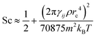 | (3.6) |
which indicates a parabolic dependence of Sc on the friction parameter, γij. Although we are not in an ideal gas case, this parabolic dependence seems to be followed in the present case as well, and the data points are fitted well by a function of the form 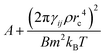 where A, B are fitting coefficients (for the fittings, see Fig. S6 in ESI†).
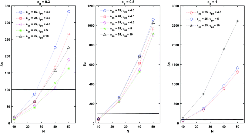 |
| | Fig. 7 Schmidt number at different polymer concentrations and interaction parameters. Sc values above the horizontal line are characteristic of liquid systems, while below this line, the system is in the gaseous regime. | |
From Fig. 7, it appears evident that Sc depends on both the interaction parameters and the length of the chain, N. Irrespectively of the value of γsp, the lowest value of Sc is observed for cp = 0.3 and asp = 25. For this conservative coefficient, the chains create “blobs” with a small radius of gyration (Rg) which diffuse faster within the solvent than an extended polymer chain, leading to a low Sc number. In this work, D refers to the diffusion of the chain's centre of mass rather than the diffusion of a single chain monomer. This definition is expected to increase the value of Sc compared to using the diffusion of single chain monomers.55
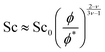
Additionally, we can build a master curve for the Schmidt number plotting its normalized value (Sc/Sc0) against the reduced polymer molar fraction (Fig. 8). The data can be fitted with eqn (3.7) which is obtained using the definition the Schmidt number (eqn (2.7)) and the scaling equations for the viscosity and diffusion coefficient (eqn (3.4) and (3.5))
| |  | (3.7) |
where

for good solvents and

for
θ-conditions. As observed for the viscosity exponent coefficient, the fitting value of

, which suggests that we are closer to good solvent conditions. The term Sc
0 here is the Schmidt number calculated for infinite dilution,
i.e.,

.
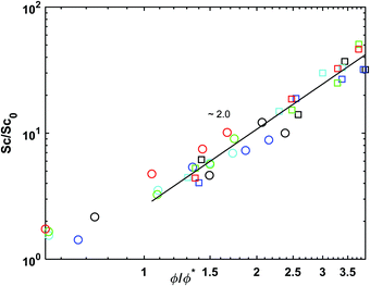 |
| | Fig. 8 Normalized Schmidt number as a function of reduced molar fraction for polymer concentrations cp = 0.3 and 0.8. The circles stand for the polymer concentration cp = 0.3 and the squares the concentration cp = 0.8. The colours represent the different interaction parameters with black for asp = 15, blue for asp = 20, cyan for asp = 25, green for γsp = 5 and red for γsp = 10. | |
Finally, the ability of DPD to simulate liquid phases is evident by the fact that Sc > (102). which is indicative of a liquid.12,56 The ability of DPD to simulate liquids was debated in the past55 mainly because in DPD simulations typically Sc ∼ (1). Here we observe that the order of Sc is increased by a factor of 102 for the lowest polymer concentration, cp = 0.3 and up to 103 in polymer melts, cp = 1. With the correct choice of conservative interaction parameters, the modelling of high Schmidt number liquids using DPD is possible.
IV. Summary
The performance of Einstein–Helfand formalism was examined in this work in the presence of stochastic and dissipative forces and compared with the revised DPD Green Kubo (GK) formula suggested by Jung and Schmid.18 A revised Einstein–Helfand formula was proposed for calculating the zero-shear viscosity from equilibrium DPD simulations and was applied in this work to calculate the viscosity of polymer solutions of different concentrations, cp = 0.3, 0.8, 1.0 and chain lengths N = 10, 25, 40, 50. In order to numerically verify our revised Einstein formalism a comparison with the revised GK formula suggested by Jung and Schmid18 was carried out, and the transport properties of the systems were studied.
The viscosities were evaluated over three different conservative and friction coefficients using the time decomposition method19 to estimate the errors. For both approaches, the viscosity was calculated as an average in the interval [2τr, 3τr] with τr the chain relaxation time. The average viscosity value and the standard deviations from Einstein and GK were the same over 10 independent runs, however a difference of 5–8% was observed in the standard deviations for chain lengths N = 40, 50 in favour of the Einstein relation, while the average value of viscosity was the same for both methods. This difference is attributed to the error propagation in the long chains. This result indicates that the Einstein relation has higher statistical accuracy than the Green–Kubo formula at early time intervals. Additionally, we performed a scaling analysis on the polymer melts and solutions' dynamical properties and found that the scaling laws predicted by the theory are well reproduced. Our results indicate that our revised Einstein–Helfand relation can confidently be used to calculate the zero-shear viscosity for complex, slow relaxing fluids.
Data availability statement
Codes written in C++ can be found in the repository github.com/MariaPanoukidou/zero-shear-viscosity for both methodologies applied in this work. The data that support the findings of this study are available from the corresponding author upon request.
Conflicts of interest
There are no conflicts to declare.
Acknowledgements
The Engineering and Physical Sciences Research Council and Unilever's financial support (grant reference EP/N509280/1) is gratefully acknowledged. The authors would like to acknowledge the assistance given by Research IT and the use of the Computational Shared Facility at The University of Manchester. We would like to thank Prof. J. B. Ávalos (Rovira i Virgili University) and Prof. A. Masters (The University of Manchester) for the fruitful conversations on the Einstein methodology for the viscosity calculations.
References
- A. Prhashanna, S. A. Khan and S. B. Chen, Colloids Surf., A, 2016, 506, 457–466 CrossRef CAS.
- H. Droghetti, I. Pagonabarraga, P. Carbone, P. Asinari and D. Marchisio, J. Chem. Phys., 2018, 149, 184903 CrossRef PubMed.
- W. Jiang, J. Huang, Y. Wang and M. Laradji, J. Chem. Phys., 2007, 126, 1–27 Search PubMed.
- M. Panoukidou, C. R. Wand, A. Del Regno, R. L. Anderson and P. Carbone, J. Colloid Interface Sci., 2019, 557, 34–44 CrossRef CAS PubMed.
- A. Vishnyakov, M. T. Lee and A. V. Neimark, J. Phys. Chem. Lett., 2013, 4, 797–802 CrossRef CAS.
- R. L. Anderson, D. J. Bray, A. Del Regno, M. A. Seaton, A. S. Ferrante and P. B. Warren, J. Chem. Theory Comput., 2018, 14, 2633–2643 CrossRef CAS PubMed.
- C. R. Wand, M. Panoukidou, A. Del Regno, R. L. Anderson and P. Carbone, Langmuir, 2020, 36, 12288–12298 CrossRef CAS.
- A. Boromand, S. Jamali and J. M. Maia, Comput. Phys. Commun., 2015, 196, 149–160 CrossRef CAS.
- J. A. Backer, C. P. Lowe, H. C. J. Hoefsloot and P. D. Iedema, J. Chem. Phys., 2005, 122, 154503 CrossRef CAS PubMed.
- R. Pasquino, N. Grizzuti, P. Carbone, H. Droghetti, D. Marchisio and S. Mirzaagha, Soft Matter, 2019, 15, 1396–1404 RSC.
- D. Pan, J. Hu and X. Shao, Mol. Simul., 2016, 42, 328–336 CrossRef CAS.
- J. Zhao, S. Chen and N. Phan-Thien, Mol. Simul., 2018, 44, 797–814 CrossRef CAS.
- A. David, A. De Nicola, U. Tartaglino, G. Milano and G. Raos, J. Electrochem. Soc., 2019, 166, B3246–B3256 CrossRef CAS.
- A. Chaudhri and J. R. Lukes, Phys. Rev. E: Stat. Nonlinear, Soft Matter Phys., 2010, 81, 1–11 CrossRef.
- H. Noguchi and G. Gompper, EPL, 2007, 79, 36002 CrossRef.
- M. H. Ernst and R. Brito, EPL, 2006, 73, 183 CrossRef CAS.
- M. H. Ernst and R. Brito, Phys. Rev. E: Stat. Nonlinear, Soft Matter Phys., 2005, 72, 1–11 CrossRef PubMed.
- G. Jung and F. Schmid, J. Chem. Phys., 2016, 144, 204104 CrossRef.
- Y. Zhang, A. Otani and E. J. Maginn, J. Chem. Theory Comput., 2015, 11, 3537–3546 CrossRef CAS PubMed.
- D. M. Heyes, E. R. Smith and D. Dini, J. Chem. Phys., 2019, 150, 174504 CrossRef CAS PubMed.
- E. Helfand, Phys. Rev., 1960, 119, 1–9 CrossRef.
-
J. M. Haile, Molecular dynamics simulation, elementary methods, Wiley, 1992, vol. 288 Search PubMed.
- S. Viscardy, J. Servantie and P. Gaspard, J. Chem. Phys., 2007, 126, 184512 CrossRef CAS PubMed.
- B. J. Alder, D. M. Gass and T. E. Wainwright, J. Chem. Phys., 1970, 53, 3813–3826 CrossRef CAS.
- P. Español, Phys. Rev. E: Stat. Nonlinear, Soft Matter Phys, 2009, 80, 1–13 CrossRef.
- K. Meier, A. Laesecke and S. Kabelac, J. Chem. Phys., 2004, 121, 3671–3687 CrossRef CAS.
- K. Meier, A. Laesecke and S. Kabelac, J. Chem. Phys., 2005, 122, 0–9 CrossRef CAS.
- S. Hess and D. J. Evans, Phys. Rev. E: Stat. Physics, Plasmas, Fluids, Relat. Interdiscip. Top., 2001, 64, 6 Search PubMed.
- S. Hess, M. Kröger and D. Evans, Phys. Rev. E: Stat. Physics, Plasmas, Fluids, Relat. Interdiscip. Top., 2003, 67, 4 Search PubMed.
- C. Nieto-Draghi, J. B. Ávalos and B. Rousseau, J. Chem. Phys., 2003, 119, 4782–4789 CrossRef CAS.
- M. E. Cates, J. Phys., 1988, 49, 1593–1600 CrossRef.
- M. Lísal, J. K. Brennan and J. B. Avalos, J. Chem. Phys., 2011, 135, 204105 CrossRef PubMed.
- J. B. Gibson and K. Chen, Int. J. Mod. Phys. C, 1999, 10, 241–261 CrossRef.
- M. A. Seaton, R. L. Anderson, S. Metz and W. Smith, Mol. Simul., 2013, 39, 796–821 CrossRef CAS.
- E. Moeendarbary, T. Y. Ng and M. Zangeneh, Int. J. Appl. Mech., 2009, 01, 737–763 CrossRef.
- P. Espanol, Phys. Rev. E, 1995, 52, 1734–1742 CrossRef CAS.
-
M. P. Allen and D. J. Tildesley, Computer Simulation of Liquids, Oxford University Press, 2017 Search PubMed.
- J. T. Padding and W. J. Briels, J. Chem. Phys., 2001, 114, 8685–8693 CrossRef CAS.
- A. Chaudhri and J. R. Lukes, Int. J. Numer. Methods Fluids, 2009, 60, 867–891 CrossRef.
- D. Nevins and F. J. Spera, Mol. Simul., 2007, 33, 1261–1266 CrossRef CAS.
- M. Mondello and G. S. Grest, J. Chem. Phys., 1997, 106, 9327–9336 CrossRef CAS.
- M. Mouas, J. G. Gasser, S. Hellal, B. Grosdidier, A. Makradi and S. Belouettar, J. Chem. Phys., 2012, 136, 094501 CrossRef PubMed.
- R. Kubo, J. Phys. Soc. Jpn., 1957, 12, 570–586 CrossRef.
- K. S. Kim, C. Kim, G. E. Karniadakis, E. K. Lee and J. J. Kozak, J. Chem. Phys., 2019, 151, 1–22 Search PubMed.
- E. Zohravi, E. Shirani and A. Pishevar, Mol. Simul., 2018, 44, 254–261 CrossRef CAS.
- P. E. Smith and W. F. van Gunsteren, Chem. Phys. Lett., 1993, 215, 315–318 CrossRef CAS.
-
M. Rubinstein and R. H. Colby, Polymer physics, Oxford University Press, Oxford, 2003 Search PubMed.
- A. Jain, B. Dünweg and J. R. Prakash, Phys. Rev. Lett., 2012, 109, 1–4 Search PubMed.
- R. H. Colby, Rheol. Acta, 2010, 49, 425–442 CrossRef CAS.
-
P.-G. De Gennes, Scaling concepts in polymer physics, Cornell University Press, 1979 Search PubMed.
- T. Taddese, D. L. Cheung and P. Carbone, ACS Macro Lett., 2015, 4, 1089–1093 CrossRef CAS.
- E. Raspaud, D. Lairez and M. Adam, Macromolecules, 1995, 28, 927–933 CrossRef CAS.
- Z. Posel, B. Rousseau and M. Lísal, Mol. Simul., 2014, 40, 1274–1289 CrossRef CAS.
- F. Lahmar, C. Tzoumanekas, D. N. Theodorou and B. Rousseau, Macromolecules, 2009, 42, 7485–7494 CrossRef CAS.
- R. D. Groot and P. B. Warren, J. Chem. Phys., 1997, 107, 4423 CrossRef CAS.
- C. Gualtieri, A. Angeloudis, F. Bombardelli, S. Jha and T. Stoesser, Fluids, 2017, 2, 17 CrossRef.
Footnote |
| † Electronic supplementary information (ESI) available. See DOI: 10.1039/d1sm00891a |
|
| This journal is © The Royal Society of Chemistry 2021 |
Click here to see how this site uses Cookies. View our privacy policy here. 
 Open Access Article
 This Open Access Article is licensed under a
  ,
Charlie R.
Wand
,
Charlie R.
Wand


 the square root of the integration timestep. The random weight function is related to the dissipative weight function through the relation (2.4).
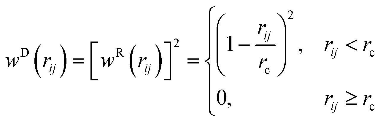
 , rmax = 1.3rc and ro = 0.7rc.
 , is defined as the vector between the first and last monomer of a polymer chain and its value indicates whether the polymer is in an extended or coiled conformation.37 The Euclidean norm of
  defines the end-to-end distance, Ree. The autocorrelation function of
 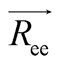 gives a measure of the equilibration of the system. Usually, an exponential function of the form of eqn (2.6) is fitted to the autocorrelation function of the
  to calculate the relaxation time of the polymer chain.38
 , and to the time origin (for an autocorrelation function example, see Fig. S5 in ESI†). We then use τr to determine the cutting point for the viscosity integral. More specifically, the final viscosity values reported below are averaged over the time interval [2τr, 3τr].13 The autocorrelation function in eqn (2.6) is calculated using multiple time origins for accuracy.


 .
.
 , gives the instantaneous viscosity ηGK∞ in eqn (2.10).18 The instantaneous viscosity term is important for retrieving viscosity values comparable to non-equilibrium methods (see for more details ref. 18). The revised relation (2.10) gives the same viscosity as the non-equilibrium simulations irrespectively to the system density.18

 where r and p are the position and momentum of the particles, respectively and α,β = x, y, z. To overcome the discontinuity introduced by the periodic boundary conditions, an alternative formula was suggested using the integral of the pressure tensor Pαβ.24,46 So, eqn (2.12) becomes:


 , Flory screening sets in, and the Flory exponent v again becomes equal to 0.5 for all solvents. Upon increasing polymer concentration, a change in the dynamic properties mirrors the scaling of the structural ones. For dilute solutions, hydrodynamic interactions (HI) are dominant, and the Zimm model describes the scaling with N of the polymer viscosity and diffusion coefficient as η ∝ N3ν−1 and D ∝ N−ν respectively. For highly concentrated solutions and polymer melts, HI are screened, and the dynamical properties of the system follow a Rouse model where η ∝ N and D ∝ N−1.47
 3, we expect to see scaling exponent coefficients in better agreement with the theory in this region although the fitting of the data are reported for
 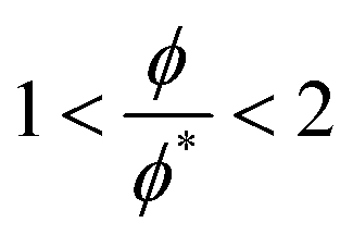 in some of our plots.


 , where ηs = 1.1 is the solvent viscosity and η is the viscosity of the solution) which is a unitless number that measures the polymer contribution to the solution viscosity.47
 and ν is the Flory exponent. In athermal and θ-solvent (ν ≅ 0.5), the exponent x ≅ 2.0 and the viscosity is predicted to grow as the square of the polymer concentration. In a good solvent where we expect hydrodynamic interactions to be dominant ν ≅ 0.6 and x ≅ 1.25.47 We fit the data obtained from the lower reduced molar fraction
  simulations and the higher ones
 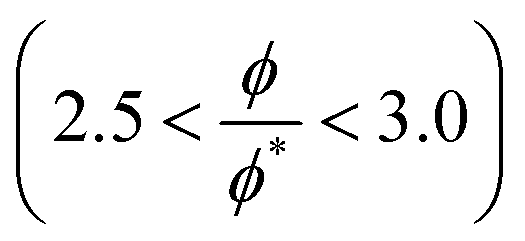 separately. In both cases we observe that the exponent x is approximately 1.3 regardless of the interaction parameters, but the data fits the theoretical prediction better when
  .
.


 both excluded volume and hydrodynamic interactions must be considered.


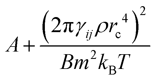 where A, B are fitting coefficients (for the fittings, see Fig. S6 in ESI†).


 for good solvents and
  for θ-conditions. As observed for the viscosity exponent coefficient, the fitting value of
  , which suggests that we are closer to good solvent conditions. The term Sc0 here is the Schmidt number calculated for infinite dilution, i.e.,
  .
.
