Structural transitions at electrodes, immersed in simple ionic liquid models

Abstract

We used a recently developed classical Density Functional Theory (DFT) method to study the structures, phase transitions, and electrochemical behaviours of two coarse-grained ionic fluid models, in the presence of a perfectly conducting model electrode. Common to both is that the charge of the cationic component is able to approach the electrode interface more closely than the anion charge. This means that the cations are specifically attracted to the electrode, due to surface polarization effects. Hence, for a positively charged electrode, there is competition at the surface between cations and anions, where the latter are attracted by the positive electrode charge. This generates demixing, for a range of positive voltages, where the two phases are structurally quite different. The surface charge density is also different between the two phases, even at the same potential. The DFT formulation contains an approximate treatment of ion correlations, and surface polarization, where the latter is modelled via screened image interactions. Using a mean-field DFT, where ion correlations are neglected, causes the phase transition to vanish for both models, but there is still a dramatic drop in the differential capacitance as proximal cations are replaced by anions, for increasing surface potentials. While these findings were obtained for relatively crude coarse-grained models, we argue that the findings can also be relevant in “real” systems, where we note that many ionic liquids are composed of a spherically symmetric anion, and a cation that is asymmetric both from a steric and a charge distribution point of view.

---

1 Introduction

Research on ionic liquids (ILs) has increased dramatically in recent years. ILs have many interesting properties, perhaps the most obvious of which is the fact that they have remarkably low melting points, considering their expected strong intermolecular interactions. For most ILs, a contributing factor is a geometric “mismatch” between the ions, which makes it sterically difficult for them to arrange into a stable crystalline lattice.

ILs have high charge density, and their electrostatic coupling strength is usually quite strong. This means that they have a high electrostatic screening capacity, which is one of the reasons why many of them are interesting candidates for electrochemical applications, such as electric double layer capacitors.^1–4 This has meant that not all the experimental research in the field has been applied in nature. There have also been many theoretical studies, including detailed atomistic simulations,^5–7 as well as more coarse-grained modelling, focusing on the fundamental properties of these fascinating fluids.^8–15 Probably the simplest coarse-grained model that has been utilized for this purpose is the so-called restricted primitive model (RPM). While the RPM has been a popular and useful model for aqueous electrolyte solutions,^16,17 it has also been used in studies of ILs.¹⁸ In this model, any solvent (absent in the case of neat ILs) only enters implicitly, via a relative dielectric constant. The ions are modelled as hard spheres, with a common diameter d. A charge is embedded at each hard-sphere centre, and for most models of ILs this charge is usually monovalent. It should, however, be noted that for realistic IL densities at room temperature, the RPM will likely freeze, as its symmetrical nature generates a strong propensity to form ordered structures.

We noted earlier that steric “mismatch” is one of the reasons why many ILs have a low melting temperature. So, in order to form a stable liquid under ambient conditions, the RPM needs to be suitably modified to reflect this asymmetry in structure. Spohr and Patey introduced a model wherein the ions are described as charged Lennard-Jones particles. Those authors focused on how bulk properties responded to changes of charge and size asymmetry.^19,20 Patey and Lindenberg investigated further extensions, where the cations carry two partial charges, one of which is displaced from the centre of the Lennard-Jones particle.²¹ Other modifications of the RPM have focused on fundamental mechanisms at the electrode–fluid interface. Bazant utilized a lattice model, ensuring a saturation limit, to investigate overscreening and crowding effects of ILs at charged surfaces.¹² Kornyshev,²² Fedorov^23,24 and Lamperski^25,26 have systematically considered size and shape asymmetries, for modifications of the RPM. Lu et al.^27–29 have investigated bulk and electrochemical properties of the asymmetric RPM (ARPM), which is identical to the RPM, except that the charges on anions and cations are both displaced a certain (equal for both) distance from the hard-sphere centre.

In this work, we shall use primarily classical density functional theory (DFT) to explore the properties of a model, that closely resembles the ARPM. However, instead of displacing the originally centrally placed charge in all ions, we will retain an RPM-like central charge for the anions, while the cationic charge is displaced a distance b from the hard-sphere centre. We shall denote this as the generalized Asymmetric RPM, (GARPM). In common with the ARPM, the GARPM will only introduce one additional parameter, to the original RPM. Furthermore, a large displacement b will lower the melting point of the bulk fluid – a general property shared with the ARPM. However, we expect that the propensity of the GARPM to form ion pairs is considerably lower than the ARPM. In other words, an anion can in principle interact quite strongly with two cations, whereas it will favour a single partner with ARPM architecture. One could argue that the GARPM has the advantage of a somewhat closer resemblance to typical ILs, since these commonly are composed of a roughly spherical anion, and an oligomeric cation, with an asymmetrically placed charge.

Using isobaric bulk simulations, we will first establish a value of b that generates a fluid phase with a density typical of ILs, under ambient conditions. This GARPM will be used in subsequent investigations, focusing on electrochemical properties, where a conducting electrode is immersed in the IL fluid. We will then utilize classical DFT that is able to (albeit approximately) deal with both ion–ion correlations, and surface polarization using a screened image charge approach.

As we shall demonstrate below, the DFT predicts a possible structural phase separation at the electrode interface, in these systems. This phase separation results from competition, at a positively charged electrode, between cations and anions. The cations are strongly attracted because of their ability to allow their charge to be closer to the electrode surface, placing them close to the dielectric interface. This leads to a strong self-image interaction. On the other hand, the anions are attracted by the overall positive electrode charge.

A significant advantage of the DFT is that, since we obtain the appropriately minimized grand potentials, we have an essentially complete description of the phase separation. An interesting consequence of this phase separation is a divergent differential capacitance in the potential range over which the transition occurs.

Given the rather simple competition mechanism that underlies the phase transition, we have also investigated this phenomenon with an even simpler model. Specifically, we use the RPM at an elevated temperature (to prevent freezing) where we introduce adsorption asymmetry (as described above), by allowing the cations to “penetrate” the electrode surface by some distance δ. This will generate a stronger attractive self-image interaction for cations at the electrode surface, in a manner that is qualitatively analogous to what we find for the GARPM. We shall denote this simpler model the “wall penetrating cation” RPM, (or RPM(wpc)). As expected the RPM(wpc) displays a similar behaviour to the GARPM, according to our DFT predictions, i.e. a phase transition occurs at some threshold applied voltage.

It should be noted that phase transitions at, or inside, electrodes have been suggested for other models of similar systems in the past.^13,15,30,31 Szparaga et al.¹³ investigated ionic liquid + solvent systems, displaying a thin-thick (prewetting) transition, whereby an IL-rich layer formed at the electrode surface. This transition could, for temperatures above the wetting temperature but below the surface critical point, be regulated by the electrode potential. The transition was accompanied by a divergence of the differential capacitance at the potential where coexistence of phases occurs. Ref. 30 describes a somewhat related IL + solvent system, where dilute-concentrated phase transitions could be generated inside (model) nanoporous electrodes. While there are some apparent similarities with these transitions, and those we find in this work, we emphasize that we do not observe a prewetting, or capillary-condensing, transition in our systems. Instead, our systems display surface transitions that emerge from a liquid bulk and are therefore structural in nature. From the perspective of the mean-field theory used here, this type of transition is indicated by a change in the layering of the fluid, given that in-plane structure is not explicitly accounted for. In our model it is largely driven by a difference in the distance of closest approach of anions and cations to the dielectric discontinuity of the electrode. This means cations are able to polarize the conducting electrode more strongly, leading to a much larger self-image interaction. Our system bears a closer resemblance to the one studied by Merlet et al.¹⁵ who simulated a coarse-grained IL model (as opposed to our simplified model) in the presence of metallic electrodes. They observed a capacitance peak that grew with system size, indicating the possibility of a phase transition in a macroscopic system. If so, the transition would be of structural nature, and mechanistically similar to those we observe here. In their systems they see a drastic change in both the layering as well as in-plane structure. This notwithstanding, we raise the caveat that the conjectured phase transition is based on a system-size scaling argument and it is possible that the indicative divergence in the capacitance will prove to be finite upon approach to the thermodynamic limit. There is also some suggestion in their observations that this transition may occur at both positive and negative potentials, whereas the nature of the transition in our system is clearly asymmetric. Finally, we note that Lee and Perkin³¹ used a phenomenological theory to investigate potential-induced phase transitions at electrodes. They noted some features that are generally true for phase transitions in these kinds of systems, such as a diverging differential capacitance at the transition, but it is difficult to make specific comparisons with the results found in the work described here.

2 Model and theory

All charges are embedded in a hard sphere, with a common diameter d. In this work, as in our previous investigations of the ARPM, we have set d = 5.0 Å. For anions, this charge is centrally located in the hard sphere, but for cations, it is displaced a distance b from the centre. This means that our extension amounts to one additional parameter, as compared with the RPM. In our earlier work on the ARPM,^27,28 where both ions have a displaced charge, we used a b value of 1.0 Å. This generated a fluid at room temperature and pressure, with a liquid-like density of about 2.9–3.0 M, which is typical for an IL. This value for b in the ARPM gave a distance of closest approach between anions and cations of 3.0 Å. Guided by this, we have used b = 2.0 Å for the GARPM used in this work, which gives the same distance of closest approach between ion pairs. Bulk NPT simulations have verified that this also gives rise to a fluid, with a density of about 3M, at room temperature, and a pressure of 1 bar. This was our target bulk density for all DFT calculations and simulations in this work. The bulk density of the RPM(wpc) was set identical to that used for the GARPM, i.e. 3M, although the temperature was set to 900 K, in order to prevent crystallization.

The RPM(wpc) model was developed as an even simpler alternative to the GARPM, sharing the latter's tendency to preferentially adsorb cations at a neutral conducting surface. This is achieved by allowing the cations to approach the plane of dielectric discontinuity more closely than the hard-sphere radius, which is the case for anions. This facilitates a strong cationic self-image interaction across the dielectric interface, in a manner that is qualitatively similar to what we expect in a GARPM fluid. In all other respects the RPM(wpc) is identical to the RPM.

The GARPM and RPM(wpc) are both very coarse-grained representations of ILs. Nevertheless, there are some aspects of typical imidazolium-based ILs that provide a qualitative rationale of how these models are constructed. We expect that the ring-like shape of the aromatic part where the net cation charge is mainly located, will admit close proximity of the cationic charge to a polarizing (conducting) surface, as obtained via simple orientational optimization. Typical anions, however, tend to have a roughly spherical shape, with less (or no) option for orientational optimization.

Electrochemical and structural properties were investigated in a slit geometry, with the ionic fluid confined between two parallel and perfectly conducting, flat electrodes. The surfaces have an infinite extension in the (x, y) plane, and distances along the z direction are measured from the plane of dielectric discontinuity (z = 0) at the left wall. The right wall is placed with its plane of dielectric discontinuity at z = h. This separation is chosen to be large enough to ensure close to bulk-like conditions midway between the surfaces. The confined fluid is assumed to be in equilibrium with a bulk solution, with a density of about 3.0M.

The GARPM and RPM(wpc) models are illustrated, in the proximity of a (model) electrode surface, in Fig. 1.

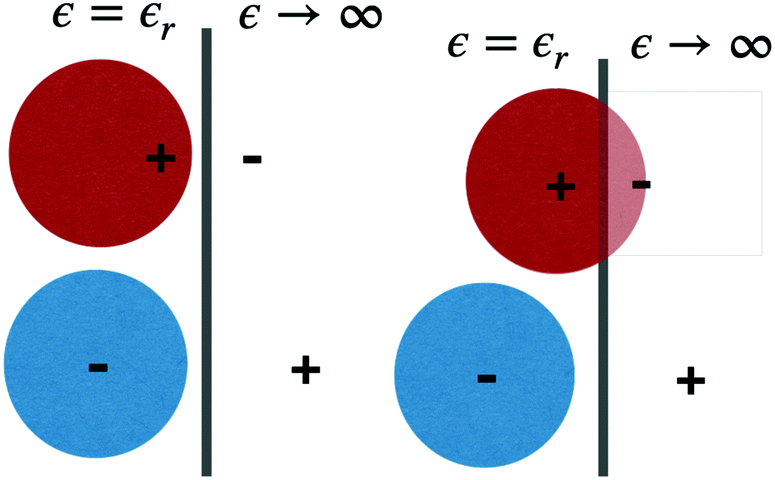Fig. 1 An illustration of our model ions, near the surface of a perfectly conducting electrode. Image charges are also indicated. Left graph: the GARPM model. Right graph: the RPM(wpc) model.

The Coulomb interaction, u^γδ_el(r), between two charges of valency Z_γ and Z_δ, located a distance r from each other, is:

where β is the inverse thermal energy, ε₀ is the permittivity of vacuum and ε_r is the relative dielectric constant, accounting for screening from degrees of freedom that are not explicitly accounted for in the model. The Bjerrum length, l_B, is defined as:Since our model lacks explicit treatment of electron polarization, we shall model that contribution implicitly, by setting ε_r = 2. We will utilize image charges to capture electrode polarization effects, with the electrode being regarded as a perfect conductor. The hard wall potential will normally prevent the ion hard-sphere centres from approaching the plane of dielectric discontinuity closer than δ = 0.5d. However, as described above for the cations in the RPM(wpc) model, this distance is smaller and we set it to δ = 0.1d.

2.1 Bulk isobaric simulations

We calculated the density of the GARPM model using Monte Carlo simulations in the isobaric (NPT) ensemble at 1 bar and 298 K. The system consisted of 400 ion pairs and was equilibrated for 10⁷ steps, 10⁹ configurations were used to determine the volume average. The electrostatic interactions were calculated using Ewald summation, with a real space cutoff of 25 Å and 512 reciprocal space vectors. The splitting parameter was set to , where L_i = 61 Å denotes the side of the initial (cubic) simulation box. Tinfoil boundary conditions were used, corresponding to a surrounding medium with infinite relative permittivity. The volume of the simulation box was found to oscillate around a value corresponding to a bulk density of around 3M.

The outcome of the simulation was a bulk density of about 3M.

2.2 Density functional theory, DFT

We shall recapitulate the density functional theory, which is a slightly modified version of the formulation introduced in an earlier work, on the ARPM.²⁹ In the same work, predictions of the DFT were validated, by comparisons with simulation data on identical systems.

2.2.1 The iPB approximation of image interactions. We emphasize that our treatment is limited to monovalent ions, although a generalization is straightforward. The self-interaction, V_self, of a monovalent ion, with its own image charges, can be written as:where l_max is a chosen upper limit of a sum with, strictly speaking, an infinite number of terms. The attractive potential from V_self is counteracted by a screening effect, since our “tagged” ion will (on average) be preferentially surrounded by an opposite charge, the image of which generates a repulsion. The range of the ionic atmosphere is expected to be of order ∼κ⁻¹, where κ is the inverse Debye–Hückel screening length in the bulk:where n_i is the density of species i. Hence, the attractive self-image term for each ion is accompanied by a repulsive contribution, stemming from the oppositely charged atmosphere.

In our previous work,³² we suggested a simple approach to estimate the counterion screening. With the conducting surface being located at z = 0, a positive charge at z will be attracted by its negative self-image, at −z, with the same (x, y) coordinates as the real charge. We assume that this image charge is neutralized by a uniformly charged circular disc of radius R_d, centred at the position of the image charge and oriented parallel with the surface. This can be viewed as a projection of the cylindrically symmetric ion atmosphere onto the plane containing the self-image charge, generating a charged circular disc, at −z.

We let P_vdW(0) denote the zero frequency van der Waals (vdW) pressure between two flat conducting surfaces. In the presence of a dielectric medium, that separates two semi-infinite conducting slabs, this can be written as:^33,34

where ζ(n) is the Riemann zeta function. The effect of intervening salt in these systems is to screen P_vdW(0), resulting in a non-algebraic decay.³³ Dielectric fluctuations are ignored in the Primitive Model, so the ionic contribution to the surface pressure neglects P_vdW(0), which means that the electrostatic surface pressure must be corrected by a long-ranged term, which is equal to −P_vdW(0).^33,34

We shall utilize this fact to determine the size, R_d of our counterion disc. This radius will thus be quantified by requiring perfect cancellation of the van der Waals (vdW(0)) interaction. This will have three relevant consequences:

• The sum {self-image charge + disc charge} is zero, ensuring that the total image potential drops to zero when the original charge is far away from the surface.

• The potential contribution from {the self-image charge + disc charge} is analytic.

• The correct zero frequency vdW interaction between neutral conducting surfaces is reproduced (by construction).

The interaction (in units of thermal energy) between a tagged ion at z, and the disc image, at a single surface, can be written as: 2πl_B[(R_d² + 4z²)^1/2 − 2z]. Hence the total image potential, V_image, with two conducting surfaces separated by h, becomes:

This potential can then be directly imported to a density functional formulation of the Poisson–Boltzmann theory, to give an image-corrected version, which we denote, iPB. Given that we only need to calculate the total image potential once, for each DFT calculation, we can use a very large number of reflections, at a modest computational expense. In this work we have used one thousand reflections, ensuring fully converged sums.

It is straightforward to demonstrate that this approach will generate an interaction pressure between two conducting surfaces that decays as h⁻³, in agreement with the expected zero frequency van der Waals attraction.²⁹ Previous work^29,32 have demonstrated the following quantitative relationship: R_d ≈ 2.85/κ, which is tantalizingly close to . This is an empirically based relation, that still awaits formal confirmation. Nevertheless, repeated tests, for a wide range of different conditions, have verified that this choice will indeed perfectly oppose P_vdW(0), at a long range.

Note that our polarization approximations are limited to a mean-field level, i.e. fluctuation modes generated by the non-uniform structuring of ions at the surfaces, are neglected. Other approximate treatments of image interactions have been proposed. For instance, Kandûc et al.³⁵ introduced a “dressed ion” approach, where monovalent ions, in highly asymmetric z:1 salt solutions, were effectively integrated out. However, this approach seems less well suited to the 1 : 1 salt systems considered in this work.

2.2.2 Mean-field DFT. Our final theory will include an approximate treatment of ion correlations, but let us at this stage start with a simpler DFT formulation, where electrostatics is handled at the mean-field level. However, even our “mean-field” DFT (approximately) includes excluded volume effects, so it is not analogous to a Poisson–Boltzmann (PB) formulation. An important consequence is that the mean-field DFT will display surface saturation, in contrast to PB based predictions.

A mean-field treatment of all Coulomb interactions means that electrostatics are handled at the non-linear level.^36,37 The cations of our GARPM will be handled by polymer DFT,^38–40 at the dimer level. In other words, a cation is treated as a heterogeneous dimer, where a neutral hard core centre is bonded to a point-like charge. We approximate excluded volume effects using a weighted density functional,⁴¹ based of the “Generalized Flory-Dimer” (GFD) approach.^37,42 We limit ourselves to systems where b = 2.0 Å (cations only).

2.2.3 A brief recapitulation of polymer DFT. The anions of our GARPM are simply spherical, and the cations only have dimer character. We shall nevertheless first provide a rather general description of a polymer mixture, which in principle permits a broader range of systems to be treated. This will then be specialized to our systems, and we will provide explicit iterative formulas for the cations.

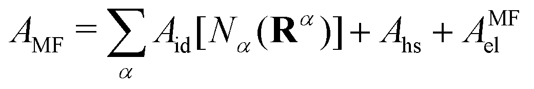
We let α identify be an oligomeric species. The configuration of an r-mer α molecule can be compactly written as R^α = r^α₁, r^α₂,…., r^α_r. The Helmholtz free energy functional (A_MF) is, at this mean-field stage, given by a sum of ideal (A_id), hard-sphere (A_hs) and mean-field electrostatic (A^MF_el) terms:

The ideal free energy is just a direct sum of the separate contributions from each of the constituent species,where Φ^α_b(R^α) describes the bonding within the α species, whereas V^(α,i)_ext(r_i) is an applied external potential from the electrode surfaces.

By integrating interactions between charge densities, we arrive at the electrostatic contribution to the free energy, A^MF_el. Note that we thereby also neglect any short-range constraints on these energy integrals due to the hard spheres in which the charges are embedded. The lack of ion correlations (at this level of theory) effectively leads to an overestimated repulsion between ions of like charge, although this is, to some degree, balanced by an overestimated attraction between unlike charges (due to the lack of a hard-core truncation). We will address this issue by adding a separate correlation term, as well as by including a steric adjustment to the short-range part of the Coulomb interaction between opposite charges.

The mean-field free energy term can be written as:

where V_image denotes a contribution from image charges within the (perfectly conducting) electrodes.

Our fluids are in chemical equilibrium with a surrounding bulk solution, which is accounted for by a transformation to the grand potential, Ω_MF:

where N_i is the number of particles of type i between the electrodes, μ_i is the chemical potential of i, and ψ_D is the Donnan potential,⁴³ which is adjusted so as to ensure electroneutrality. The grand potential, Ω_MF, is then minimized with respect to the densities.

2.2.4 Explicit iterative formulas, in the slit geometry. We will now specialize the treatment, since the ions of this study have a simple molecular architecture. In fact, only the cations of the GARPM have a dimer character, with other ions being spherically symmetric. We will therefore focus on iteration formulas for the cations.

We use indices “1” and “+” for the cation hard-sphere centre, and cation charge centre, respectively. The connection between the centre and the charge is modelled by an internal bond that is rotationally flexible, but with a fixed length b. For a cation, this means that where δ(x) is the Dirac delta function.

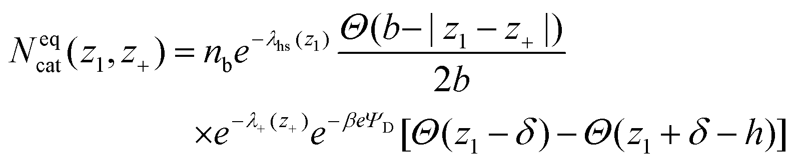
The two conducting electrode surfaces are placed at z = 0, and z = h, forming a slit. These walls are separated widely enough (h = 60 Å) to ensure that they can be regarded as two isolated electrodes, immersed in a bulk solution. A mean-field integration along the (x, y) dimensions parallel with the surfaces, leaves only z-dependent quantities. Denoting the bulk salt concentration by n_b, we obtain the equilibrium distribution of cations, N^eq_cat(z₁, z₊), by minimizing the free energy:³⁸

where Θ(x) is the Heaviside step function, and is a Boltzmann weight at z, originating from electrostatic interactions:while λ_hs is the excess hard-sphere (excluded volume) contribution:The equilibrium density of positive charge at z₊, n₊(z₊), is then obtained from:Similarly, the equilibrium density of hard sphere centers at z₁, n₁(z₁):The analogous, but simpler, treatment of spherically symmetric ions should be obvious.

2.2.5 Correlation-corrected DFT. As we will demonstrate below, the ordering transitions that are the focus of this work, will not be predicted at the mean-field level of our theory, i.e. by the level of theory presented thus far. We will now introduce approximate correlations between charges, starting with those that carry the same sign. Like-charged correlations generate a region of depleted density, surrounding some “tagged” ions. This effectively creates “Coulomb holes”, and we will borrow relations obtained within the so-called “Debye–Hückel hole” theory, DHH, proposed by Nordholm and co-workers.^44–46 We add a correlation term to Ω_MF, arriving at Ω_DHH, which is a grand potential that (approximately) includes effects from correlations between ions of like charge:Here, μ^α_DHH is obtained by differentiating f_DHH at the bulk density of component α. According to the DHH theory, the correlation free energy per particle, i.e. f_DHH[n̄_α(r)] is given bywhere ξ = [1 +cn̄^1/2_α]^1/3 and . Here, n̄ denotes a coarse-grained density, where the range of integration H is approximated by the DHH hole in the bulk:with

H = κ⁻¹[(1 + (3Γ)^3/2)^1/3 − 1]. (19)

where we have introduced a dimensionless coupling strength, Γ:where a = (4πn^d_b/3)^−1/3.

2.2.6 Correlations between opposite charges. So far, we have only included correlations between ions of like charge. They are indeed the main cause of typical ion correlation phenomena, such as overcharging, or the attraction between like-charged surfaces. In fact, in dilute and less strongly coupled systems, such as most aqueous solutions, the inclusion of like-charge correlations may well prove sufficient. However, in the dense systems studied here, such an “unbalanced” account often generates predictions of a too cohesive fluid, where the bulk pressure is negative. This is related to the fact that the mean-field theory allows complete penetration by opposite charge densities, i.e. their mutual steric repulsion is neglected. We shall here utilize the same approximation as in our previous work on the ARPM, and include an effective hard sphere exclusion correlation, so that the interaction between opposite charges, A^±_el now reads:

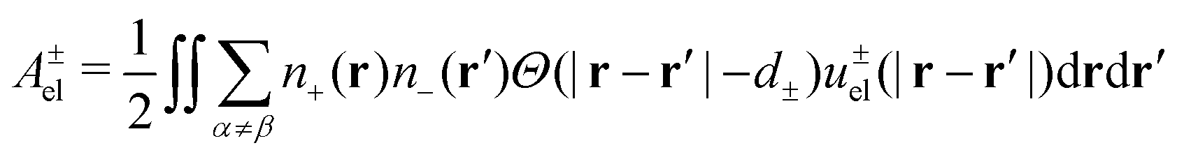
The diameter, d_±, of the effective exclusion hole, is adjusted to a value for which the bulk pressure becomes positive, and of the order of 1–10 bar. The full correlation functional, Ω, is obtained from Ω_DHH by replacing the mean-field expression for interactions between opposite charges by A_el^±, as given in eqn (21). Finally, we let ω denote the grand potential per unit area.

3 Results

We will start by highlighting DFT predictions for our GARPM systems, subsequently proceeding to the even simpler RPM(wpc). Obvious advantages of our DFT approach over computer simulations include computational speed, noise-free data, and the direct calculation of the free energy.

3.1 GARPM

Let us start by presenting predictions of how the surface potential, Ψ_S, varies with the surface charge density, σ_S. Note that in the DFT calculations, ω is minimized at a fixed value of σ_S. We can then establish Ψ_S in two independent ways. The most straightforward route is an extrapolation of Ψ(z) to the z = 0 plane, where Ψ(z) itself is obtained by integrating the charge density profile.⁴⁷ The surface potential can also be found via the Legendre transformation relation: Ψ_S = ∂ω/∂σ_S. Such independent relations are quite useful, since they serve as a, usually sensitive, test of the numerical calculations. Data obtained for the two approaches are presented in Fig. 2, where it is obvious that they agree. We can also identify two separate phases, labelled “A” and “B”, the regimes of which are separated by an unstable region, where Ψ_S decreases as σ_S increases. This is analogous to the unstable portion of the classic van der Waals pressure versus density of a single-component fluid below the critical point. In that case a uniform and constant density plays the role of the order parameter. In the case considered here, the surface charge density is the order parameter. If it is assumed to be constant over the electrode, an unstable portion of the corresponding free energy functional can eventuate. The horizontal red dashed line indicates the potential, Ψ^(c)_s, which is the value where A and B phases coexist. Above Ψ^(c)_S, A is the stable phase, whereas B is stable below this value. As in the van der Waals fluid, the line satisfies an equal area constraint for the enclosed regions of the potential curve above and below the line. If the potential Ψ^(c)_S ≈ 0.36 V, was applied in an experimental realization of our model, the stable system would consist of two surface phase regions on the electrode. In the A-region, the surface charge density would have the value σ_S = σ^(c)_S(A) ≈ 0.0028 e Å⁻², with the corresponding A structure of the adjacent liquid. It would coexist with a B-region, where σ_S = σ^(c)_S(B) ≈ −0.012 e Å⁻². Separating the two regions would be a 1-dimensional interface which would contribute a line energy which grows proportionally with the square root of the electrode surface. This line energy is infinite in the thermodynamic limit, which means the transition is first-order.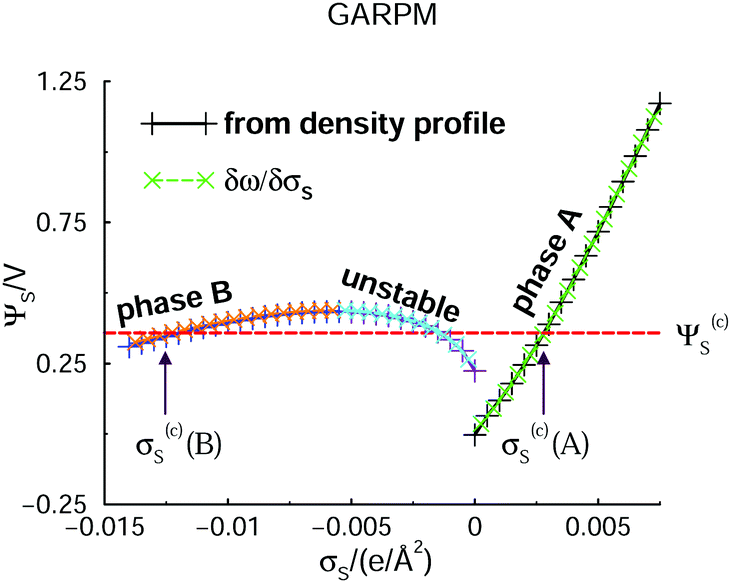

Fig. 2 DFT predictions for how the electrode surface potential varies with the surface charge density, in the presence of the GARPM fluid. The surface potential is evaluated in two equivalent, but independent ways: from integrations of the charge density profiles (solid curves with plus signs), or from discrete derivatives of the grand potential per unit area with respect to the surface charge density (dashed curves with crosses). Results from both methods are provided, as indicated in the legend. One can identify two different phases, “A” and “B”, with the latter being stable for surface potentials below Ψ^(c)_S ≈ 0.36 V. Phase A is stable above Ψ^(c)_S, which thus identifies the value at which the two phases coexist. The value of Ψ^(c)_S can be obtained from the Legendre-transformed grand potential, see Fig. 3, and is provided as a dashed horizontal (red) line. There are also regions where phases A and B are metastable. In the region where the curve has a negative slope, i.e. where Ψ_S drops as σ_S increases, the system is unstable. The spinodal can thus be found from the points at which the tangent is horizontal.

Another observation worth pointing out is that, while the ARPM and GARPM are rather closely related, the reduced symmetry of the latter has a substantial impact on electric double layer behaviours. We recall that all double layer properties of the ARPM are symmetrical with respect to zero surface charge density, i.e. a neutral surface.

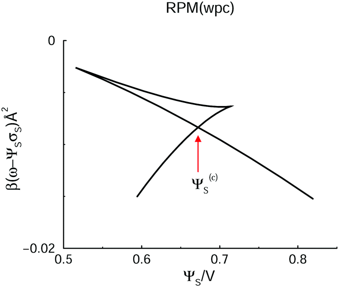
In a typical experimental situation, a voltage is applied, which results in some average surface charge density. Hence, it is instructive to make a Legendre transformation of our grand potential per unit area, ω, to arrive at another grand potential, ω − Ψ_Sσ_S, for which the surface potential is the natural variable. In Fig. 3, we have plotted how this grand potential varies with Ψ_S, for our GARPM system.

Fig. 3 The variation of the Legendre-transformed grand potential, ω − Ψ_Sσ_S, with applied voltage, for the GARPM system. The system displays a phase separation, and the red arrow marks the point at which the two phases (A and B) coexist. This identifies the value of Ψ^(c)_S, which was indicated by a dashed red line in Fig. 2.

The region where the phase transition occurs is more apparent in this case, and we can easily identify the crossing of the two branches, at about 0.36 V, where the two phases, i.e. A and B, coexist. This is the way in which we established the dashed horizontal red line that marks Ψ^(c)_S, in Fig. 2. The crossing is marked by a red arrow, in Fig. 3. In passing, we note that the DFT predicts that phase separation may occur also in a system with reduced electrostatic coupling, as achieved by doubling the dielectric constant, to ε = 4. However, the demixing regime is then substantially diminished, i.e. they are then rather close to a “critical value” of ε. This is explicitly illustrated in the Appendix.

In Fig. 4, we present density profiles for the coexisting A and B phases (at about Ψ_S = 0.36V).

Fig. 4 Charge density profiles (n₊ and n₋) for coexisting A and B phases, at Ψ_S ≈ 0.36 V.

The structural differences are quite large, and from a mere visual inspection, it is far from obvious that the surface potential is the same for both phases. In a “real” system, one might end up with macroscopic regions of each phase, separated by interfacial boundaries. Note that the surface charge density differs between the two phases, which underlines the importance to consider the experimental “boundary condition” of a constant applied voltage. It is also worth noting how the cations in phase B are able to utilize their strong self-image attraction (i.e. surface polarization) to generate a very strong density peak at the surface. This leads to overcharging, and the primary anionic density peak is actually higher for phase B than for phase A, despite the fact that the bare surface charge density of the former is negative. As we progress further away from the electrode, the strong screening from near-surface ion layers ensures a rapid approach to bulk-like properties.

As mentioned earlier, the differential capacitance, C_D will diverge for a system that undergoes a phase transition, at the electrode surface. This is obvious from its definition, C_D ≡ ∂σ_S/∂Ψ_S, combined with the fact that the phases (A and B) coexist at a common voltage, but with a different surface charge density. Hence, a transition from one phase to the other effectively amounts to a sudden change of σ_S without any change of Psi_S, resulting in a diverging C_D. This was discussed in some detail in ref. 13 and 30, and also mentioned in ref. 15.

The transition is illustrated in Fig. 5, where the vertical line marks the equilibrium crossover between the phases. Note how an increased voltage along the B branch will see a dramatic increase of the capacitance, upon entering the metastable regime. In practice, one will likely encounter hysteresis effects in such a system. Another interesting observation, in Fig. 5, is how the overall C_D level of the B branch, which is cation-rich at the electrode surface, is about 5 times higher than the capacitance of the A branch. This obviously results from the strong proximity of the cationic charge to the electrode interface.

Fig. 5 Differential capacitance of the GARPM. The vertical line marks the surface potential, Ψ^(c)_S, at which the A and B phases coexist, i.e. parts of the metastable regions are also included in the graph. Note that B is the stable phase below Ψ^(c)_S, whereas A is the equilibrium phase for higher potentials.

3.2 RPM(wpc)

Encouraged by the interesting structural response found for a fluid as simple as the GARPM, we decided to scrutinize an even simpler model – the RPM(wpc).

The variation of the surface potential with surface charge density is given in Fig. 6. Similarly to the GARPM system, we observe an unstable regime, with a negative slope, which clearly indicates a demixing regime. However, in contrast to the GARPM, the curve is continuous. This signifies the fact that, contrary to the GARPM, DFT calculations of the RPM(wpc) under these conditions, will never produce two different solutions (of which only one is stable) for a given surface charge density.

Fig. 6 Variation of the electrode surface potential with surface charge density, in the presence of the RPM(wpc) fluid. The notation is analogous to the one used in Fig. 2, with the exception that we here refrain from explicit identifications of the full A-phase, B-phase, and unstable regimes.

The corresponding Legendre-transformed grand potential, ω − Ψ_Sσ_S, is shown in Fig. 7. Again, the analogy with the GARPM is clear, i.e. the inherent ability of the electrode surface to specifically attract cations leads to an anion–cation competition at the surface for positive potentials. This ultimately leads to the formation of two structurally different phases. The point where the curve crosses itself identifies the condition at which these two phases coexist.

Fig. 7 The variation of the Legendre-transformed grand potential, ω − Ψ_Sσ_S, with applied voltage, for the RPM(wpc) system.

The differential capacitance of the RPM(wpc) system is given in Fig. 8. The overall appearance of the C_D curve is quite similar to the one for the GARPM, albeit displaced to higher voltages. In this system, the ratio between the C_D levels of the (stable) B and A branches is about 6–7, which again highlights the important role that the proximity between fluid charge and electrolyte surface (plane of dielectric discontinuity) has. In an experimental system, or a theoretical model with atomistic resolution, this might correspond to the charge of a spherical anion (BF₄⁻, say) being “buried”, whereas the charge of an asymmetric cation (BMIM⁺, say) is more “exposed” (by an optimized molecular orientation) to the electrode surface.

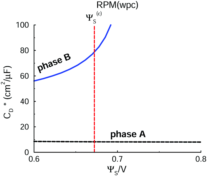Fig. 8 Differential capacitance of the RPM(wpc). The notation is analogous to that used in Fig. 5. We emphasize that B is the stable phase below Ψ^(c)_S, whereas A is the equilibrium phase for higher potentials. This means that the part of the B-curve that is above Ψ^(c)_S indicates metastable conditions (analogous for the A-curve below Ψ^(c)_S).

3.2.1 Phase diagram. It is of interest to work out how the coexisting phases merge, as the temperature is increased towards a critical value. In Fig. 9, we plot the phase diagram, above 900 K, for the RPM(wpc) model. The surface charge density for coexisting A and B phases clearly merge to a critical point, at a temperature slightly above 1400 K. Since our DFT neglects fluctuations, we anticipate d − 1 mean-field critical behaviours, similar to mean-field treatments of other kinds of surface transitions, such as prewetting. In passing, we note that our RPM(wpc) system was obviously located “deep” into the demixing regime, with a critical temperature being more than 50% higher than the investigated value.

Fig. 9 Phase diagram of the RPM(wpc) system.

3.2.2 Mean-field results. Let us finally explore the DFT predictions that result if electrostatics is treated at the mean-field level. The option to “remove” ion correlations is an attractive feature of the density functional approach, as it allows scrutiny on the specific role of these correlations, but also an insight on how an otherwise similar, but less strongly coupled system might behave.

Differential capacitance curves for the GARPM and RPM(wpc) systems, as predicted by mean-field DFT, are given in Fig. 10.

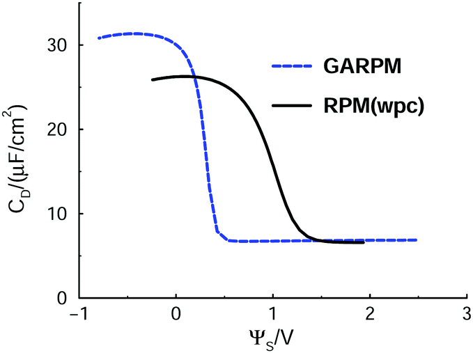Fig. 10 Differential capacitance of the GARPM and RPM(wpc), according to a version of DFT, where electrostatics is handled at the mean-field level, i.e. where all accounts of ion correlations have been removed from the original formulation.

As expected, the phase transition is lost, but the impact of the model asymmetries, compared to an RPM reference, is still quite pronounced. In fact, one observes a “trace” of the transition found in a more strongly coupled system, as manifested by a dramatic drop of C_D for an increased potential, in a narrow regime where the cation-dominated electric double layer is replaced by an anion-dominated layer. For the GARPM system, the capacitance of the cation-rich double-layer is nearly 5 times higher than that afforded by an anion-rich layer. For the RPM(wpc), the corresponding ratio is about 4. These differences are naturally caused by the ability of the cations to approach the electrode interface more closely than the anions.

4 Conclusions

We have explored some electrochemical and structural behaviours of two very simple and coarse-grained IL models: the GARPM and the RPM(wpc). In fact, the RPM(wpc) is perhaps more appropriately viewed as a model of a molten salt. An important aspect, from an electric double layer point of view, that is shared by both models, is the ability of the cationic charge to approach the electrode interface more closely than its anionic analogue. Remarkably enough, this is, according to our DFT, enough to generate a phase transition. This transition originates from a competition, at positive applied voltages between surface-polarization attracted cations, and surface charge attracted anions, at the interface. We invoke an approximate treatment of ion correlations in our DFT formulation, and an earlier study demonstrated that this generates a reasonably accurate account of these effect.²⁹ The electrode is modelled as a perfect conductor, and surface polarization is handled by an approximate image charge treatment, that has been tested and validated in earlier work.³² The phase transition vanishes with a mean-field treatment of electrostatics, but the competition will then still generate a dramatic drop of the differential capacitance, as an increased voltage transforms a cation-dominated electric double layer to one where the electrode surface is enriched by anions. We hope to corroborate these transitions by simulations, in future work.

Conflicts of interest

There are no conflicts to declare.

Appendix: less strongly coupled GARPM

Here, we demonstrate that phase separation also may occur in systems in which the electrostatic coupling is weaker. In Fig. 11, we compare grand potential predictions, for the GARPM with a dielectric constant of 2 (our reference value), 4, and 6.

Fig. 11 The variation of the Legendre-transformed grand potential, ω − Ψ_Sσ_S, with applied voltage, for the GARPM system. Results are shown for systems with dielectric constants of ε = 2 (same as in Fig. 3), ε = 4, and ε = 6.

The possibility for phase separation at a higher dielectric constant is evident, but it is also clear that a weaker coupling leads to a smaller demixing regime. In fact, the tiny demixing regime for ε = 6 indicates that this is close to the critical value. This prediction may prove useful for future simulation studies, where a strong electrostatic coupling usually leads to sluggish behaviours, and slow convergence. The DFT predictions suggest that one might be able to establish phase separation, also in systems with weaker coupling.

Acknowledgements

J. F. acknowledges financial support from the Swedish Research Council.

Notes and references

1. P. Simon and Y. Gogotsi, Nat. Mater., 2008, 7, 845–854.
2. Y. Bai, Y. Cao, J. Zhang, M. Wang, R. Li, P. Wang, S. M. Zakeeruddin and M. Grätzel, Nat. Mater., 2008, 7, 626–630.
3. S. Ito, S. M. Zakeeruddin, P. Comte, P. Liska, D. Kuang and M. Grätzel, Nat. Photonics, 2008, 2, 693–698.
4. M. Armand, F. Endres, D. R. MacFarlane, H. Ohno and B. Scrosati, Nat. Mater., 2009, 8, 621–629.
5. M. R. Lynden-Bell, M. G. Del Papolo, G. A. Tristan, J. Kohanoff, C. G. Hanke, J. B. Harper and C. C. Pinilla, Acc. Chem. Res., 2007, 40, 1138.
6. R. Lynden-Bell and T. Youngs, J. Phys.: Condens. Matter, 2009, 21, 424120.
7. J. Vatamanu, M. Vatamanu, O. Borodin and D. Bedrov, J. Phys.: Condens. Matter, 2016, 28, 464002.
8. A. A. Kornyshev, J. Phys. Chem. B, 2007, 111, 5545–5557.
9. D. Roy and M. Maroncelli, J. Phys. Chem. B, 2010, 114, 12629–12631.
10. S. Kondrat, N. Georgi, M. V. Fedorov and A. A. Kornyshev, Phys. Chem. Chem. Phys., 2011, 13, 11359–11366.
11. J. Forsman, C. E. Woodward and M. Trulsson, J. Phys. Chem. B, 2011, 115, 4606–4612.
12. M. Z. Bazant, B. D. Storey and A. A. Kornyshev, Phys. Rev. Lett., 2011, 106, 046102.
13. R. Szparaga, C. E. Woodward and J. Forsman, J. Phys. Chem. C, 2012, 116, 15946–15951.
14. C. Merlet, M. Salanne and B. Rotenberg, J. Phys. Chem. C, 2012, 116, 7687–7693.
15. C. Merlet, D. T. Limmer, M. Salanne, R. van Roij, P. A. Madden, D. Chandler and B. Rotenberg, J. Phys. Chem. C, 2014, 118, 18291–18298.
16. S. Lamperski and D. Henderson, Mol. Simul., 2011, 37, 264–268.
17. D. Henderson, S. Lamperski, Z. Jin and J. Wu, J. Phys. Chem. B, 2011, 115, 12911–12914.
18. D.-E. Jiang, Z. Jin and J. Wu, Nano Lett., 2011, 11, 5373–5377.
19. H. Spohr and G. Patey, J. Chem. Phys., 2008, 129, 064517.
20. H. V. Spohr and G. Patey, J. Chem. Phys., 2010, 132, 154504.
21. E. K. Lindenberg and G. N. Patey, J. Chem. Phys., 2015, 143, 024508.
22. A. A. Kornyshev, J. Phys. Chem. B, 2007, 111, 5545–5557.
23. M. V. Fedorov and A. A. Kornyshev, J. Phys. Chem. B, 2008, 112, 11868–11872.
24. M. Fedorov, N. Georgi and A. Kornyshev, Electrochem. Commun., 2010, 12, 296–299.
25. S. Lamperski, M. Kaja, L. B. Bhuiyan, J. Wu and D. Henderson, J. Chem. Phys., 2013, 139, 054703.
26. S. Lamperski, J. Sosnowska, L. B. Bhuiyan and D. Henderson, J. Chem. Phys., 2014, 140, 014704.
27. H. Lu, B. Li, S. Nordholm, C. E. Woodward and J. Forsman, J. Chem. Phys., 2016, 145, 234510.
28. H. Lu, S. Nordholm, C. E. Woodward and J. Forsman, J. Phys.: Condens. Matter, 2018, 30, 074004.
29. H. Lu, S. Nordholm, C. E. Woodward and J. Forsman, J. Chem. Phys., 2018, 148, 193814.
30. R. Szparaga, C. E. Woodward and J. Forsman, J. Phys. Chem. C, 2013, 1728–1734.
31. A. A. Lee and S. Perkin, J. Phys. Chem. Lett., 2016, 7, 2753–2757.
32. R. Szparaga, C. E. Woodward and J. Forsman, Soft Matter, 2015, 11, 4011–4021.
33. J. Mahanty and B. Ninham, Dispersion forces, Academic Press, 1976.
34. R. Kjellander and S. Marčelja, Chem. Phys. Lett., 1987, 142, 485–491.
35. M. Kandûc, A. Naji, J. Forsman and R. Podgornik, Phys. Rev. E: Stat., Nonlinear, Soft Matter Phys., 2011, 84, 011502.
36. S. Nordholm, Aust. J. Chem., 1984, 37, 1.
37. J. Forsman, J. Phys. Chem. B, 2004, 108, 9236.
38. C. E. Woodward, J. Chem. Phys., 1991, 94, 3183.
39. J. Forsman and C. E. Woodward, J. Chem. Phys., 2004, 120, 506.
40. J. Forsman and C. E. Woodward, Macromolecules, 2006, 39, 1269.
41. S. Nordholm, M. Johnson and B. C. Freasier, Aust. J. Chem., 1980, 33, 2139.
42. K. G. Honnell and C. K. Hall, J. Chem. Phys., 1991, 95, 4481–4501.
43. F. G. Donnan, Z. Elektrochem. Angew. Phys. Chem., 1911, 17, 572.
44. S. Nordholm, Chem. Phys. Lett., 1984, 105, 302.
45. R. Penfold, S. Nordholm, B. Jönsson and C. E. Woodward, J. Chem. Phys., 1990, 92, 1915.
46. R. Penfold and S. Nordholm, J. Chem. Phys., 1991, 95, 2048.
47. L. Mier-y Teran, S. Suh, H. S. White and H. T. Davis, J. Chem. Phys., 1990, 92, 5087.

---