
 Open Access Article
 This Open Access Article is licensed under a
 Creative Commons Attribution 3.0 Unported Licence
Steering droplets on substrates using moving steps in wettability†
Josua
Grawitter
 * and
Holger
Stark
* and
Holger
Stark
Technische Universität Berlin, Institut für Theoretische Physik, Straße des 17. Juni 135, 10623 Berlin, Germany. E-mail: josua.grawitter@physik.tu-berlin.de; holger.stark@tu-berlin.de
First published on 7th January 2021
Abstract
Droplets move on substrates with a spatio-temporal wettability pattern as generated, for example, on light-switchable surfaces. To study such cases, we implement the boundary-element method to solve the governing Stokes equations for the fluid flow field inside and on the surface of a droplet and supplement it by the Cox–Voinov law for the dynamics of the contact line. Our approach reproduces the relaxation of an axisymmetric droplet in experiments, which we initiate by instantaneously switching the uniform wettability of a substrate quantified by the equilibrium contact angle. In a step profile of wettability the droplet moves towards higher wettability. Using a feedback loop to keep the distance or offset between step and droplet center constant, induces a constant velocity with which the droplet surfs on the wettability step. We analyze the velocity in terms of droplet offset and step width for typical wetting parameters. Moving instead the wettability step with constant speed, we determine the maximally possible droplet velocities under various conditions. The observed droplet speeds agree with the values from the feedback study for the same positive droplet offset.
1 Introduction
If a droplet can go uphill and move in response to light, where are the limits of its motility? In their seminal experiment, Chaudhury and Whitesides1 demonstrated that liquid droplets can be driven up a tilted plane against gravity by chemically treating the plane so it gradually becomes more wettable with height. Later, Ichimura et al.2 showed that sessile droplets start moving in response to gradients in wettability, which are produced by a photo-chemical reaction. These experiments essentially demonstrated an early use of structured light to create motion on the micron scale, an approach which has recently become the focus of intense research.3–5 Light-driven fluid motion6–10 is an especially favorable control mechanism because of its high precision and controllability through the established experimental methods in optics.11 Notably, it can be used in combination with or as an alternative to electrowetting techniques.12 Precise control of fluid motion is foundational for advanced lab-on-a-chip devices,13–15 as well as self-cleaning surfaces,16,17 and printing with sub-droplet precision.4,18Recently, significant advances toward light-switchable substrates with large wettability gradients have been made.19 First, Zhu et al.20 demonstrated light-induced droplet motion on a substrate modified by azobenzene–calix[4]arene where the equilibrium contact angle, as a measure for wettability, ranged from 33° to 110°. Second, several groups21,22 have designed arrays of micropillars made from light-switchable polymer material. Switching the pillars between an upright and buckled shape offers the possibility to reversibly switch the substrate into a superhydrophobic state where wettability is vanishingly small.
In this article we implement the boundary-element method23–28 to solve the full three-dimensional equations of Stokes flow in order to study droplet motion induced by non-uniform and dynamic wettability patterns. In particular, we apply our method to moving step profiles in wettability and explore the limits of droplet motion induced by such wettability gradients, i.e., we determine the maximally possible droplet speeds under various conditions.
Literature provides two research lines relevant to us. First, in two articles McGraw et al. implemented the boundary element method to gain insights into the internal flow fields of axisymmetric droplets.29,30 They combined theory and experiment to study how droplets relax towards their new equilibrium shape on a substrate after an instantaneous change in the spatially uniform wettability. Second, Glasner31 implemented the boundary element method to study the dynamics of droplets placed on substrates with static but non-uniform wettability profiles. The study employed a quasi-static approximation where the gas–liquid interface of the droplet is always assumed to be equilibrated w.r.t. to the shape of the contact line. In a very recent example of the same research line, Savva et al.32 extended Glasner's method by describing the gas–liquid interface with the so-called thin-film approximation for Stokes flow for highly wettable substrates.
Our approach goes beyond both research lines because it combines dynamic and spatially non-uniform wettability patterns and thereby offers the possibility to study continuous droplet motion. It explores more widely the research avenue recently opened in an experiment by Gao et al.33 who continuously drove a droplet up a tilted plane using a thermally induced wettability gradient that moved along with the droplet.
We apply our method to investigate a droplet surfing on a moving step in wettability in two ways: first, by positioning the droplet at a constant distance or offset from the center of the wettability step using a feedback loop, we induce a self-regulated motion of the droplet. Its velocity depends subtly on the properties of the wettability step and its offset from the droplet. From this first study we obtain typical values for the velocity with which a droplet can be moved in a wettability step. Second, by letting the wettability step approach the droplet with a constant speed, we find that up to the feedback-regulated velocity the droplet is carried along by the wettability step, while above this velocity the droplet is left behind. The study also helped us to understand the role of convexity in designing wettability profiles to induce steady droplet motion.
The article is structured as follows. We present the theory of the boundary element method and its implementation in Section 2. Our numerical approach is validated in Section 3 by studying a sessile droplet on a substrate with homogeneous wettability. We study the droplet surfing on a wettability step using a feedback loop in Section 4 and by moving the wettability step with a constant speed in Section 5. Finally, in Section 6 we present our conclusions.
2 Boundary element method for dynamic wetting: theory and implementation
We consider a liquid droplet sitting on a solid substrate with switchable wettability (Fig. 1). The droplet is bounded by two surfaces: its interface with the substrate and its free interface with the gaseous atmosphere. The intersection where the surfaces meet is the contact line, which is the three-phase contact line where liquid, solid, and gaseous phase meet. Our aim is to describe the droplet motion in response to wettability changes of the substrate. The current section provides the methodology to treat such a situation. To move the droplet, we need to calculate the fluid velocity field on the droplet surfaces using the boundary element method (Section 2.1) and the velocity of the contact line using the Cox–Voinov law (Section 2.2). After discretizing the droplet surface (Section 2.3), we can then move each vertex point r(i) along the surface normal n(i) (Section 2.4). We also implement a method to keep the volume fixed (Section 2.5) and mesh optimization to avoid acute-angled triangles in the surface mesh (Section 2.6). Finally, we nondimensionalize our equations and introduce relevant material parameters (Section 2.7).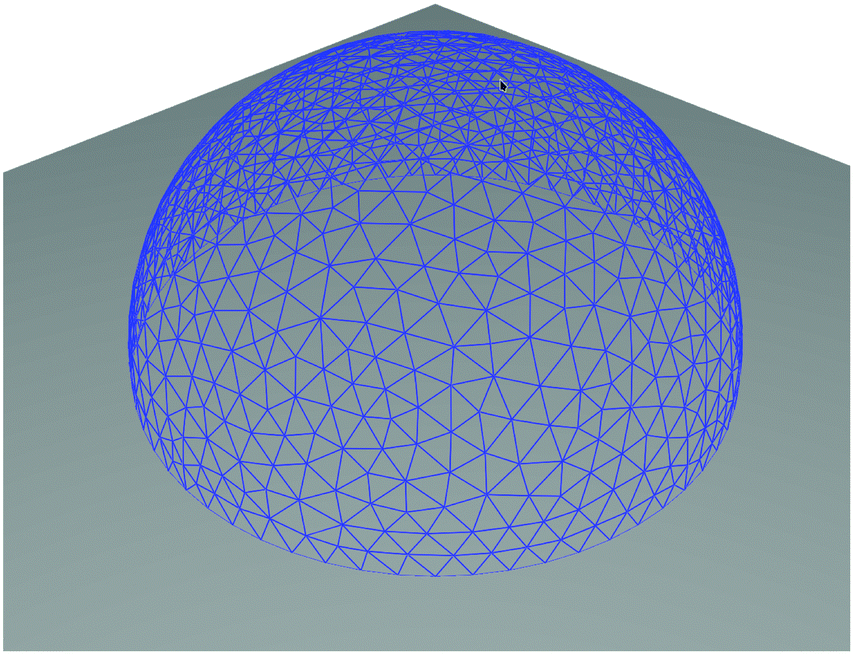 | ||
| Fig. 1 Rendering of a droplet sitting on a substrate (grey surface). The blue mesh indicates its free surface. | ||
2.1 Boundary integral equation for Stokes flow
The boundary element method (BEM) approximates solutions to linear partial differential equations (PDEs) based on their Green's functions.23,25 For droplets moving on substrates we need to study Stokes flow in incompressible fluids, which obeys two linear PDEs for velocity v and pressure p,26| μ∇2v(r) = ∇p(r) and ∇·v(r) = 0, | (1) |
![[Doublestruck R]](https://www.rsc.org/images/entities/char_e175.gif) 3 is the Oseen tensor
3 is the Oseen tensor | (2) |
 | (3) |
3 with boundary ∂D and outward normal described by unit vector n, the flow field fulfills the following integral equation:23,25,26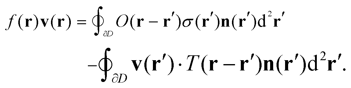 | (4) |
 | (5) |
The Stokes flow problem is only fully determined with boundary conditions. The droplet boundary consists of two parts, one interface with a solid substrate and a second with a gas phase. This means each part has its own boundary condition. At the interface with the substrate there is a Robin boundary condition (for fluids called the Navier condition), μv + λσn = 0, with a slip length λ,34 which connects tangential velocity and tangential stress, while the normal component of v is zero. A typical value for the slip length is λ ≈ 1 nm35 much smaller than the droplet dimension. At the interface towards the gas phase we assume zero viscosity of the gas phase so that the tangential stress is zero. There remains a Neumann boundary condition, n·σn = −2γκ, which locally relates the normal stress component n·σn to the mean curvature κ, where γ is the local surface tension.36 In hydrostatics the stress tensor σ is just −pI and one recovers the expression for the Laplace pressure. However, in our case in the presence of flow the stress tensor σ also includes the viscous part and, therefore, the boundary condition also contains normal derivatives of the flow field.
2.2 Cox–Voinov law for the contact line
Droplets in equilibrium minimize the sum of their surface energies from the interfaces towards the gas phase and substrate, respectively, while preserving their volume.35 If wetting is energetically more favorable than a dry substrate, the liquid phase covers the substrate with a thin film. Otherwise, a droplet forms with an energetically optimal ratio of the areas between liquid–gas and liquid–substrate interfaces. On homogeneous and planar substrates, the optimal shape obviously is a spherical cap. The balance of all forces acting on the three-phase contact line determines the contact angle θeq in equilibrium It results in Young's equation, which relates θeq to the surface tensions γij between liquid (l), gas (g), and substrate (s), respectively:γsg = γsl + γlg![[thin space (1/6-em)]](https://www.rsc.org/images/entities/char_2009.gif) cos(θeq). cos(θeq). | (6) |
Here, when we talk about dynamic wettability patterns, we will vary Δγs = γsg − γsl and thereby θeq in time. On substrates with heterogeneous wettability the optimal droplet shape can be much more complicated including complex shapes of the contact line and varying curvature of the liquid–gas interface.31
The dynamics of the contact line and the contact angle are not directly determined within the approach outlined so far. Because the droplet surface is not smooth at the contact line, it is not clear which boundary condition to use here. For the Neumann boundary condition towards the gas phase the mean curvature κ diverges, while the Navier condition at the substrate does not contain any surface tension necessary to obtain Young's eqn (6) in equilibrium. Therefore, the contact line dynamics has to be determined by an additional relation, which translates the fluid motion in the microscopic contact line region to the macroscopic scale. Several such relations for dynamic wetting exist.35,37–41 The most well-known among them is the Cox–Voinov law40,41 derived from hydrodynamic considerations:
 | (7) |
The velocity vcontact determines the component of the fluid velocity perpendicular to the contact line and in the plane of the substrate. We evaluate θdyn using the surface normal n and the substrate normal ez at the contact line:
| cosθdyn = n(t)·ez. | (8) |
The resulting velocity vcontact of eqn (7) is included in the discretized BEM problem as a boundary condition by introducing a corresponding stress at the contact line as an additional unknown. Furthermore, in the direction of the substrate normal we prescribe a vanishing velocity and along the tangent of the contact line we set the stress to zero. Together, these three conditions fully determine fluid velocity and stress along the contact line.§
On a light-switchable substrate the light patterns affect the surface tension difference Δγs = γsg − γsl in eqn (6). Therefore, as mentioned already, we will treat Δγs as a heterogeneous and dynamic quantity, which locally determines θeq and, thereby, deforms the droplet.
2.3 Discretization
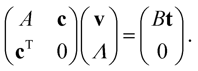
We discretize eqn (4) using a triangular mesh to cover all droplet surfaces (solid–liquid and vapour–liquid). From the triangular mesh we define a dual mesh in which each vertex at position r(i) is surrounded by a compact polygonal region Ci = C(r(i)) (Fig. 2). Together, all the regions Ci cover the entire surface. For a sufficiently fine and well-adapted mesh, field variables are approximately constant on each Ci and integrals can thus be evaluated piece-wisely. As a result, eqn (4) becomes a system of linear equations of the form: | (9) |
 | (10) |
 | (11) |
| Av = Bt. | (12) |
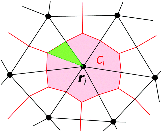 | ||
| Fig. 2 Schematic of triangular mesh (black) in the neighborhood of vertex r(i) and its associated polygonal region Ci (red). The region Ci is defined by and subdivided into triangles, one of which is indicated in green. The three corners of the triangles are the central vertex r(i), the point halfway toward a neighboring vertex r(j), and the centroid (barycenter) of one of the black mesh triangles. | ||
To perform the integrations in eqn (10) and (11), we subdivide the polygonal region Ci into triangles (Fig. 2) and numerically integrate over each triangle using a Gaussian quadrature stencil with 9 points for nonsingular integrands and with 400 points for singular integrands (i.e. when i = j in eqn (10) and (11)).23,28 Note that we never evaluate the integrand at the vertex r(i), where the tensors O or T have integrable singularities, but always choose points inside the triangles for performing the Gaussian quadrature, which is sufficient.
To solve eqn (12), we first apply the boundary conditions introduced above to remove one of the variables at the vertex, either velocity or surface force. Specifically, at the interface towards the gas phase the tangential component of the surface force is zero while we replace the normal component by the Laplace pressure −2γκ. To calculate the principal curvatures at each vertex, we use the discrete Laplace–Beltrami operator described in method C of the review of Guckenberger et al.44 and the normal vector n(i) follows by taking the sum of the normal vectors of all neighboring triangles and normalizing it. At the interface with the solid substrate we set the normal velocity component to zero and eliminate the tangential component of the surface force by the Robin boundary condition. Finally, at the contact line the velocity component normal to the substrate is zero. The in-plane velocity component normal to the contact line obtains the value prescribed by the Cox–Voinov law, and the tangential component of the surface force is zero. We then collect all the remaining unknown variables on the left-hand side and all the known quantities on the right-hand side and solve the resulting system of linear equations by inversion of the coefficient matrix. Finally, the missing velocity and surface-force variables are calculated from the boundary conditions. In total, solving the linear problem of eqn (12) yields approximations for v and σn anywhere on the droplet surface. Once these quantities are known, v(r) can be calculated anywhere within the droplet by numerical integration from eqn (4).
2.4 Time evolution
In the discretized version the dynamics of the free droplet surface is specified by the velocity of each vertex with position vector ri. Concretely, the vertex moves with the local normal component of the fluid velocity and an artificial tangential component w(i)t, which is due to mesh optimization and introduced rigorously in Section 2.6,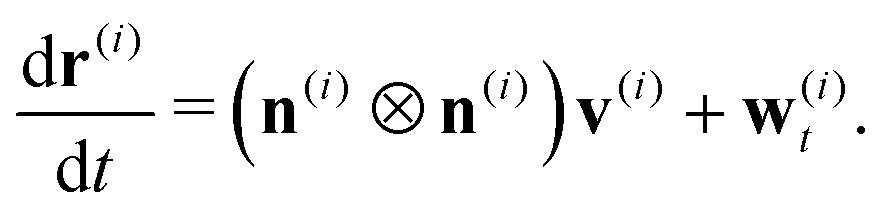 | (13) |
Note that time appears only through eqn (13) in our problem because Stokes flow adapts instantaneously to the droplet's shape. Numerically, the dynamics of each r(i) is calculated using a state-of-the-art Runge–Kutta algorithm45 once the velocity vectors v(i) are calculated with the BEM as described above.
We refine the numerical setting described so far with two additional techniques described in Sections 2.5 and 2.6: a volume constraint and a mesh optimization method.
2.5 Volume constraint
We follow a method first suggested by Alinovi et al.46 to preserve the volume V of the droplet during motion through a side condition for the velocity vectors of the droplet surface. Since volume conservation can be formulated by the chain rule, we obtain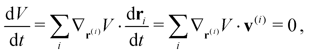 | (14) |
 | (15) |
2.6 Mesh optimization
During the simulation we optimize the mesh representing the droplet meaning we avoid acute-angled triangles and keep the triangle areas uniform across the whole droplet surface. This guarantees that discretization errors remain minimal. According to Zinchenko et al.,27 a mesh fitness is introduced that is maximized for equilateral triangles. It is a function of all the edge lengths of the triangles and their areas. Thus, improving the mesh fitness w.r.t. the triangle shape minimizes discretization errors.Following Zinchenko et al.,27 we apply two measures at different phases of time integration. First, when calculating the r.h.s. of eqn (13), we choose the tangential velocity of each vertex on the free droplet surface including vertices on the contact line such that the rate of change of the overall mesh fitness is minimal.|| We then move all the vertices on the free droplet surface by one Runge–Kutta time step. Note that the normal velocity, which affects droplet shape and motion, remains unchanged. Second, as a next step we check the fitness of the mesh facing the substrate and if the maximum edge lengths exceeds 150% of the minimal edge length, the positions of all substrate vertices (without the ones on the contact line) are adjusted by tangential displacements.**
Since this technique is completely derived from literature and by its very nature must not affect the dynamics of the droplet, we do not reproduce the algorithm in detail here. In Appendix A, Fig. 11 we display mesh fitness over time for a benchmark case to show the effectiveness of the implemented method.
2.7 Nondimensionalization and material parameters
We are able to nondimensionalize our continuum equations by introducing a characteristic length scale R0, a time scale τ, and a force scale fc. Using these three parameters, we will then rewrite all quantities ai as dimensionless quantities ãi. For R0 we choose the radius of the initial circular base area of the droplet. Furthermore, we remove dynamic and kinematic viscosities from our equations, which then implies the characteristic time and force scales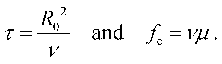 | (16) |
 , slip length
 ![[small lambda, Greek, tilde]](https://www.rsc.org/images/entities/i_char_e0df.gif) = λ/R0, stress tensor components
= λ/R0, stress tensor components ![[small sigma, Greek, tilde]](https://www.rsc.org/images/entities/i_char_e10d.gif) ij = σijR02/fc, and surface tensions
ij = σijR02/fc, and surface tensions ![[small gamma, Greek, tilde]](https://www.rsc.org/images/entities/i_char_e0dd.gif) ij = γijR0/fc. Since the reduced time and coordinates are
ij = γijR0/fc. Since the reduced time and coordinates are ![[t with combining tilde]](https://www.rsc.org/images/entities/i_char_0074_0303.gif) = t/τ and
= t/τ and ![[x with combining tilde]](https://www.rsc.org/images/entities/i_char_0078_0303.gif) = x/R0, the respective reduced derivatives become
= x/R0, the respective reduced derivatives become  and
and  .
.
In ref. 42 de Ruijter et al. considered the relaxation of a droplet on a uniform substrate towards its equilibrium shape assuming that the droplet is always a spherical cap (spherical-cap model). Then, the constant volume V or its reduced value Ṽ is always strictly related to the momentary contact angle. In particular, with the initial contact angle θ0 we have
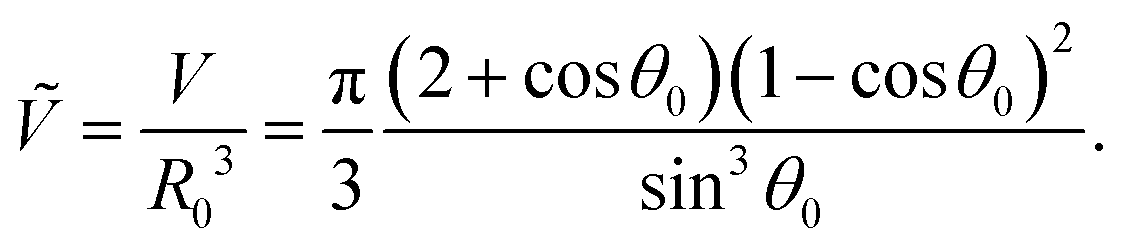 | (17) |
 | (18) |
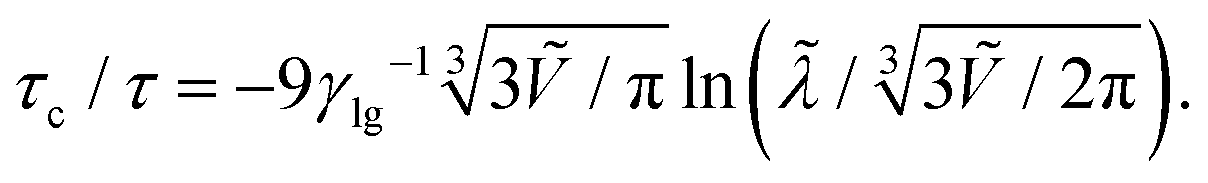
In Table 1 we collect the material parameters and their dimensionless counterparts for a 90% glycerine/10% water mixture for various length values R0 and use them in the following.
, dimensionless slip length , Cox–Voinov-coefficient ln(h/λ), and characteristic time τc for θ = 90°
| # | Material | μ [mPa s] | ν [mm2 s−1] | γ [mN m−1] | λ [nm] | R 0 [μm] | τ [μs] | f c [μN] |
|
|
ln(h/λ) | τ c/τ |
|---|---|---|---|---|---|---|---|---|---|---|---|---|
| a For glycerin, de Ruijter et al.42 fitted θdyn(t) as a solution of eqn (19) to their experimental data and observed the value 44 for ln(h/λ). They interpret this large value as the result of “an additional source of energy dissipation within the three-phase zone”.42 | ||||||||||||
| 1 | 90% glycerol | 209 | 169 | 65.3 | 1 | 100 | 59 | 35 | 0.19 | 10−5 | 44a | 2084 |
| 2 | 90% glycerol | 209 | 169 | 65.3 | 1 | 1500 | 13300 |
35 | 2.8 | 0.67 × 10⁻⁶ | 44a | 141 |
3 Validation: switching a homogeneous substrate
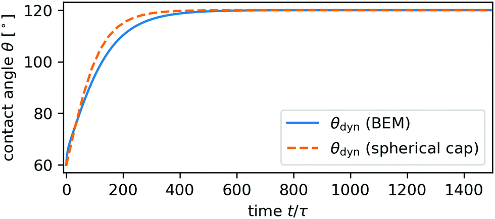
We apply our method to a simple case to validate its performance. The simplest applicable test case is the relaxation of a sessile droplet on a homogeneous substrate that switches from one wettability to another (see Movie M01 in the ESI†). Thus the equilibrium contact angle is switched at a specific time and we observe how the droplet relaxes towards the new equilibrium contact angle. Note that our method includes a valid model for the motion of the contact line because we impose the Cox–Voinov law explicitly. However, the motion of the contact line is coupled to the motion of the free surface and the fluid inside the droplet.In the following we illustrate the overall dynamics of the droplet at a specific system. We rely on experimental data published by de Ruijter et al.42 who observed the spreading of ca. 5–10 mm3 of a 90% glycerol/10% water mixture on PET. All material properties and parameters are collected in Table 1, row 2.
As already explained in Section 2.7 de Ruijter et al. modeled the relaxation of the droplet using the spherical-cap model and used the Cox–Voinov law to completely describe the droplet dynamics by the dynamic contact angle θdyn. It obeys the following differential equation:
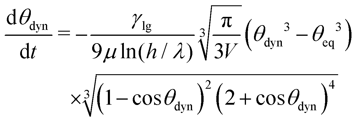 | (19) |
In Fig. 3 we present results for the relaxing glycerin droplet using the material parameters of row 2 in Table 1. We compare our results for the contact angle from the BEM to numerical solutions of eqn (19) in Fig. 3(a). We find qualitative agreement between both approaches. However, the observable deviations of the two curves, the BEM shows a slower relaxation in the contact angle, reveals that the fluid flow included in our method slows the relaxation further down. Our simulated dynamics also matches the experimental results in both the shape of the relaxation curve of the contact angle and relaxation time, as the experimental points in Fig. 3(a) show. We achieve this despite several uncertainties: We know neither the exact initial shape of the droplet in the experiments of de Ruijter et al. nor the exact volume of liquid they used. We also note during our simulations fluctuations in the droplet volume do not exceed 0.15% of the initial volume, while the droplet base radius and height, displayed in Fig. 3(b), change by over 20% of their initial values. This clearly demonstrates the robustness of our implementation. Finally, in Fig. 4 we display the stream lines of the fluid at t = 7τ, along which material is transported from the top to the sides of the droplet as it spreads.
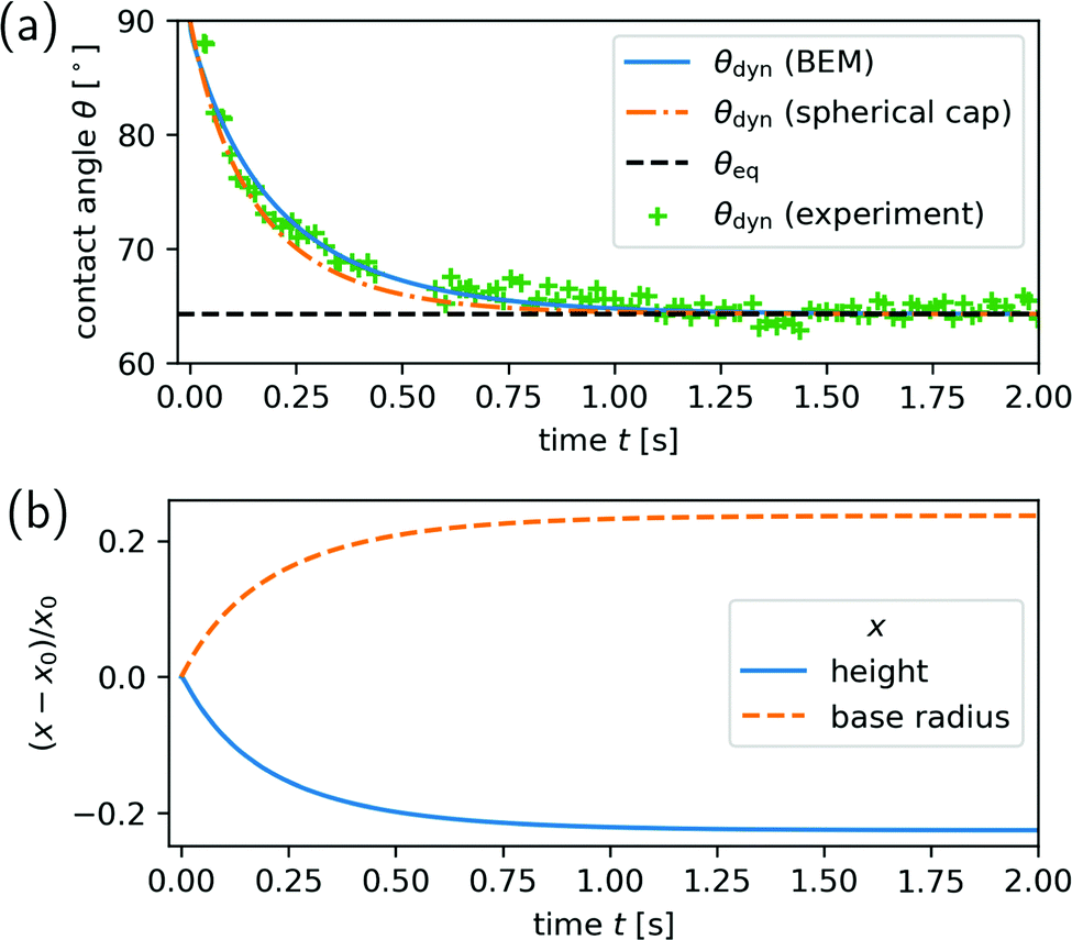 | ||
| Fig. 3 Relaxation of a 90% glycerol droplet after the wettability of the substrate is switched from an equilibrium contact angle of 90° to θeq = 65° at time t = 0: (a) dynamics of the contact angle θdyn plotted versus time. Solid blue line shows the result from the BEM and dashed-dotted orange line from the spherical-cap model. The dashed black line shows the final equilibrium contact angle. The symbols refer to experimental data points reproduced from Fig. 2(a) in ref. 42. (b) Deformation of the droplet as a function of time either characterized by droplet height (solid blue line) or radius of the base area (dashed orange line). The change relative to the respective initial values x0 are shown. Both curves are calculated with the BEM. | ||
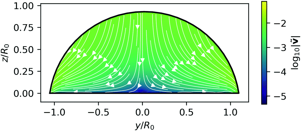 | ||
| Fig. 4 Computed stream lines (white solid) in the central cross section of the 90% glycerol droplet at t = 7τ. Its outline is the solid black line and background color indicates speed. The streamlines follow within the BEM. | ||
We also studied a number of wettability switches on homogeneous substrates to test the technical limitations of our mesh stabilization. Specifically, we were able to realize changes in contact angle of ±15° when starting from 60° and ±30° when starting from 90°. Notably, the latter case means that our method is able to cross into regions where droplets overhang their base area without any special modifications to treat this case. For example, in Fig. 5 we demonstrate the relaxation of the contact angle from θdyn = 60° to θeq = 120°. (A corresponding animation is included as Movie M01 in the ESI†.) A clear deviation from the spherical-cap model is visible.
 | ||
| Fig. 5 Relaxation of the contact angle from 60° to 120° of a 90% glycerol/10% water droplet with R0 = 100 μm on a homogeneous substrate. | ||
4 Surfing on a wettability step profile with feedback
A droplet placed on a substrate with a gradient in wettability will move in the direction of increasing wettability meaning smaller contact angle. In the following two sections we consider a smooth step profile in wettability (cf.Fig. 6). In this Section 4 we use a feedback loop to move the step with the droplet so that the distance between wettability step and the droplet's center of mass stays constant. Thus, the droplet quasi “surfs” on the wettability step (see Movie M02 in ESI†). Then, in Section 5 we will move the wettability step with fixed speed and monitor the motion of the droplet. We will demonstrate that the feedback-regulated droplet motion agrees with the moving-droplet state found for a fixed step speed.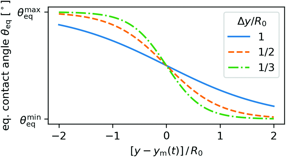 | ||
| Fig. 6 Three examples for a step profile in wettability quantified according to eqn (20) by the equilibrium contact angle. ym is the center of the wettability step with maximal gradient and Δy its width. | ||
4.1 Setup
In our approach we quantify the wettability of the substrate by the local equilibrium contact angle. To realize a step profile in wettability, θeq(y,t) (displayed in Fig. 6), we use the logistic step function and write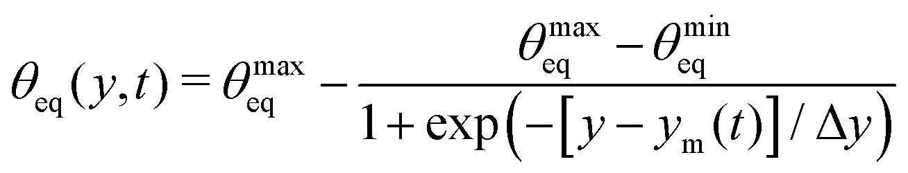 | (20) |
Here, all droplets are simulated using the material properties set out in row 1 of Table 1 which describes a 90% glycerol/10% water mixture with R0 = 100 μm.
4.2 Flow field
Regardless of the specific values for each parameter for the wettability step, the droplet eventually settles into a steady state with constant shape and constant flow field. The moving droplet never adjusts to the local equilibrium angles exactly. Rather a difference remains between θdyn and θeq, which drives the droplet and determines its steady-state speed | (21) |
As a representative example, in Fig. 7 we display the internal flow field of a droplet surfing on a wettability step characterized by θmineq = 90°, θmaxeq = 120°, and Δy = 1/3 at an offset s = 0, i.e., directly on the steepest location. The flow field forms one single vortex filling the droplet in the plane parallel to its direction of motion and two vortices in the plane perpendicular to this direction. The fluid is transported predominantly along the free surface and so, in effect, it rolls on the substrate as the droplet moves forward.
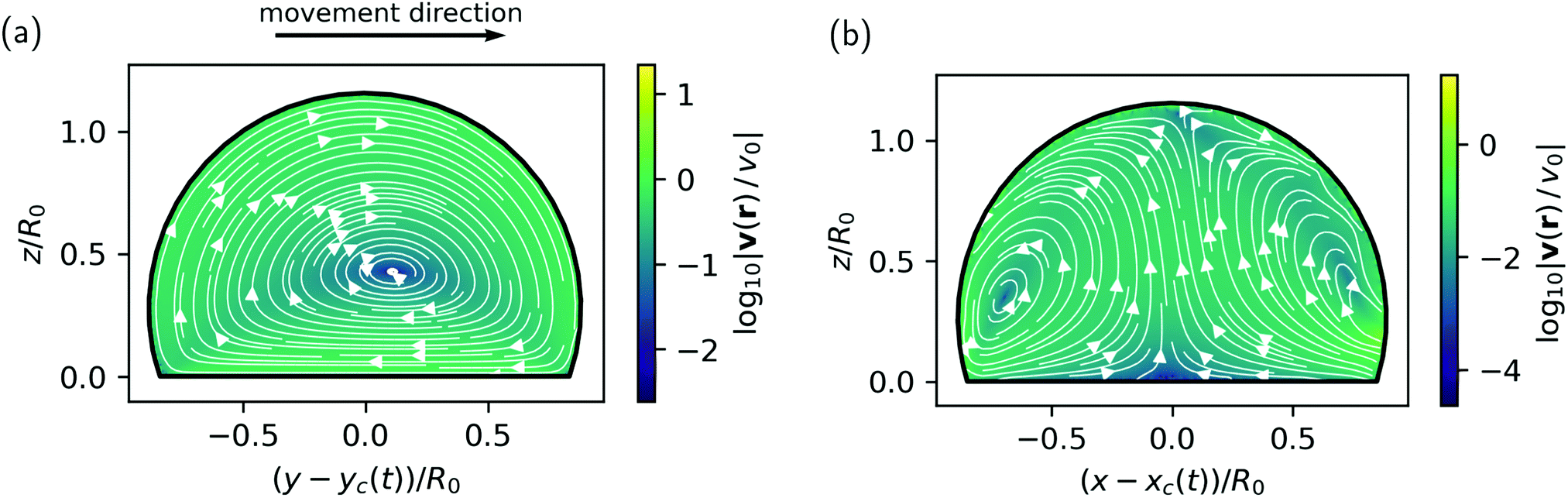 | ||
| Fig. 7 Flow field in the interior of the droplet (a) in the comoving reference frame of the droplet moving with speed v0, and (b) in a cross-sectional plane perpendicular to the direction of motion for a 90% glycerol/10% water droplet with R0 = 100 μm “surfing” with θmineq = 90°, θmaxeq = 120°, Δy = 1/3, and s = 0. An animation of point-like tracer particles corresponding to (a) is contained in the ESI† as Movie M05. | ||
4.3 Speed
The steady-state droplet speed v0 depends on the various parameters of the wettability profile. In Fig. 8(a) we plot the droplet speed versus the offset s for several parameter sets structured by (i) the limiting equilibrium contact angles on both sides of the wettability step and (ii) the step width Δy.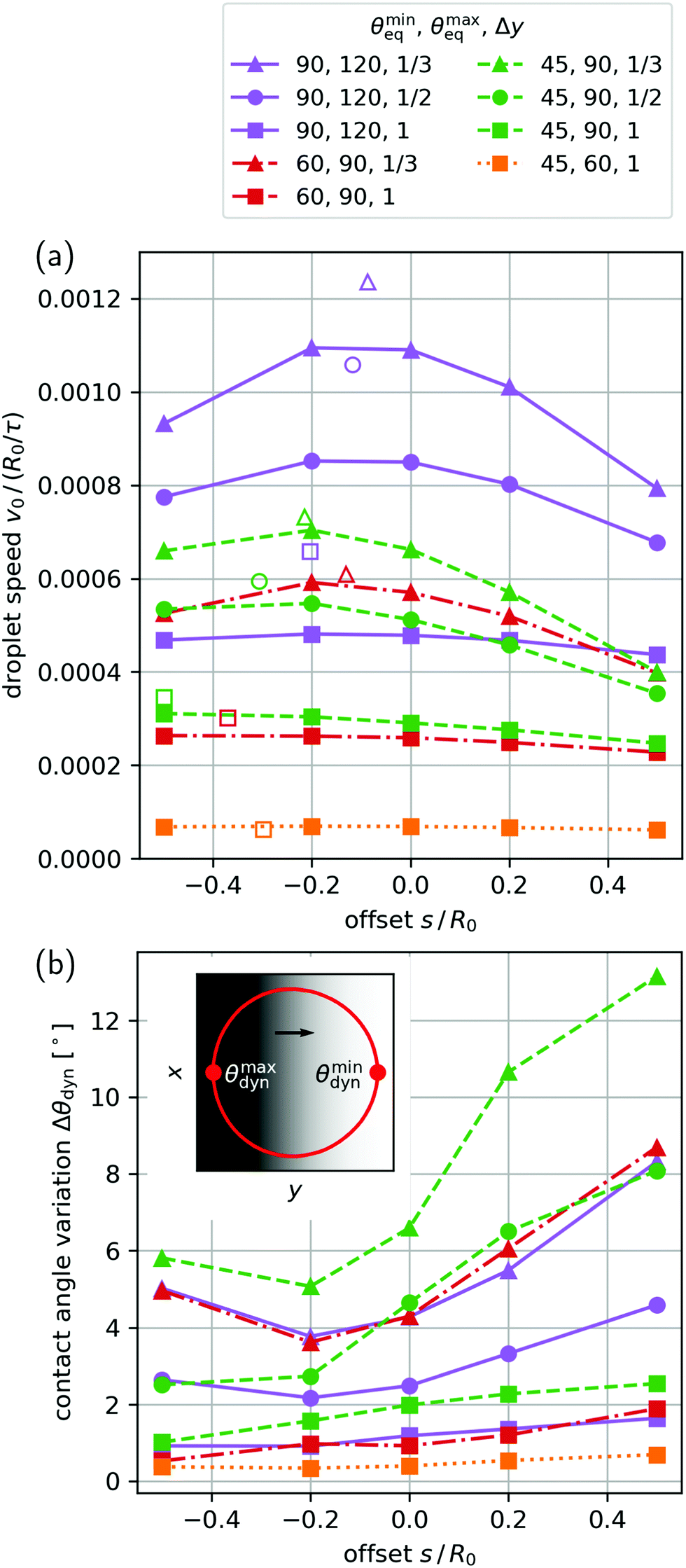 | ||
| Fig. 8 Steady-state (a) speed v0 and (b) maximal contact-angle difference Δθdyn plotted versus offset s for various feedback-driven droplets of a 90% glycerol/10% water mixture in response to wettability step profiles characterized by different parameter sets (see legend). Lines between symbols are added to guide the eye. The open symbols in (a) show estimates for the maxima of the curves using the spherical-cap model as outlined in Appendix C. Inset in (b): Example for a contact line (red) surfing on a wettability step (background shading) with markers for the locations of θmindyn and θmaxdyn (circles). | ||
First of all, we observe that v0 increases overall with decreasing Δy which is consistent with the expectation that steepness of the wettability step drives the droplet forward. Furthermore, as Δy decreases for the same combinations of contact angles, an optimal offset s becomes prominent close to s = −0.2R0 (circle and triangle symbols in Fig. 8(a)), meaning the droplet lags behind the step and is pushed forward. Since the wettability gradient is largest at s = 0, we conclude that the steepness of the wettability step does not solely determine droplet speed. Rather, there is a competing influence from the fact that the equilibrium contact angles θmaxeq and θmineq contribute nonlinearly to droplet speed via the contact line. According to the Cox–Voinov law the speed of the contact line depends on the difference of the cubes of θdyn and θeq. Thus, v0 increases with θeq even when the difference θdyn − θeq remains the same. As a result, the droplet speed increases for larger θeq, which the droplet encounters if it lags behind at s < 0.
This is nicely visible in Fig. 8(a), when we compare the 60° to −90° combination in equilibrium contact angles (red symbols/dash-dotted lines) to the 90° to −120° combination (purple symbols/full line). Even though the difference between the limiting angles is 30° in both cases, the droplet speed is larger for the larger equilibrium contact angles.
We estimate the magnitude of this effect in Appendix C, where we extend the spherical-cap model to describe a surfing droplet. We are able to derive a relation, which shows how the maximum surfing speed vmax depends on the wettability contrast determined by θmineq and θmaxeq:
 | (22) |
4.4 Deformation
Since the droplets are placed on a non-uniform wettability pattern, their shapes adapt and become asymmetric. There is a competition between the Laplace pressure depending on the local curvature of the free surface, which drives the droplet toward a uniform curvature, and the forces acting on the contact line, which drive the local contact angle toward its equilibrium value. Therefore, the free surface will deviate from a spherical cap. The result of these competing forces can be observed in the variation of the dynamic contact angle θdyn along the contact line in steady state. To quantify this variation, we plot in Fig. 8(b) the difference of the largest and smallest contact angle, Δθdyn = θmaxdyn − θmindyn, versus the offset s for the different parameter sets. Simply put, a larger difference Δθdyn indicates a more asymmetric droplet shape. Note that θmindyn and θmaxdyn are realized at the front and the back of the droplet w.r.t. to its direction of motion as indicated in the inset of Fig. 8(b), where the equilibrium contact angles are extremal. At these locations the contact line velocity vcontact must equal the droplet speed v0 in steady state. So the difference between the extrema of θdyn and θeq along the contact line determines v0.We observe that Δθdyn is primarily determined by large variations in θeq, which makes sense. For example, the wettability profiles with θmineq = 45° and θmaxeq = 90° [green symbols/dashed lines in Fig. 8(b)] cause larger variations Δθdyn than step profiles with θmineq = 90° and θmaxeq = 120° [purple symbols/solid lines in Fig. 8(b)] for otherwise same parameters.
In addition, for Δy/R0 = 1/3 and 1/2, Δθdyn shows a strong dependence on the offset s. Interestingly, for these cases the droplet asymmetry decreases notably as s approaches the speed optimum s = −0.2R0. Apparently, a more symmetric droplet has larger differences between θdyn and θeq along its contact line and therefore achieves higher speeds v0. In Appendix C we show, using the spherical-cap model, that droplets with symmetric shape move faster than the asymmetric droplets observed here. A comparison of the optimal speed values estimated from the model and the simulation results [both displayed in Fig. 8(a)] reveals the following. While the model overestimates droplet speed, it reproduces the optimal offset, i.e., the fact that the fastest droplets lag behind.†† Because the model only considers perfectly symmetric droplets, the higher speed for lagging droplets can be attributed to the nonlinear dependence of the Cox–Voinov law on θdyn and θeq as explained at the end of Section 4.3.
In summary, we observe droplets settle into a rolling motion when they are a placed on a wettability step profile with a constant offset to the location of steepest wettability gradient. Their limiting speed increases with the steepness of the gradient. For large steepness there is an optimal offset so that the droplets are pushed forward by regions of lower overall wettability. Their shapes become more asymmetric in response to steeper gradients, while the optimal offset for speed is correlated with a more symmetric shape.
5 Wettability step profile with constant driving
5.1 Setup
As an alternative to the feedback method described above, we study the simpler setup where the wettability step of eqn (20) moves with constant speed. Here, two scenarios are possible: if the droplet can keep up with the moving wettability profile, it will surf on the pattern, otherwise it will fall behind, stop moving, and eventually adapt its shape to the lower wettability of the substrate.To gain insight into these scenarios, we re-examine one particular pattern from the previous part: a wettability step with θmineq = 90° and θmaxeq = 120°, and Δy = 1/3. We place a glycerol droplet with parameters according to row 1 of Table 1 well before the step and, unlike before, let the step approach the droplet with a constant speed vs independent of the position of the droplet.
5.2 Long-time dynamics
We first position the droplet at t = 0 with an initial lead s0 = 2R0 before the steepest point of the step, which means the droplet is on the more wettable side of the step. This gives the droplet some time to adapt to a surfing shape under the influence of the approaching step. We then observe how the droplet lead,| s(t) = yc(t) − vst + s0, | (23) |
In Fig. 9 we display trajectories leading to either droplets surfing on the wettability step or droplets that cannot follow. Above a step speed of roughly vs = 1.1 × 10⁻³R0/τ droplets cannot keep up with the step meaning their droplet lead tends to minus infinity. Below, droplets match the step speed and surf, meaning their droplet lead approaches a constant value. In both scenarios the droplets deform in response to the wettability step (cmp. insets in Fig. 9). However, in the first case they eventually relax into an equilibrium shape, i.e., a spherical cap with an increased contact angle, while in the second case they take on an asymmetric surfing shape. At the transition between both scenarios the droplets achieve their maximum surfing speed. In Appendix C we estimate its value using the spherical-cap model and show its dependence on the wettability contrast for several minimum contact angles in Fig. 12. In our simulations, the transition occurs close to the maximum droplet speed of 1.1 × 10⁻³R0/τ, which we observed using the feedback mechanism in Section 4.3, Fig. 8(a). Furthermore, we note that the droplet lead of 0.24R0 observed for vs = 10−3R0/τ is close to the lead 0.2R0, which occurred for a similar speed of v0 = 1.01 × 10⁻³R0/τ in Section 4.3 [purple triangles in Fig. 8(a)].
 | ||
| Fig. 9 Droplet lead s with initial value s0 = 2R0 plotted versus step displacement vst. The wettability step is characterized by θmineq = 90°, θmaxeq = 120°, and Δy = 1/3 and for the droplet glycerol parameters (row 1 in Table 1) are taken. Solid lines indicate trajectories for various vs as indicated in the legend. Insets: Snapshots of droplet shapes shown from above with droplet surface (light blue), contact line (solid red), and wettability profile (background shading). The arrows point to the moments at which the snapshots are taken (see also Movies M06 and M07 in ESI†). | ||
So far, we can draw two conclusions from our investigations in comparison to the feedback studies of the previous section. First, for a given step speed a droplet sitting ahead of the approaching wettability step assumes the offset s given in the upper curve of Fig. 8(a) by the branch to the right of the maximum. Second, droplets cannot follow wettability steps with larger speeds.
5.3 Preferred surfing state
How does the final surfing state of the droplet depend on the initial droplet lead s0? To answer this question, we placed a droplet with initially spherical cap shape and initial contact angle θdyn = 90° at different positions relative to the wettability step, which moved with different velocities. The result is presented in the state diagram s0vs. vs of Fig. 10. The black solid-dashed line indicates the result from the feedback analysis in Fig. 8(a). The yellow triangles mean that the droplet lead decreases. For vs ≤ 1.1R0/τ, when the lead reaches the upper branch of the black curve, the droplet is taken along by the step and moves with constant speed. For vs > 1.1R0/τ the droplet cannot follow the wettability step and is left behind (see Movies M03 and M07 in ESI†). The blue triangles inside the black curve indicate droplets that initially move faster than the wettability step. The droplet lead s increases until it hits again the solid black line and the droplet again moves with constant speed vs (see Movies M04 and M06 in ESI†). | ||
| Fig. 10 Moving direction of the droplet plotted in a diagram versus initial lead s0 and step speed vs. Blue and yellow triangles indicate decreasing or increasing droplet lead, respectively. The black solid-dashed curve corresponds to the steady-state motion from the feedback study in Section 4 [cf. the purple triangles in the upper curve of Fig. 8(a)]. As the blue and yellow triangles show, the solid black curve also gives the final offset s∞ of a droplet surfing steadily on a moving wettability step. Same parameters as in Fig. 9 are used. | ||
Therefore, the solid black line in Fig. 10 taken from our feedback analysis gives exactly the resulting lead s∞ of a droplet constantly moving with the step profile when starting with an initial lead above the dashed black line. It also indicates the maximum step speed for dragging a droplet along. From the perspective of non-linear dynamics the solid line is a stable branch indicating that the droplet will mostly move in front of the wettability step (s∞ > 0). In contrast, the positions given by the dashed line are unstable. This behavior is reminiscent of a saddle-node bifurcation near vs ≈ 1.1R0/τ. Our results also show that for droplets on wettability steps feedback has a stabilizing effect on an otherwise unstable state (see, e.g., ref. 47).
The (in)stability of either branch is intuitively explained by the steepness and local curvature of the sigmoid curve, which we use for the wettability profile (see Fig. 6): By definition, a leading droplet is on the convex part of the sigmoid which means, as it falls behind it is exposed to an increasing gradient which speeds it up again. Conversely, a lagging droplet is on the concave part of the sigmoid and as it falls behind it is exposed to a decreasing gradient which slows it down further. Only close to the turning point also lagging positions are stable. We explain this by the fact that the droplet is an extended object. The unstable and stable positions meet at the bifurcation point, which is near the steepest part of the sigmoid. There, the droplet is exposed to the largest possible gradient and therefore achieves its maximum speed.
6 Conclusions
In this article we have applied the boundary element method and developed a numerical scheme to simulate droplets on substrates with switchable and non-uniform wettability realized, for example, by light-switchable surfaces. A strong emphasis was put on developing a stable grid on the droplet surface. We are able to simulate droplets on the whole range of possible contact angles and, in particular, investigated speed and deformation of droplets under the influence of moving wettability steps. A crucial ingredient for simulating the dynamics of droplets is the Cox–Voinov law, which governs the motion of the three-phase contact line. In addition, using the boundary element method allows us to calculate flow fields inside the droplet and not just on its surface and thereby provides a further understanding of the droplet motion.We first applied our method to sessile droplets and exposed them to a spatially uniform but instantaneous change in wettability. We carefully compared our findings to experimental results from ref. 42 and found quantitative agreement. The spherical-cap model, where the dynamics is governed by the dynamics of the contact line via the Cox–Voinov law, shows small but noticeable differences.
We then applied our numerical scheme to droplets surfing on moving wettability steps. First, using a feedback loop we kept the center of the wettability step at a constant distance or offset from the droplet center. For a range of offsets and step widths, this gives rise to droplets surfing at constant speed on the wettability step into the direction of higher wettability. Inside the droplet a single vortex forms such that the droplet rolls on the substrate. For shallow wettability steps the resulting droplet speed hardly depends on the droplet offset in the range investigated. However, for steeper steps the speed develops a maximum at offsets behind the steepest point of the step so that the droplet experiences regions of lower overall wettability. Additionally, while droplets surfing on steep steps are less symmetric compared to more shallow steps, droplets surfing with the maximum speed are more symmetric compared to slower droplets on the same wettability profile.
In a second study we moved the wettability step at a constant speed with various initial offsets between the step and droplet center. Beyond the maximal droplet speed from the feedback study, steady surfing is not possible. The droplet cannot follow the wettability step and is left behind. Below the maximal surfing speed, droplets always settle to the same offset as observed in the feedback study. However, only the leading positions where the droplet is pushed forward are stable, while the lagging positions are unstable in the absence of feedback. We explain this by the curvature of the smooth wettability step: In the leading position the convex variation of the wettability step generates an effective restoring force when the droplet is left behind, while in the lagging position the concave variation cannot stabilize the surfing droplet against small displacements away from the step center.
Our findings demonstrate how a dynamic wettability profile, for example, controlled by structured light can be used to continuously drive droplets forward. We have investigated here the important parameters to optimize the speed of droplets w.r.t. the shape of the wettability profile and its driving speed. Because a single wettability step can be set up to move droplets in any direction, in principle, we provide here a tool to steer droplets along arbitrary paths and with variable speed on a light-switchable substrate. In the future, we plan to investigate droplet dynamics in more complex spatio-temporal wettability patterns motivated by the possibilities of structured light.11
Conflicts of interest
There are no conflicts to declare.A Mesh degradation
Over the course of a simulation, mesh fitness M (see ref. 27 for definition) degrades due to physically necessary changes in the mesh shape. In Fig. 11 we give an example of mesh degradation during the initial relaxation of a droplet on a uniform substrate presented in Section 3. Notably, M initially decreases roughly linearly while the droplet changes shape, as visible in Fig. 3. However, M decreases further thereafter which implies that, even in the absence of further deformations, numerical error still compounds. Small numerical errors have a compounding effect on M because M is a nonlinear function of vertex positions, and therefore displacements of similar magnitude have a small effect on the initial (effectively optimal) initial mesh for t < 1 s and a disproportionally larger effect on the already deformed mesh for t > 1 s. | ||
| Fig. 11 The mesh fitness M for a sessile glycerol droplet decreases over time in response to a wettability change at t = 0 s. | ||
B Parameters used for movies in ESI†
All movies visualize simulations with material parameters from row 1 of Table 1. Movie M01 (ESI†) corresponds to the last example provided in Section 3 and Fig. 5, which means it shows an instantaneous change in uniform wettability from θeq = 60° to 120°. Movie M02 (ESI†) corresponds to the purple triangle at offset −0.2R0 in Fig. 8(a). Movie M03 (ESI†) shows a droplet driven by a wettability step from 90° to 120° with steepness Δy = 1/3, step speed of vs = 2 × 10⁻³R0/τ, and an initial lead of s0 = 2R0. Movie M07 (ESI†) shows the same droplet from directly above with its contact line drawn in red. Movie M04 (ESI†) corresponds to the same parameters, except vs = 1 × 10⁻³R0/τ. Movie M06 (ESI†) shows another surfing droplet with the same parameters, except vs = 1.1 × 10⁻³R0/τ, from above with its contact line drawn in red. Movie M05 (ESI†) corresponds to the parameters given in Fig. 7. Note that the movies each run at different speeds.C Speed estimate for spherical-cap droplets surfing on a wettability step
In Section 4.3 we observe that the droplets which move fastest in the feedback setup tend to have the most symmetric shape when compared to slower droplets on the same wettability profile. The limit of droplet axisymmetry are spherical caps. To distinguish the contribution of shape asymmetry from other factors, we consider here the simplified case of droplets that are geometrically constrained to the shape of a spherical cap.Based on this constraint, we use eqn (7) (the Cox–Voinov law) to estimate the speed of a droplet surfing on a given wettability profile. For steady droplet motion the velocities of the contact line at the front and the back of the droplet must match exactly. Using the sign convention of the Cox–Voinov law, this means vfrontcontact = −vbackcontact, and together with constant θdyn along the contact line of a spherical-cap droplet, eqn (7) gives
 | (24) |
| θfronteq = θeq(s + R) θbackeq = θeq(s − R). | (25) |
 | (26) |
Note by choosing the fully symmetric spherical-cap droplet, anything we observe here must be due to the properties of the Cox–Voinov law and the wettability profile under consideration.
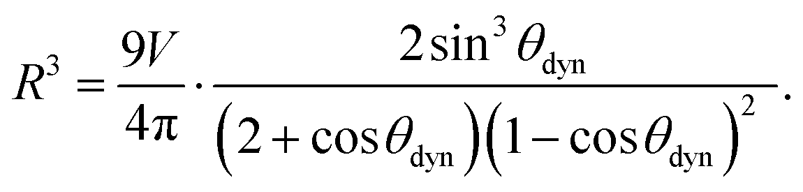
First, we estimate the maximum attainable surfing speed vmax for a wettability contrast Δθeq = θmaxeq − θmineq by considering the limit of R ≫ Δy in eqn (20). In effect, we consider the maximum possible contrast of a given substrate material here, which means we estimate an upper bound on the speed of droplets with finite R. Substituting eqn (24) with θfronteq = θmineq and θbackeq = θmaxeq into eqn (7) for the droplet front gives
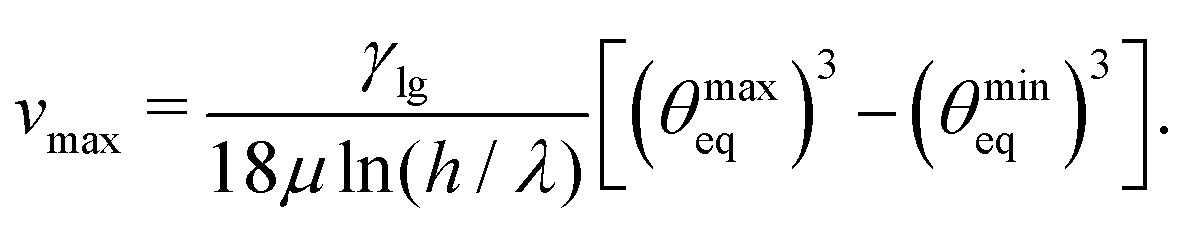 | (27) |
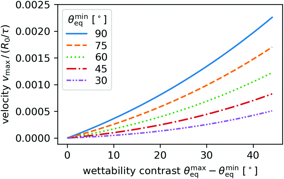 | ||
| Fig. 12 Estimated maximum surfing speed vmax plotted versus contact angle contrast θmaxeq − θmineq for different minimum contact angles θmineq for glycerol parameters (row 1 in Table 1). | ||
Second, we study the effect of the droplet offset s in the wettability step on the estimated surfing speed to develop an understanding for our findings in Fig. 8(a) and 10. Since smaller droplets cannot necessarily extend from the least to the most wettable region of a given wettability step, their optimal surfing position is not a priori clear. We follow the numerical procedure described at the beginning of this section and display surfing speed v versus s in Fig. 13 for the same wettability step profiles as in Fig. 8. The estimated speed values qualitatively match our findings in Fig. 8(a). The droplet speed depends on the minimum and maximum contact angles, and the overall steepness of the step. In particular, for small steepness parameters Δy the pronounced maxima are recovered. Their positions s roughly match the positions observed in Fig. 8, which indicates that the spherical-cap model is well suited to estimate the droplet speed near the maximum. So the spherical-cap model, which we introduced based on the observation that for the maximum surfing speed the asymmetry in the droplet shape is small, provides a good estimate for this maximum. In contrast, the spherical-cap model overestimates the surfing speed compared to our simulations in cases with strong shape asymmetry (cmp. triangles in Fig. 8 and 13). Furthermore, droplet speed is more sensitive to shape asymmetry in cases with large θmineq (cmp. squares in Fig. 8 and 13) which is likely an effect of the nonlinearity illustrated in Fig. 12. Our observations underline that the optimal offset positions for the droplet surfing speed are a consequence of the nonlinear Cox–Voinov law (as noted in Section 4.3) and not of the asymmetry in droplet shape. Thus, the estimate for the droplet speed based on the spherical-cap model provides a useful guide for experiments towards the optimal surfing speed in wettability step profiles.
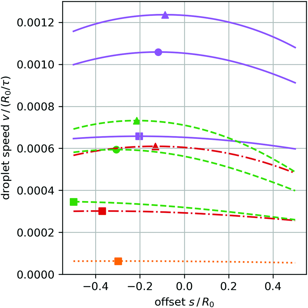 | ||
| Fig. 13 Estimated surfing speed v plotted versus offset s for different wettability step profiles as given in the legend, which is the same as in Fig. 8. The glycerol parameters (row 1 in Table 1) are taken. Markers indicate the maxima on the interval [−0.5R0,0.5R0]. | ||
Acknowledgements
We thank T. Mallouk, D. Peschka, and J. Simmchen for helpful discussions and acknowledge financial support from DFG (German Research Foundation) via Collaborative Research Center 910.References
- M. K. Chaudhury and G. M. Whitesides, Science, 1992, 256, 1539 CrossRef CAS.
- K. Ichimura, S. Oh and M. Nakagawa, Science, 2000, 288, 1624 CrossRef CAS.
- S. Palagi, A. G. Mark, S. Y. Reigh, K. Melde, T. Qiu, H. Zeng, C. Parmeggiani, D. Martella, A. Sanchez-Castillo, N. Kapernaum, F. Giesselmann, D. S. Wiersma, E. Lauga and P. Fischer, Nat. Mater., 2016, 15, 647–653 CrossRef CAS.
- S. N. Varanakkottu, M. Anyfantakis, M. Morel, S. Rudiuk and D. Baigl, Nano Lett., 2016, 16, 644 CrossRef CAS.
- J. Grawitter and H. Stark, Soft Matter, 2018, 14, 1856 RSC.
- K. Seki and M. Tachiya, J. Phys.: Condens. Matter, 2005, 17, S4229 CrossRef CAS.
- E. Chevallier, A. Mamane, H. A. Stone, C. Tribet, F. Lequeux and C. Monteux, Soft Matter, 2011, 7, 7866–7874 RSC.
- D. Baigl, Lab Chip, 2012, 12, 3637 RSC.
- M. Schmitt and H. Stark, Phys. Fluids, 2016, 28, 012106 CrossRef.
- Y. Xiao, S. Zarghami, K. Wagner, P. W. K. C. Gordon, L. F. D. Diamond and D. L. Officer, Adv. Mater., 2018, 30, 1801821 CrossRef.
- H. Rubinsztein-Dunlop, A. Forbes, M. V. Berry, M. R. Dennis, D. L. Andrews, M. Mansuripur, C. Denz, C. Alpmann, P. Banzer, T. Bauer, E. Karimi, L. Marrucci, M. Padgett, M. Ritsch-Marte, N. M. Litchinitser, N. P. Bigelow, C. Rosales-Guzmán, A. Belmonte, J. P. Torres, T. W. Neely, M. Baker, R. Gordon, A. B. Stilgoe, J. Romero, A. G. White, R. Fickler, A. E. Willner, G. Xie, B. McMorran and A. M. Weiner, J. Opt., 2017, 19, 013001 CrossRef.
- F. Mugele, A. Klingner, J. Buehrle, D. Steinhauser and S. Herminghaus, J. Phys.: Condens. Matter, 2005, 17, S559 CrossRef CAS.
- T. M. Squires and S. R. Quake, Rev. Mod. Phys., 2005, 77, 977 CrossRef CAS.
- A. A. Darhuber and S. M. Troian, Annu. Rev. Fluid Mech., 2005, 37, 425 CrossRef.
- O. Kašpar, H. Zhang, V. Tokárová, R. I. Boysen, G. R. Suñé, X. Borrise, F. Perez-Murano, M. T. W. Hearn and D. V. Nicolau, Lab Chip, 2016, 16, 2487 RSC.
- R. Blossey, Nat. Mater., 2003, 2, 301 CrossRef CAS.
- M. Edalatpour, L. Liu, A. Jacobi, K. Eid and A. Sommers, Appl. Energy, 2018, 222, 967 CrossRef.
- Y. Li, Y. Sheng and H. Tsao, Langmuir, 2013, 29, 7802 CrossRef CAS.
- S. Wang, Y. Song and L. Jiang, J. Photochem. Photobiol., C, 2007, 8, 18 CrossRef CAS.
- F. Zhu, S. Tan, M. K. Dhinakaran, J. Cheng and H. Li, Chem. Commun., 2020, 56, 10922 RSC.
- H. S. Lim, J. T. Han, D. Kwak, M. Jin and K. Cho, J. Am. Chem. Soc., 2006, 128, 14458 CrossRef CAS.
- F. Pirani, A. Angelini, F. Frascella, R. Rizzo, S. Ricciardi and E. Descrovi, Sci. Rep., 2016, 6, 31702 CrossRef CAS.
- C. Pozrikidis, Boundary integral and singularity methods for linearized viscous flow, Cambridge University Press, Cambridge, 1992 Search PubMed.
- C. Pozrikidis, J. Comput. Phys., 2001, 169, 250 CrossRef CAS.
- C. Pozrikidis, A practical guide to boundary element methods with software library BEMLIB, CRC Press, Boca Raton/FL, 2002 Search PubMed.
- S. Kim and S. J. Karrila, Microhydrodynamics, Dover Publications, Mineola/NY, 2005 Search PubMed.
- A. Z. Zinchenko and R. H. Davis, J. Fluid Mech., 2013, 725, 611 CrossRef.
- J. T. Katsikadelis, The Boundary Element Method for Engineers and Scientists, Elsevier, 2nd edn, 2016 Search PubMed.
- J. D. McGraw, T. S. Chan, S. Maurer, T. Salez, M. Benzaquen, E. Raphaël, M. Brinkmann and K. Jacobs, Proc. Natl. Acad. Sci. U. S. A., 2016, 113, 1168 CrossRef CAS.
- T. S. Chan, J. D. McGraw, T. Salez, R. Seemann and M. Brinkmann, J. Fluid Mech., 2017, 828, 271 CrossRef CAS.
- K. B. Glasner, J. Comput. Phys., 2005, 207, 529 CrossRef.
- N. Savva, D. Groves and S. Kalliadasis, J. Fluid Mech., 2019, 859, 321 CrossRef CAS.
- C. Gao, L. Wang, Y. Lin, J. Li, Y. Liu, X. Li, S. Feng and Y. Zheng, Adv. Funct. Mater., 2018, 28, 1803072 CrossRef.
- S. J. Bolaños and B. Vernescu, Phys. Fluids, 2017, 29, 057103 CrossRef.
- D. Bonn, J. Eggers, J. Indekeu, J. Meunier and E. Rolley, Rev. Mod. Phys., 2009, 81, 739 CrossRef CAS.
- A. A. Nepomnyashchy, M. G. Velarde and P. Colinet, Interfacial Phenomena and Convection, Chapman & Hall/CRC, New York, 2002 Search PubMed.
- H. B. Eral, D. J. C. M. ’t Mannetje and J. M. Oh, Colloid Polym. Sci., 2013, 291, 247 CrossRef CAS.
- R. Ledesma-Aguilar, A. Hernández-Machado and I. Pagonabarraga, Phys. Rev. Lett., 2013, 110, 264502 CrossRef CAS.
- J. H. Snoeijer and B. Andreotti, Annu. Rev. Fluid Mech., 2013, 45, 269 CrossRef.
- O. V. Voinov, Fluid Dyn., 1976, 11, 714 CrossRef.
- R. G. Cox, J. Fluid Mech., 1986, 168, 169 CrossRef CAS.
- M. J. de Ruijter, J. De Coninck, T. D. Blake, A. Clarke and A. Rankin, Langmuir, 1997, 13, 7293 CrossRef CAS.
- Y. A. Pityuk, O. A. Abramova, N. A. Gumerov and I. S. Akhatov, Math. Models Comput. Simul., 2018, 10, 209 CrossRef.
- A. Guckenberger, M. P. Schraml, P. G. Chen, M. Leonetti and S. Gekle, Comput. Phys. Commun., 2016, 207, 1–23 CrossRef CAS.
- C. Tsitouras, Comput. Math. Appl., 2011, 62, 770 CrossRef.
- E. Alinovi and A. Bottaro, J. Comput. Phys., 2017, 356, 261 CrossRef.
- K. Pyragas, Phys. Lett. A, 1992, 170, 421 CrossRef.
Footnotes |
| † Electronic supplementary information (ESI) available: Their descriptions are collected in Appendix B. See DOI: 10.1039/d0sm02082f |
| ‡ The solid angle is calculated locally by considering a small sphere centered at the position r on the droplet surface. The surface cuts out a volume from the sphere directed towards the droplet, which encloses the solid angle α. Thus, α = 2π on smooth parts of the droplet surface and α = 2θ at the contact line, where θ is the contact angle. |
| § A similar approach was previously applied to bubbles on a submerged substrate43 although the dynamics of submerged contact lines are necessarily distinct from our case. |
| ¶ This estimate makes sense since ∇r(i)V is the direction of maximal change in V and since any volume change must be proportional to the area associated with a given vertex. |
| || Zinchenko et al. call this approach passive mesh stabilization. |
| ** Zinchenko et al. call this approach active mesh stabilization. |
| †† The complete results from the model are displayed in Fig. 13. |
| This journal is © The Royal Society of Chemistry 2021 |