 Open Access Article
Creative Commons Attribution 3.0 Unported Licence
Formally exact simulations of mesoscale exciton dynamics in molecular materials†
Leonel
Varvelo
 ,
Jacob K.
Lynd
 and
Doran I. G.
Bennett
 *
*
Department of Chemistry, Southern Methodist University, PO Box 750314, Dallas, TX, USA. E-mail: doranb@smu.edu
First published on 31st May 2021
Abstract
Excited state carriers, such as excitons, can diffuse on the 100 nm to micron length scale in molecular materials but only delocalize over short length scales due to coupling between electronic and vibrational degrees-of-freedom. Here, we leverage the locality of excitons to adaptively solve the hierarchy of pure states equations (HOPS). We demonstrate that our adaptive HOPS (adHOPS) methodology provides a formally exact and size-invariant (i.e.,  ) scaling algorithm for simulating mesoscale quantum dynamics. Finally, we provide proof-of-principle calculations for exciton diffusion on linear chains containing up to 1000 molecules.
Introduction
New molecular materials, particularly organic semiconductors, offer remarkable and tunable functionality for photonic, opto-electronic, and light harvesting applications. The photophysical properties of molecular materials arise from diffusion of excited-state carriers (e.g., electronic excitations, called ‘excitons’) across the 10 nm to 1 µm length scale. These mesoscale exciton dynamics are sensitive to both the molecular properties of the material building blocks and structural heterogeneities, which include everything from point defects to grain boundaries. Traditional bulk spectroscopies provide only indirect evidence for the essential role of structural heterogeneity in exciton transport. The recent development of spatially-resolved non-linear spectroscopy provides a remarkable new lens by which to study exciton dynamics in heterogeneous materials.1,2 Interpreting spatially-resolved spectroscopic signals, however, remains challenging due to the absence of corresponding simulations.Simulating exciton transport dynamics in heterogeneous materials on the 10 nm to 1 µm length scale (i.e., the mesoscale) remains an outstanding theoretical challenge. Organic semiconductors often combine close intermolecular packing with correspondingly large coupling between electronic states (V) on adjacent molecules and large intramolecular electron-vibrational coupling (λ).3 Perturbative equations-of-motion, such as Förster theory, can be convenient for simulating large aggregates, but are not applicable when V and λ are comparable in magnitude. Similarly, in the absence of a clear separation of timescales between vibrational and electronic degrees-of-freedom, Markovian equations-of-motion, such as Redfield theory,4 struggle to capture the rich dynamics of excitation transport. There are a variety of non-perturbative, non-Markovian equations-of-motion, such as multi-layer multi-configuration time-dependent Hartree (ML-MCTDH),5,6 time-evolving density operator with orthogonal polynomials (TEDOPA),7 hierarchically-coupled equations-of-motion (HEOM),8 and quasi-adiabatic path integrals (QUAPI).9 All of these techniques, however, share an exponential scaling of computational complexity with the number of molecules. While efficient and parallelized implementations of formally exact methods have been developed – for example, distributed memory HEOM10,11 – the exponential scaling severely limits even high-performance simulations of molecular aggregates.
Recently, there have been a few notable developments towards highly-scalable equations-of-motion for exciton dynamics. Modular path integrals12,13 provide a dramatic reduction in computational cost of QUAPI, but retain an overall linear scaling with the number of molecules and are most efficient when molecules exhibit only nearest-neighbor coupling. Dissipation-assisted matrix product factorization (DAMPF)14 extends TEDOPA to efficiently describe large numbers of vibrational degrees-of-freedom (>10) on each molecule, but it maintains between a quadratic and cubic scaling with the number of molecules. For both modular path integrals and DAMPF, the residual scaling makes it challenging to apply these methods to mesoscale calculations containing thousands to millions of molecules. Indeed, any density matrix approach will suffer from residual scaling with system size at long times due to the spread of ensemble population density across molecules.
Stochastic simulations, which decompose the ensemble into a collection of excited trajectories, can enable calculations on arbitrarily large molecular aggregates, even at long time. Delocalized kinetic Monte Carlo15 and the kinetic Monte Carlo version of generalized Förster theory16 are stochastic approaches that calculate the rate of transport between clusters of strongly interacting molecules and can be readily extended to mesoscale calculations. Both of these methods, however, use a perturbative approximation to partition state space and calculate rates between adjacent spatial regions. The development of a non-perturbative, non-Markovian approach for mesoscale simulations would provide an important benchmark for new equations-of-motion and could offer insight into processes with debated mechanisms, such as charge separation in organic photovoltaic materials.15,17–19
Here, we present a non-perturbative, non-Markovian, and arbitrarily scalable stochastic method for simulating exciton transport. First, we introduce the Hamiltonian considered and our base equation-of-motion, the hierarchy of pure states (HOPS).20 Next, we discuss locality in HOPS calculations and present an algorithm for constructing an adaptive basis. Finally, we present proof-of-concept calculations using the adaptive HOPS (adHOPS) equation-of-motion that demonstrate both its accuracy and size-invariant (i.e.,  ) scaling for large molecular aggregates.
Preliminaries
Hamiltonian
We divide the exciton Hamiltonian into three parts | (1) |
 describes the electronic system and
  represents the thermal environment arising from molecular vibrations. The influence of coupling between the electronic system and vibrational ‘bath’
  can be described in terms of the system-bath coupling operators
  and the two-point correlation functions
 | (2) |
 is the spectral density. In the following, we assume that each pigment has an independent thermal environment that drives fluctuations in excitation energy. In other words, we assume that the system-bath coupling operator is a site-projection operator
  . We describe the thermal environment of each pigment by a Drude–Lorentz spectral density
 | (3) |
| αn(t) = gne−γnt/ℏ | (4) |
Hierarchy of pure states (HOPS)
The non-Markovian quantum state diffusion (NMQSD) equation22 decomposes the time-evolution of the reduced density matrix for the system degrees-of-freedom into an ensemble average over stochastic pure states indexed by a complex stochastic processes zn,t | (5) |
 . The equation-of-motion for the independent stochastic trajectories is
 | (6) |
The NMQSD equation is formally exact and is equivalent to solving Feynman path integrals with the Feynman–Vernon influence functional,22 but the functional derivative in the last term makes direct solution of the stochastic trajectories impractical except in special cases.
The hierarchy of pure states (HOPS) equations provide a numerically tractable version of NMQSD by rewriting the functional derivative as a set of coupled differential equations.20 Briefly, the sum of integrals over a functional derivative in the final term of the NMQSD equation is defined as a sum of first order auxiliary wave functions:
 | (7) |
 | (8) |
 . The first order auxiliaries are indexed by unit vectors with non-zero index at their nth element
  . When the correlation function αn(t) is written as an exponential (or sum of exponentials), the time-evolution of the first order auxiliary wave functions
  introduces the second-order auxiliary wave functions
  , and so on, ad infinitum. The resulting general expression, called the ‘linear HOPS equation,’ is
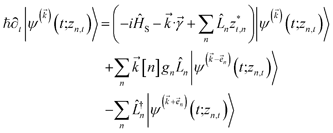 | (9) |
 to index auxiliary wave functions,
  is the nth element of the index vector,
  is the vector of correlation function exponents (γn), and terms involving any auxiliary wave function with an indexing vector containing a negative element are always zero. The linear HOPS equation maintains the normalization of the system reduced density matrix within the ensemble average, but the physical wave function is not normalized in individual trajectories. Instead, for long trajectories, most realizations have
  and an infinitesimal subset have physical wave functions with diverging norms.20 As a result, linear HOPS calculations exhibit slow convergence with respect to the size of the ensemble.
We can improve convergence with ensemble size by using the non-linear HOPS equation, which describes the time-evolution of a normalizable stochastic wave function. We rewrite the reduced system density matrix (eqn (5)) in terms of a normalized wave function and the norm contribution
 | (10) |
 . The norm in the first expression can be interpreted as a weighting factor for a new ensemble average. Using a Girsanov transform, we can solve for the corresponding equation-of-motion for |ψ(t;zn,t)〉,23 which gives the non-linear HOPS equation20
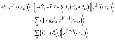 | (11) |
 | (12) |
 | (13) |
We note that the non-linear HOPS equation ensures that the contribution of each wave function is normalized in the reduced density matrix, but it time-evolves the non-normalized physical wave function. In the following, we will drop the explicit zn,t dependence from the wave function for simplicity  .
.
The HOPS equations are a numerically convenient, formally exact expression for exciton dynamics in small molecular aggregates. Moreover, the calculations are ‘embarrassingly’ (also called ‘perfectly’) parallel24 due to the independence of individual trajectories, and, as a result, HOPS ensembles can be computed using thousands of CPUs simultaneously without loss of efficiency. The application of HOPS to large molecular aggregates, however, is limited by the scaling of the HOPS basis with the number of molecules. It is convenient to think of HOPS calculations as depending on two basis sets: the state basis  and the auxiliary basis
  . The complete state basis is a finite set of vectors that span the Hilbert space of the system, while the complete auxiliary basis is composed of an infinite set of auxiliary wave functions indexed by vectors
  . To construct a finite auxiliary basis, the infinite hierarchy must be truncated. Here, we employ the common triangular truncation condition which limits the auxiliary basis to those wave functions with index vectors
  that have a sum of elements less than a preselected bound kmax
 . If we assume one independent environment per state, then the number of auxiliary wave functions included in the triangular truncation scales as
  which gives an overall
  scaling for large aggregates. While convergence as a function of kmax is guaranteed, the requisite number of auxiliary wave functions is often prohibitive.
Short-time correction and Markovian modes
The Drude–Lorentz correlation function given in eqn (4) has a discontinuity at t = 0 arising from the symmetry condition | (14) |
| αdl,n(t) = (Re[gn] + isgn(t)Im[gn])e−γn|t|/ℏ | (15) |
The discontinuity in the correlation function introduces a numerically inconvenient infinitely high-frequency component to the stochastic noise trajectories zn,t.
We ameliorate this problem by redefining the positive-time correlation function in terms of two continuous exponential functions α(t) = α0,n(t) + αmark,n(t) where
| α0,n(t) = gne−γn|t|/ℏ | (16) |
| αmark,n(t) = −iIm[gn]e−γmark|t|/ℏ. | (17) |
The definition of αmark,n(t) ensures the imaginary component of the total correlation is 0 when t = 0, and it also provides for a smooth transition back to the naive correlation function α0,n(t) on a finite timescale given by ℏ/γmark. Except where otherwise noted, γmark = 500 cm−1 for all calculations presented in the main text, because this was sufficiently fast to ensure the Markovian timescale had no influence on the calculated dynamics.
Due to the extremely rapid timescale on which αmark,n(t) decays, this mode is Markovian, and high-lying contributions to the hierarchy can be neglected. In the following, we will only include the first order terms associated with these Markovian modes and neglect these terms in our discussion of the auxiliary wave functions forming the hierarchy. This can be viewed as a smoothing of the noise trajectories (zn,t) on timescales fast compared to all other dynamics.
This problem can be avoided entirely by using a different spectral density which more naturally accounts for the short-time imaginary component of the correlation function: for example, the recently reported alternative to the Drude–Lorentz oscillator with improved low-temperature behavior.26
Adaptive HOPS (adHOPS)
Within the quantum state diffusion formalism, stochastic wave functions localize in the presence of thermal environments.27–29 At a single time point, the pure state can be interpreted as a system wave function conditioned on a measurement of all the environmental degrees-of-freedom.30 The delocalization extent of exciton wave functions within the ensemble of pure states is suppressed by the dynamic localization induced by coupling to the vibrational degrees-of-freedom.31,32 Previously, Markovian quantum state diffusion calculations have leveraged the locality of the exciton to reduce computational complexity using both a moving basis27,33 and an adaptive basis.34 Both of these approaches, however, require the conservation of probability, which is violated in the HOPS equations because amplitude in the auxiliary wave functions can be created and destroyed.Here, we develop an adaptive solution to the HOPS equation-of-motion that achieves size-invariant computational scaling (i.e.,  scaling) for calculations of large molecular aggregates. We first establish a normalized non-linear HOPS equation, which ensures that the magnitude of derivative terms does not diverge with increasing depth of the hierarchy. We then illustrate how locality appears within the hierarchy of auxiliary wave functions, with a particular emphasis on the connection between locality and the flux between neighboring auxiliary wave functions. Finally, we present an adaptive algorithm for the normalized non-linear HOPS equation that satisfies a user-selected bound on the absolute derivative error.
Normalization of HOPS
To ensure that the magnitude of the derivative elements for auxiliary wave functions have a consistent absolute scale across the hierarchy, we: (1) enforce normalization of the physical wave function in the time-evolution equation and (2) redefine the auxiliary wave function coefficients.To enforce the normalization of the physical wave function, we rewrite the non-linear HOPS equation in terms of a normalized physical wave function. Starting with eqn (11), dividing all wave functions by the norm of the physical wave function, taking the derivative, and expanding terms gives
 | (18) |
 | (19) |
In the non-linear HOPS equation, the magnitude of the auxiliary wave functions grows with increasing auxiliary index. The basic HOPS terminator for a hierarchy with a single thermal environment
 | (20) |
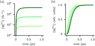
 increases with increasing auxiliary index which, given g/γ > 1, is consistent with the terminator condition. For a single mode hierarchy, we can ensure the norm of the auxiliary wave functions does not diverge by introducing a new k-dependent prefactor for each wave function (γ/g)k, as shown in Fig. 1b. In the multimode case, we extend the definition of the prefactor to
  which ensures that the auxiliary wave functions that define the edges of the hierarchy (only one non-zero mode) do not diverge with increasing hierarchy depth. Rewriting the non-linear HOPS equation to account for this additional prefactor leads to the normalized non-linear HOPS equation
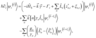 | (21) |
 | (22) |
Locality of HOPS
To construct an adaptive approach to solving the HOPS equations, we must first address the question: how and to what extent does the locality expected in the quantum state diffusion formalism appear in HOPS?
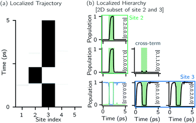
Fig. 2 shows that in HOPS calculations localization in the physical wave function induces localization in the hierarchy. By ‘localization in the hierarchy,’ we specifically refer to clustering of amplitude in a small set of auxiliary wave functions in a way that depends on the position of the excitation in the physical wave function. In Fig. 2a, an excitation begins on the middle site of a five pigment chain and then jumps between site 3 and site 2. Fig. 2b plots the norm of auxiliary wave functions associated with site 2 and site 3; each plot is labeled by an auxiliary vector index  . For example, [0,1,0,0,0] (Fig. 2b, first column) is the first order auxiliary wave function associated with the thermal environment on the second site. The occupation of the auxiliary wave functions (black lines, Fig. 2b) track with the population of the physical wave function – i.e., the auxiliary wave functions associated with the thermal environment of site 2 (first column Fig. 2b) are only occupied when site 2 is occupied in the physical wave function (shaded region).
The locality in the HOPS hierarchy can be understood in terms of the balance of flux terms in the normalized non-linear HOPS equation. First, every auxiliary wave function is damped (first line of eqn (21),  ) and, therefore, has zero amplitude without a continuous source term. The fundamental source term is the physical wave function which is the lowest order of the hierarchy. The flux of amplitude towards higher-lying auxiliary wave functions arises from the second line of eqn (21)
 . For system-bath coupling operators that are site projection operators
  , the flux towards higher-lying auxiliaries only arises when there is amplitude on the associated site of the lower auxiliary wave function. Moreover, the auxiliary wave functions are localized by the same dynamics that localize the physical wave function. As a result, the localized auxiliary wave functions only contribute amplitude to higher-lying auxiliary wave functions with an index that differs by
  in a site (n) with non-zero amplitude. Thus, the locality of the physical wave function results in preferential population of specific auxiliary wave functions.
Adaptive algorithm
We have developed an adaptive algorithm for time-evolving the HOPS equations (adaptive HOPS, adHOPS) that leverages locality by constructing a reduced basis set at each time point. We establish the essential basis set elements at each time point (t) by ensuring that the error in the time-derivative introduced by the truncated auxiliary and state
  basis is below a given threshold (δ). We define the derivative error in terms of Euclidean distance between the true derivative vector and the effective derivative vector constructed using the adaptive basis. The key equations (given in the ESI†) provide an upper bound on the derivative error squared and are derived by considering all possible flux contributions in the normalized non-linear HOPS equation (eqn (21)), excluding higher order effects introduced through the normalization correction (Γt). Because auxiliary wave functions share only nearest neighbor connections
  and the Hamiltonian for a molecular aggregate supports electronic couplings over a finite spatial extent, the adaptive basis can be constructed with
  scaling. The result is a calculation where, in addition to a trajectory of the wave functions, we construct an adaptive basis-set trajectory
  where
where  .
.
Our adHOPS algorithm neither assumes nor imposes locality. Rather, the adaptive basis takes advantage of whatever locality arises during the simulation. If the full hierarchy is required to satisfy the derivative error bound, adHOPS smoothly reverts to a HOPS calculation. As a result, adHOPS remains formally exact – the adaptive basis represents a time-dependent truncation of hierarchy elements, and δ, like kmax, is a convergence parameter.
We note that the current adHOPS algorithm makes use of two approximations: first, the spectral density is assumed to be over-damped (e.g., Drude–Lorentz), which allows for a consistent normalization of the hierarchy elements. Second, the system-bath coupling operator is assumed to be a site-projection operator (![[L with combining circumflex]](https://www.rsc.org/images/entities/i_char_004c_0302.gif) n = |n〉〈n|); in other words, we assume that each molecule has an independent vibrational environment.
n = |n〉〈n|); in other words, we assume that each molecule has an independent vibrational environment.
Results and discussion
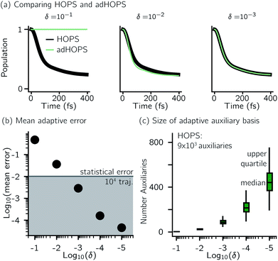
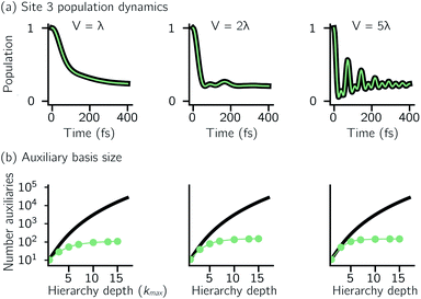
For a five-site linear chain, adHOPS calculations converge rapidly with respect to the derivative error bound and require only a small fraction of the full HOPS basis. Fig. 3a shows the comparison between full (black line) and adaptive (green line) HOPS population dynamics of the initially excited pigment (site 3). For δ = 10−1, the adaptive basis set is so small that the calculation shows no excitation transport. Smaller values of δ improve the description, and by δ = 10−3 the mean error is less than 10−2. Fig. 3b shows the mean adaptive error as a function of δ. In the grey region the adaptive error is smaller than the statistical error associated with the 104 trajectory ensemble. We measure the size of the auxiliary basis for a single trajectory by the average number of auxiliary wave functions required across time points. Fig. 3c plots the ensemble distribution of the auxiliary basis size as a function of δ. For δ = 10−3, most adHOPS trajectories require 102 auxiliaries on average, or approximately 1% of the 9 × 10³ auxiliaries required for the corresponding HOPS calculation. Improving the accuracy of the calculation by decreasing δ two orders of magnitude only requires about four times as many auxiliaries. The other kinds of error that arise in HOPS simulations, including statistical error from a finite number of trajectories and hierarchy error from the finite kmax value, are reported in the ESI.†One persistent challenge for numerical implementations of formally exact methods is demonstrating the calculations are converged to the exact answer. In hierarchical methods, calculations must be converged with respect to the auxiliary basis which is defined in the triangular truncation condition by the maximum hierarchy level considered (kmax). In HOPS, the criterion for convergence is that kmaxγ/ℏ ≫ ωs, where ωs is the characteristic frequency of the system.20 Because the full auxiliary basis scales as  , it is often impractical to systematically check convergence for sufficiently large values of kmax. Though our adHOPS method was inspired by localization, we find that it naturally incorporates a dynamic filtering scheme that dramatically improves the scaling of the auxiliary basis with kmax even when the exciton is fully delocalized. Fig. 4a compares the full (black) and adaptive (green) HOPS dynamics with increasing coupling (V). By V = 5λ the oscillations in the site 3 population report a wave function that is coherently oscillating across 5 sites. Fig. 4b shows the corresponding size of the auxiliary basis as a function of kmax. In all cases the adaptive auxiliary basis (green line) increases much more slowly than the full auxiliary basis (black line).
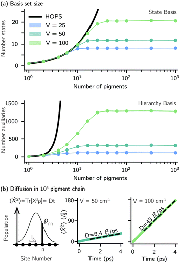
Another perpetual challenge for formally exact methods is their intractable computational scaling with the number of molecules. In HOPS calculations this arises from the scaling of the auxiliary basis. Fig. 5a compares the full (black line) size of the state (top) and auxiliary (bottom) basis to the average size of the adaptive basis (colored lines) as a function of the number of molecules in a linear chain. Compared to the full auxiliary basis, the size of the adaptive auxiliary basis scales favorably with respect to the number of molecules in the aggregate. Moreover, both the auxiliary and state bases in adHOPS calculations show a plateau beyond a threshold size of the linear chain (Npig > N*), indicating the onset of size invariant scaling. In the ESI,† we compare the CPU time required for full and adaptive HOPS calculations (V = 50 cm−1). We find that adaptive calculations are faster than full calculations starting around Npig = 10, and we also demonstrate the onset of size invariance (i.e.,  ) scaling of CPU time for large aggregates. In other words, increasing the number of pigments beyond a threshold size does not increase the computational expense of an adHOPS calculation. Thus, for localized excitons, the size invariance of adHOPS allows for calculations on scales that were previously unachievable for formally exact methods.
Our adaptive HOPS algorithm offers a computationally tractable approach for formally exact calculations of mesoscale quantum dynamics. As a proof-of-concept, we demonstrate the ability to simulate exciton diffusion on a linear chain of 103 molecules within the formally exact framework of adHOPS (Fig. 5b). Exciton diffusion is a common experimental observable extracted from non-linear microscopies2 but is challenging to simulate on long length scales.35–37 Using adHOPS, simulating exciton diffusion in a linear chain of 103 pigments is computationally tractable because for V = 100 cm−1 it requires, on average, less than 2 × 10³ auxiliary wave functions and 20 pigment states. The corresponding HOPS simulation would require an auxiliary basis containing more than 1023 auxiliary wave functions.
Conclusions
To summarize, our adaptive HOPS (adHOPS) algorithm:1. Is a formally exact solution to the time-evolution of a quantum state coupled to a non-Markovian thermal reservoir,
2. Is embarrassingly (or ‘perfectly’) parallel,24 and
3. Achieves size-invariant (i.e.,  ) scaling for molecular aggregates that are substantially larger than the exciton delocalization extent in the material.
This combination of properties allows us to perform non-perturbative, non-Markovian simulations involving an arbitrary number of pigments in physically relevant parameter regimes, thus laying the foundation for mesoscale quantum dynamics simulations of excited-state carriers in molecular materials. Currently, our adaptive algorithm assumes that each pigment has an independent thermal environment composed of overdamped vibrations, but future developments will allow for a broader class of mechanisms involving high-frequency intra-molecular vibrations38–40 and Peierls-type electron-vibration coupling.3 Looking forward, we believe that adHOPS provides a promising new direction for simulations of a broad range of organic semiconductors including photosynthetic membranes,16,41 molecular thin films,42,43 and organic photovoltaic heterojunctions.17–19,44
Data availability
The data that supports the findings of this study, the scripts used to run calculations, and the code required to generate the figures are available at DOI: 10.5281/zenodo.4597068. The most recent release of MesoHOPS is available through GitHub at https://github.com/MesoscienceLab/mesohops. The source code used for these calculations is available at DOI: 10.5281/zenodo.4592583.Author contributions
Investigation, software, writing – LV, JKL, DIGB; formal analysis, visualization – LV, JKL; conceptualization, funding acquisition, supervision – DIGB.Conflicts of interest
There are no conflicts to declare.Note added after first publication
This version replaces the manuscript published on 17th June 2021 which contained errors in the application of proof corrections impacting several of the mathematical equations. The RSC apologises for any confusion.Acknowledgements
We thank the Robert A. Welch Foundation (Grant N-2026-20200401) and start-up funds from SMU for financial support. DIGB thanks Alex Eisfeld, Richard Hartmann, and Walter Strunz for insightful conversations.Notes and references
- M. Delor, H. L. Weaver, Q. Yu and N. S. Ginsberg, Nat. Mater., 2020, 19, 56–62 CrossRef CAS PubMed.
- N. S. Ginsberg and W. A. Tisdale, Annu. Rev. Phys. Chem., 2020, 71, 1–30 CrossRef CAS PubMed.
- T. Nematiaram and A. Troisi, J. Chem. Phys., 2020, 152, 190902 CrossRef CAS PubMed.
- M. Yang and G. R. Fleming, Chem. Phys., 2002, 18, 163–180 CrossRef.
- J. Schulze, M. F. Shibl, M. J. Al-Marri and O. Kühn, J. Chem. Phys., 2016, 144, 185101 CrossRef PubMed.
- H. Wang and M. Thoss, J. Chem. Phys., 2003, 119, 1289–1299 CrossRef CAS.
- D. Tamascelli, A. Smirne, J. Lim, S. F. Huelga and M. B. Plenio, Phys. Rev. Lett., 2019, 123, 090402 CrossRef CAS PubMed.
- Y. Tanimura, J. Chem. Phys., 2020, 153, 020901 CrossRef CAS PubMed.
- N. Makri, Chem. Phys. Lett., 1992, 193, 435 CrossRef CAS.
- T. Kramer, M. Noack, J. R. Reimers, A. Reinefeld, M. Rodríguez and S. Yin, Chem. Phys., 2018, 515, 262–271 CrossRef CAS.
- T. Kramer, M. Noack, A. Reinefeld, M. Rodríguez and Y. Zelinskyy, J. Comput. Chem., 2018, 39, 1779–1794 CrossRef CAS PubMed.
- N. Makri, J. Chem. Phys., 2018, 149, 214108 CrossRef PubMed.
- N. Makri, J. Chem. Phys., 2018, 148, 101101 CrossRef PubMed.
- A. D. Somoza, O. Marty, J. Lim, S. F. Huelga and M. B. Plenio, Phys. Rev. Lett., 2019, 123, 100502 CrossRef CAS PubMed.
- D. Balzer, T. J. A. M. Smolders, D. Blyth, S. N. Hood and I. Kassal, Chem. Sci., 2021, 12, 2276–2285 RSC.
- K. Amarnath, D. I. G. Bennett, A. R. Schneider and G. R. Fleming, Proc. Natl. Acad. Sci. U.S.A., 2016, 113, 1156–1161 CrossRef CAS PubMed.
- S. N. Hood and I. Kassal, J. Phys. Chem. Lett., 2016, 7, 4495–4500 CrossRef CAS PubMed.
- A. E. Jailaubekov, A. P. Willard, J. R. Tritsch, W.-L. Chan, N. Sai, R. Gearba, L. G. Kaake, K. J. Williams, K. Leung, P. J. Rossky and X.-Y. Zhu, Nat. Mater., 2013, 12, 66–73 CrossRef CAS PubMed.
- N. R. Monahan, K. W. Williams, B. Kumar, C. Nuckolls and X.-Y. Zhu, Phys. Rev. Lett., 2015, 114, 247003 CrossRef PubMed.
- D. Suess, A. Eisfeld and W. T. Strunz, Phys. Rev. Lett., 2014, 113, 150403 CrossRef CAS PubMed.
- A. Ishizaki and G. R. Fleming, J. Chem. Phys., 2009, 130, 234111 CrossRef PubMed.
- L. Diosi and W. T. Strunz, Phys. Lett. A, 1997, 235, 569–573 CrossRef CAS.
- L. Diosi, N. Gisin and W. T. Strunz, Phys. Rev. A, 1998, 58, 1699–1712 CrossRef CAS.
- M. Herlihy, N. Shavit, V. Luchangco and M. Spear, The art of multiprocessor programming, Newnes, 2020 Search PubMed.
- V. May and O. Kühn, Charge and energy transfer dynamics in molecular systems, John Wiley & Sons, 2008 Search PubMed.
- A. Ishizaki, J. Phys. Soc. Jpn., 2020, 89, 015001 CrossRef.
- R. Schack, T. A. Brun and I. C. Percival, J. Phys. A: Math. Gen., 1995, 28, 5401–5413 CrossRef.
- N. Gisin and I. C. Percival, J. Phys. A: Math. Gen., 1993, 26, 2233–2243 CrossRef.
- N. Gisin and I. C. Percival, J. Phys. A: Math. Gen., 1993, 26, 2245–2260 CrossRef.
- J. Gambetta and H. M. Wiseman, Phys. Rev. A, 2002, 66, 012108 CrossRef.
- R. Monshouwer, M. Abrahamsson, F. van Mourik and R. van Grondelle, J. Phys. Chem. B, 1997, 101, 7241–7248 CrossRef CAS.
- M. Dahlbom, T. Pullerits, S. Mukamel and V. Sundström, J. Phys. Chem. B, 2001, 105, 5515–5524 CrossRef CAS.
- R. Schack, T. A. Brun and I. C. Percival, Phys. Rev. A, 1996, 53, 2694–2697 CrossRef CAS PubMed.
- X. Gao and A. Eisfeld, J. Chem. Phys., 2019, 150, 234115 CrossRef PubMed.
- S. K. Saikin, M. A. Shakirov, C. Kreisbeck, U. Peskin, Y. N. Proshin and A. Aspuru-Guzik, J. Phys. Chem. C, 2017, 121, 24994–25002 CrossRef CAS.
- M. Delor, A. H. Slavney, N. R. Wolf, M. R. Filip, J. B. Neaton, H. I. Karunadasa and N. S. Ginsberg, ACS Energy Lett., 2020, 1337–1345 CrossRef CAS.
- Y. Wan, Z. Guo, T. Zhu, S. Yan, J. Johnson and L. Huang, Nat. Chem., 2015, 7, 785–792 CrossRef CAS PubMed.
- S. Bera, N. Gheeraert, S. Fratini, S. Ciuchi and S. Florens, Phys. Rev. B: Condens. Matter Mater. Phys., 2015, 91, 041107 CrossRef.
- S. M. Blau, D. I. G. Bennett, C. Kreisbeck, G. D. Scholes and A. Aspuru-Guzik, Proc. Natl. Acad. Sci. U.S.A., 2018, 115, E3342–E3350 CrossRef CAS PubMed.
- D. I. G. Bennett, P. Malý, C. Kreisbeck, R. van Grondelle and A. Aspuru-Guzik, J. Phys. Chem. Lett., 2018, 9, 2665–2670 CrossRef CAS PubMed.
- C. MacGregor-Chatwin, M. Sener, S. F. Barnett, A. Hitchcock, M. C. Barnhart-Dailey, K. Maghlaoui, J. Barber, J. A. Timlin, K. Schulten and C. N. Hunter, Plant Cell, 2017, 29, 1119–1136 CrossRef CAS PubMed.
- D. H. Arias, K. W. Stone, S. M. Vlaming, B. J. Walker, M. G. Bawendi, R. J. Silbey, V. Bulović and K. A. Nelson, J. Phys. Chem. B, 2013, 117, 4553–4559 CrossRef CAS PubMed.
- S. Sharifzadeh, P. Darancet, L. Kronik and J. B. Neaton, J. Phys. Chem. Lett., 2013, 4, 2197–2201 CrossRef CAS.
- K. B. Whaley, A. A. Kocherzhenko and A. Nitzan, J. Phys. Chem. C, 2014, 118, 27235–27244 CrossRef CAS.
Footnote |
| † Electronic supplementary information (ESI) available: PDF contains the explanation of the statistical, hierarchy, and time-step errors; the expressions for evaluating derivative error terms; description of the adaptive error distribution in the ensemble; CPU timing data for adHOPS calculations. See DOI: 10.1039/d1sc01448j |
| This journal is © The Royal Society of Chemistry 2021 |

