Classification of crystal structures using electron diffraction patterns with a deep convolutional neural network

Abstract

Investigations have been made to explore the applicability of an off-the-shelf deep convolutional neural network (DCNN) architecture, residual neural network (ResNet), to the classification of the crystal structure of materials using electron diffraction patterns without prior knowledge of the material systems under consideration. The dataset required for training and validating the ResNet architectures was obtained by the computer simulation of the selected area electron diffraction (SAD) in transmission electron microscopy. Acceleration voltages, zone axes, and camera lengths were used as variables and crystal information format (CIF) files obtained from open crystal data repositories were used as inputs. The cubic crystal system was chosen as a model system and five space groups of 213, 221, 225, 227, and 229 in the cubic system were selected for the test and validation, based on the distinguishability of the SAD patterns. The simulated diffraction patterns were regrouped and labeled from the viewpoint of computer vision, i.e., the way how the neural network recognizes the two-dimensional representation of three-dimensional lattice structure of crystals, for improved training and classification efficiency. Comparison of the various ResNet architectures with varying number of layers demonstrated that the ResNet101 architecture could classify the space groups with the validation accuracy of 92.607%.

---

1. Introduction

Many of the fundamental materials properties originate from the interatomic bonding and the way the lattice atoms are arranged in unit cells.¹ These properties as reflected in the property tensors and band structures of crystalline materials lie in the symmetries of the unit cells. The crystal symmetry, starting from the seven crystal systems, can be broken down to the 230 space groups via the 32 crystal classes corresponding to the 32 point groups, in accordance with appropriate symmetries.² Identification and classification of the crystal structure, the starting point of investigating the structure–property relations, is the process of assigning any given materials system to one of these space groups and/or crystal classes, usually assisted by diffraction techniques.³ Various beam sources are incident on materials samples under investigation. The beams are then diffracted by the crystallographic planes inside the materials, generating material-specific signals recorded in one-dimensional (1D) diffractograms such as X-ray diffraction (XRD) patterns or two-dimensional (2D) geometric patterns such as selected area diffraction (SAD) patterns and electron backscatter diffraction (EBSD) patterns.³

The diffraction patterns containing the symmetry information of materials are the results of interaction between the incident beam represented by the wave vector and the samples' crystal structures reconstructed as reciprocal lattices, generating geographic relations between the beam direction, sample orientation, and particular crystallographic planes.³ Additionally, there exist selection rules determining which crystallographic planes should be absent in the diffraction patterns.³ Analysis of the diffraction data and extracting the crystallographic information from them inevitably require in-depth knowledge of crystallography and expertise as well as experiences. Although a high-throughput diffraction measurement method has been developed,⁴ analyzing diffraction data for materials characterization is still a time-consuming task even for expert crystallographers.

When any work requires high level of expertise including many years of experiences and complicated processes, it can be facilitated with the aid of computers. In the field of crystallography, computer-aided techniques have been in use especially when analyzing XRD or SAD patterns.^5–8 However, the process is not fully automated, and the analysis of diffraction data still requires guess work and computer simulations based on experiences and in-depth knowledge. If the material of interest is an unknown type as happens in the development of novel materials or if no prior material information is available, the process becomes more complicated. Recent advances in artificial intelligence (AI), assisted by ever-increasing computing power at lower costs, suggest possibilities of simplifying the analysis by non-experts. Deep learning techniques have been adopted to analyze domain-specific data due to its accurate prediction capabilities. More specifically, useful techniques including dropout⁹ and residual learning¹⁰ allow the construction of fast and accurate deep neural networks which show better performances than human in some areas.¹¹ Concerning the diffraction patterns, recent studies include analysis of both the 1D and the 2D patterns. It has been demonstrated that convolutional neural network, coupled with large amount of powder XRD pattern data, could classify the space group, extinction group, and crystal system with the accuracy levels of 81.14, 83.83, and 94.99%, respectively using about 150 000 XRD data with no feature engineering involved.¹² In this work, the XRD pattern data in pristine forms were used to train a convolutional neural network (CNN). In another approach, it was possible to develop a supervised machine learning framework, which enabled the analysis of XRD pattern for the case where only sparse dataset are available.¹³ It has also been demonstrated that CNN and feedforward neural network (FFNN) could classify the XRD patterns with reasonable accuracies (higher than 80%).¹⁴ There was an interesting approach, in which 1D diffraction intensity profile dataset was prepared by converting 2D patterns obtained by fast Fourier transformation of the high-resolution (HR) scanning transmission electron microscope (STEM) images.¹⁵ This suggests that 2D patterns can be classified once they are converted to 1D profiles.

Attempts have also been made to classify 2D diffraction patterns. Kaufmann et al.¹⁶ have suggested two CNN models that can identify the Bravais lattice or the space group of unknown materials from their EBSD patterns with the accuracies of 93.5% and 91.2%, respectively. Ziletti et al.¹⁷ have developed a CNN-based method which used indexed diffraction pattern images to classify the lattice symmetry. In this work, they prepared dataset by superposing and color-indexing the 6 images for a material which were obtained by simulating beam diffraction incident on a virtual sample along three crystal axes. Although the images contain regular array of diffraction spots, they were different from SAD patterns (SADPs) since only three principal crystal axes were used as the beam directions (BDs) and that the diffraction patterns were color-indexed and then superposed. Since XRD, EBSD, and SAD are mutually complimentary, AI-assisted classification of SADPs would be worth exploration.

Inspired by the work of Ziletti et al., this study has been carried out for the classification of crystal symmetry in terms of the space group from 2D diffraction patterns that resemble real SADPs obtained by aligning BDs to various zone axes in transmission electron microscopy (TEM). As a starting point, the cubic system was considered. This system contains 36 space groups and covers many materials systems familiar to materials scientists and engineers.^2,18 To improve the training and classification efficiency, the diffraction pattern dataset was regrouped and labeled from the viewpoint of computer vision, i.e., the way how the machine ‘sees’ the patterns. Instead of developing a dedicated DCNN architecture, a well-established off-the-shelf image classification architecture, residual neural network (ResNet),¹⁰ was adopted. For the space groups 213, 221, 225, 227, and 229, the ResNet101 model showed the prediction accuracies of 92.607%. The overall workflow is schematically illustrated in Fig. 1 together with the classification structure of the ResNet architecture.

Fig. 1 Schematics illustrating (a) the overall sequence of the crystal structure classification proposed in this study and (b) the inner working of the ResNet architecture.

2. Dataset

2.1 Model systems and data mining

It is hard to expect that the ResNet architecture has an omnipotent SADP classification capability. Hence, the work began with the cubic system which has the highest symmetry and contains many materials systems familiar to the science and engineering communities.^2,18 Once proven successful, it is expected that the scheme can be extended to other crystal systems in the sequence of decreasing symmetry, namely in the order of hexagonal, rhombohedral, tetragonal, orthorhombic, monoclinic, and triclinic systems. Among 36 space groups (from 195 to 230) in the cubic systems, space groups 213, 221, 225, 227, and 229 were chosen based on the distinguishability of SADPs, which is discussed in the following subsection. Once the model system is chosen, it is necessary to prepare the dataset for training the neural network and for validating its prediction accuracy.

The dataset should be in a standard format with the same resolution and be available in large quantity (usually dataset consists of tens of thousands of images or more). Since these requirements cannot be met by experimental acquisition of the SADPs and/or by collection of the SADPs published in literature, the dataset resembling the TEM SADPs were generated by a computer simulation in a systemized way in this study. The material information inputs for the diffraction simulation were provided via crystal information format (CIF). The CIF files were obtained from the open database repositories Materials Project¹⁹ and AFLOWLIB.^20,21 The CIF files in these repositories are experimentally obtained and/or theoretically calculated and many of them are also deposited in Inorganic Crystal Structure Database (ICSD).²² On average, 49.8 CIF files for each space group to be considered were collected and used as inputs for the diffraction simulation.

2.2 Electron diffraction simulation

Number of software packages are available for the simulation and analysis of electron diffraction: JEMS,²³ QSTEM,²⁴ Landyne Software Suite,²⁵ SingleCrystal,²⁶ etc. for example. These software packages provide user-friendly interfaces and have many functionalities. On the other hand, they are not fully automated and not suitable to generate large number of diffraction patterns required to train the neural network in reasonable time at reasonable cost. In the absence of fully automated simulation tools, an open-source package Condor²⁷ was adapted to prepare the simulated electron diffraction pattern images that resemble the SADPs. While the Condor package was designed to simulate the diffraction of flash X-ray, preliminary tests showed that they can also be used to simulate the electron diffraction with minor modifications. Modifications of Condor here include the followings: (i) generation of virtual single crystals by replicating the unit cell information provided by the input CIF files as required by the users; (ii) automatic alignment of the zone axes of the virtual crystal along the direction of the incident beam as intended by the users; (iii) selection of the electron wavelength by varying the acceleration voltage with the relativistic corrections; (iv) normalization of the intensity of the diffracted beams with respect to the highest intensity as appear in the brightness of the diffraction spots in the simulated images; and (v) assumption of the three-dimensional Gaussian distribution of the intensity of the incident electron beams.

Normalization of the diffracted beam intensity was necessary since the neural network was designed to recognize relative differences in the intensities of the diffraction spots in the images. Three-dimensional Gaussian wave assumption was used to simulate the blurring of the edges of the diffraction spots in real SADPs, despite the plane-waves assumption of the incident electron beam is used in TEM diffraction theories.^2,31 Use of the three-dimensional Gaussian beam was also effective in eliminating the effect of sample shapes and sizes especially when the virtual crystal is small compared with real samples used in experiments. The simulated diffraction patterns were formed as portable graphics format (PNG) images consisting of 256 × 256 pixels. This image size was chosen to minimize the computing resource requirements for image generation while enabling the meaningful recognition and classification of images by the neural network. Examples of the simulated SADPs for Si (space group 227) herein with varying BDs are shown in Fig. 2. These simulated images were comparable to the real SADPs reported in the literature^28–30 in that: (i) the simulated SADPs include relative differences in the brightnesses of the diffraction spots; and (ii) individual diffraction spots have Gaussian distribution of the intensity from its center to the edge while the edge itself is blurry like the real ones, indicating that the simulation by the modified Condor was suitable to generate the SADP-like dataset.

Fig. 2 Examples of the simulated SADP-like diffraction images generated for Si (space group 227) with (a) BD = [001], (b) BD = [011], (c) BD = [111], and (d) BD = [103]. These simulated patterns were comparable to the experimentally obtained SADPs reported elsewhere^28–30 (the real SADPs are not shown due to the copyright related issues).

3. Space group classification by deep learning

3.1 Data regrouping for training AI

The SADPs are 2D representations of 3D atomic configuration in reciprocal spaces. Inevitably, a single SADP obtained for one beam direction (BD) corresponding to a specific zone axis does not include all the symmetry information pertaining to the space group of the material under investigation. Further, overlapping diffractions may be obtained from two different materials belonging to different space groups. For example, one material in the space group 225, CeTe, and the other material in the space group 227, LiGa, can show indistinguishable SADPs if the BD is aligned to [001] zone axis. Another example is the case of the SADPs for CeTe with BD = [111] and for Co (space group 194 in the hexagonal system) with BD = [001]. These examples are shown in Fig. 3a through 3d. Usually, materials scientists utilize number of SADPs obtained with varying zone axes to analyze the crystal structure of any given material. Even in such a case, not all space groups can be distinguished using SADPs. For example, SADPs for the materials in the space groups 197 and 229 always overlap when the same BD is applied to obtain the SADP for each space group. Meanwhile, diffraction patterns for some materials in the same space group are apparently different in that diffraction spots corresponding to the same crystallographic planes show some differences in their intensities (brightnesses). For instance, the SADPs with BD = [112] for LiGa and for Zr₄Pt₂N (space group 227) look different although the diffraction spots have the same arrangements as shown in Fig. 3e and f. In fact, the choice of space groups 213, 221, 225, 227, and 229 among 36 space groups in the cubic system in this study is based on the similarity of the diffraction patterns as mentioned herein. The space group 213 shares similar diffraction patterns with the space group 212; 221 with 195, 200, and 215; 225 with 196, 202, and 216; 229 with 197, 199, 204, 211, and 217. In the case of space group 227, appearances of the diffraction patterns suggest that it can be divided into three sub-groups.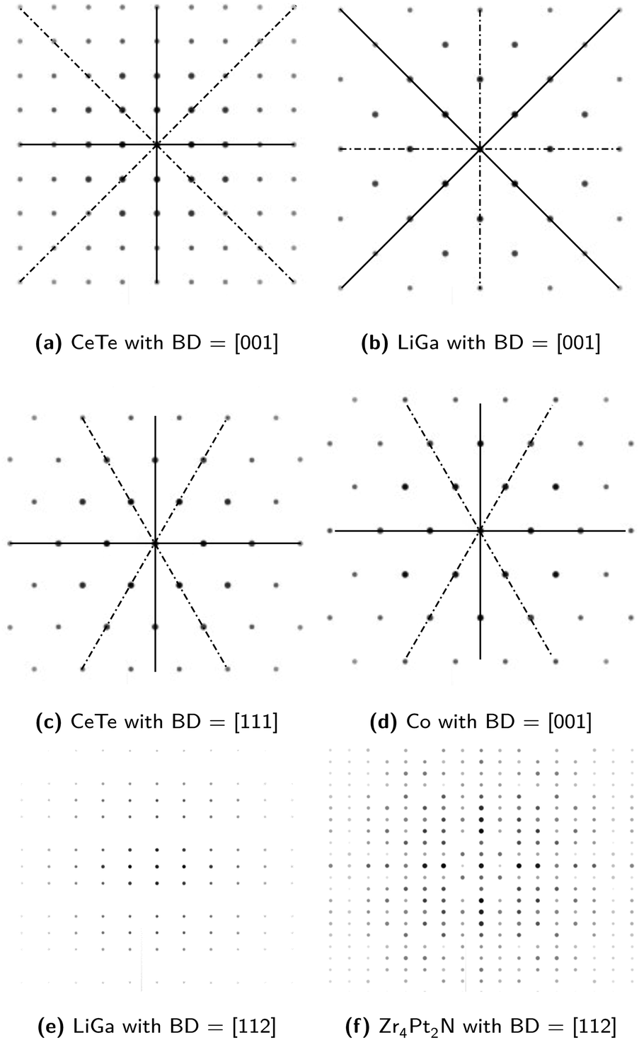

Fig. 3 Examples of (a) & (b) the similar diffraction patterns with the same zone axis obtained for the materials belonging to different space groups while sharing the same crystal system; (c) & (d) similar diffraction patterns with the different zone axes obtained for the materials belonging to different space groups and crystal systems; and (e) & (f) apparently different diffraction patterns with the same zone axis obtained for the materials sharing the same space group. These diffraction patterns were simulated using JEMS²³ and CIF files from Materials Project¹⁹ repository.

Concerning the adoption of the DCNN algorithm for crystal structure classifications, the axiom is that what is indistinguishable to humans is also indistinguishable to machines. Therefore, grouping the diffraction pattern data by the space group and the zone axis (or BD aligned to it) and labeling them accordingly is not suitable to train the neural network, not to mention the humans, if it is intended that the data be classified only through the images without any knowledge of crystallography and geometry and any information regarding the material system of interest. What the machine does is to sort and classify the input data only by the ‘appearance’, viz. pixel by pixel information. Therefore, necessity arises as to how the diffraction patterns should be regrouped and labeled to train the DCNN architecture. This regrouping and labeling scheme will be referred to as ‘dataset class labeling’ hereinafter.

The dataset class labeling scheme herein is based on how the diffraction patterns ‘look’ to human as well as to the machine. Noting that the diffraction pattern is the 2D periodic array of the diffraction spots, one may expect that the diffraction patterns can be matched to five 2D lattice systems dealt with in crystallography.³² Accordingly, the diffraction patterns are regrouped to four of these five systems, namely square primitive (square, category A), rectangular primitive (rectangle, category B), hexagonal primitive (rhombus, category C), and oblique primitive (parallelogram, category D). Rectangular centered system was merged to oblique primitive lattice since the former can also be described as the latter.

In the cubic crystal system, the SADPs for the 〈100〉 zone axis are square and those for the 〈111〉 zone axis are hexagonal. On the other hand, those for other zone axes will be rectangular or parallelogrammatic with varying side lengths and angle between the sides depending on the zone axes. When an SADP forms a rectangular primitive lattice, its zone axis can be identified by the relative lengths of two intersecting sides. This length ratio can be represented by the angle between a diagonal and a principal axis as illustrated with an example SADP in Fig. 4a. Hence, this angle can be used to identify whether two (or more) patterns look the same or different. If an SADP forms an oblique primitive lattice, differences in zone axis will be reflected in the relative lengths of two intersecting sides of the primitive cell and the angle between them. The parallelogram can be partitioned into two triangles, and the two angles of a triangle, namely ∠BOA and ∠OAB in Fig. 4b shown with an example SADP, can represent the geometric features of the parallelogram. Once the sequence of these two angles is also included, they can be used to distinguish zone axis of a diffraction pattern including the chirality. While the diffraction spots form specific regular arrays, they can show difference in intensities (brightnesses). Often, some of the diffraction spots are absent depending on the combination of the Miller indices for a plane (h, k, and l), which also possesses some regularity. This feature can also be used to classify the dataset. Now, there are three criteria for the dataset class labeling. First, the arrangement of diffraction spots in the SADPs are used to assign any pattern to four primary groups classified as A, B, C, and D by the primitive lattice shapes as mentioned above. Next, the angle information described above is used to subdivide the primary group into sub-groups. These sub-groups are designated by numbers following the primary group designation characters. Finally, the sub-group is partitioned in accordance with the patterns of the absence and the relative intensities of the diffraction spots. These partitions are denoted as numbers following a hyphen. One example of these regrouping and labeling scheme is illustrated in Fig. 5.

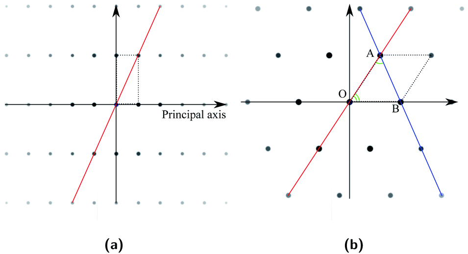Fig. 4 Examples of SAD patterns matched to 2D lattice: (a) for BaSe (space group 225) with BD = [102] matched to a rectangle and (b) for BaSe with BD = [214] matched to a parallelogram. The angles defining the geometric feature of the patterns are marked in these patterns.

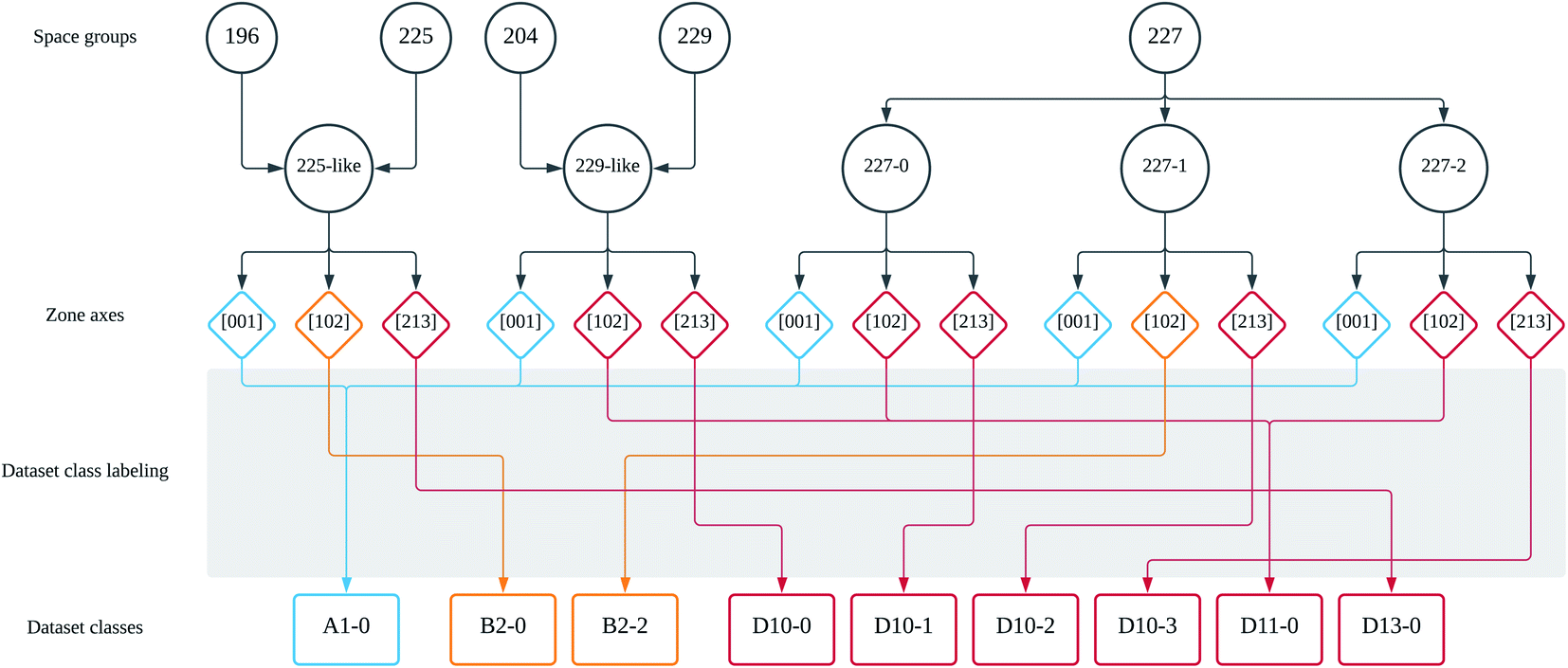Fig. 5 Schematic illustrating the structure of the dataset labeling scheme developed in this study.

As a result of the application of the above labeling scheme, the number of dataset classes decreased substantially. For the example shown in Fig. 5, there can be 15 dataset classes by crystallography. Compared with this, regrouping by using the 2D-pattern-based dataset labeling scheme reduced them to 9 dataset classes. This decrease helps improving the training efficiency of the neural network, because confusing classes (space groups 225 with BD = [001] and 227 with BD = [001] for example) due to the indistinguishable diffraction patterns are merged into the same new class label (A1-0 in this example case). Now the neural network can compare the input SADPs obtained for several zone axes with the regrouped class labels. Combinations of the regrouped class label will lead to a specific space group by the ensemble of the probability result for each SADP. This procedure is further discussed in 3.2. For the five space groups considered in this study (in fact, the space group 227 may contain 3 effective space groups based on the SADPs considering the brightness of the diffraction spots), the SADPs were generated with respect to 16 zone axes. In terms of crystallography, this leads to 112 dataset classes. However, once the 2D-pattern-based dataset class labeling scheme herein is applied, this was reduced to 60. It is emphasized that this is not only a simple reduction in number but also a dataset restructuring with the dataset labeling scheme as stated in this section for efficient classification to be performed by the ResNet architectures!

3.2 Space group classifications

Using the dataset as regrouped by the labeling scheme described above, five ResNet architectures with different sizes (different number of layers) were trained and then tested to verify whether they can predict the space group of a material using SADPs with varying zone axes. The ResNet architectures used herein include ResNet18, ResNet34, ResNet50, ResNet101, and ResNet152. One advantage of ResNet architecture associated with its residual block is that increasing the number of layers does not induce a vanishing gradient problem which hinders a training process for a deep network.^10,33 Before training these architectures, entire CIF files were first split into the training set and the validation set separately at a ratio of 8.5 to 1.5. Subsequently, SADP-like patterns were simulated using the modified Condor package, generating 68 480 images for the training set and 11 200 images for the validation set, respectively. When it comes to real diffraction pattern images, the patterns may have different scales, may be randomly rotated with respect to the BDs, or may be off-centered, i.e., the (000) position is not located in the image center. To help the ResNet architectures cope with these variations in images thereby improving a generalization capability, data augmentations were carried out by transforming geometries of the simulated SADPs. Differences in scales of the diffraction patterns were considered by generating the simulated images with varying camera lengths and acceleration voltages (wavelengths of the electron beams). For the random rotation issues, each SADP was rotated with the angles from 0 to 30 degrees about image surface normal direction. For the off-centering problems, the original 256 × 256-pixel simulated images were randomly cropped with 224 × 224-pixel resolutions. Examples of these dataset augmentation are shown in Fig. 6.

Fig. 6 Examples of the dataset augmentation to reflect irregularities in the SADPs obtained from real experiments: (a–c) scaling by changing the camera length; (d–f) of rotations; and (g) random cropping.

To train the ResNet architectures, two paradigms can be considered. One is the training from scratch, in which the neural network starts to update the model weights from randomly initialized weight and uses mostly target dataset (simulated SADPs) during the training process. The other is the fine-tuning, in which the neural network starts to update the model weights from the existing model, called pre-trained model, that was trained to solve different problems.^34,35 Typically, pre-trained model is trained on a large-scale dataset containing over 10 million images such as ImageNet.³⁶ The basic idea of fine-tuning is that the ability of a pre-trained model to generate visual representations helps improve the performance of the target application. Since renowned deep learning frameworks (e.g., TensorFlow,³⁷ PyTorch,³⁸ Caffe,³⁹ etc.) provide pre-trained models for the off-the-shelf architectures, it is better to utilize pre-trained models and fine-tune the neural networks instead of training them from scratch.

During the training process, weights of the ResNet architectures were updated through the stochastic gradient descent (SGD) algorithm⁴⁰ with iterations. A key difference between the SGD and the ordinary gradient descent is that the SGD only considers a random subset of data at one iteration. Therefore, a concept of epoch is utilized to indicate how many times the network sees the entire dataset during the training. For comparisons between the ResNet architectures, identical hyper parameters for SGD are utilized such that: (i) initial learning rate was set as 0.001; (ii) learning rate was decreased by a factor of 0.1 for every 7 epochs; (iii) momentum of the SGD was set as 0.9; and (iv) iteration of the SGD for 25 epochs. All the ResNet architectures were trained to classify 60 regrouped dataset classes and the resulting validation accuracies and the average GPU runtime are summarized in Table 1. Even though the dataset class labeling makes the space group classification task easier, the simplest ResNet architecture (ResNet18) showed the accuracy of only 84.9%. However, as the size of the architecture (or number of parameters) increases by increasing the number of layers, the accuracy of the architecture improved to 92.6% for the ResNet101. Further increasing the number of layers to 152 did not lead to higher accuracy. This result indicates that trained ResNet152 network formed overly complex classification boundaries and some input data were misclassified through the network.

Table 1 Comparison of the validation performances of the trained ResNet architectures. The differences in the ResNet architectures are reflected in the numbers in the architecture types. For example, the ResNet101 means a 101-layer architecture

Architecture	Accuracy	# of parameters	Avg. GPU runtime
ResNet18	84.946%	11.2 M	0.0821 ms
ResNet34	88.607%	21.3 M	0.1395 ms
ResNet50	90.339%	23.6 M	0.1711 ms
ResNet101	92.607%	42.6 M	0.3123 ms
ResNet152	92.393%	58.5 M	0.4468 ms

---

The ResNet-based space group classification system developed in this study is designed to utilize the training dataset which was prepared by the way how the neural network (and human) recognizes the diffraction patterns without prior knowledges of materials science. Both the machine and non-expert human recognize the diffraction patterns as regular and periodic arrays of diffraction spots in two-dimensional plane since the diffraction pattern is the 2D representation of 3D reciprocal space with appropriate selection rules. Hence, regrouping the SADPs in accordance with similarities in 2D patterns would be useful to train both the machine and non-expert human by eliminating the necessity to ‘learn’ crystallography in detail.

Since the regrouped dataset classes are smaller than the crystallographic dataset classes, inevitable ambiguity arises when a single SADP corresponding to one zone axis is used to classify the space group through the proposed system. However, the space group classification system herein can ensemble the results from multiple SADPs with varying zone axes to produce a more certain classification result. For example, suppose that an SADP with BD = [001] of Mg belonging to the space group 225 is to be classified. Considering the indistinguishability of the [001] zone SADPs of the materials having cubic symmetries, the ResNet-based classification system herein can only predict that the material of concern—the machine does not have any prior knowledge of the material—belongs to the space groups 221, 225, 227, and 229 with the equal probability of 25%. Among the space groups considered in this study, the space group 213 has different SADPs for the same BD and therefore it is excluded from the candidate. Suppose again that an additional SADP with BD = [103], which is unique to each space group (it differs from space group to space group due to detailed arrangement of lattice atoms in the unit cells), is provided. Now, the ResNet system predicts that the material belongs to the space group 225 with the probability of 62.5% and to the other space groups with 12.5% probability each, by combining the prediction results from two SADPs with BD = [001] and BD = [103]. This classification scheme is graphically shown in Fig. 7. In fact, any non-expert human can do the same with suitable image classification training using the training dataset without the knowledge of crystallography; however, it should be noticed that the training dataset for the 5 space groups considered in this study alone consists of more than 60 000 SADPs while there are 36 space groups in the cubic system, not to mention the 230 space groups altogether. In this probability ensemble scheme, the key is that at least one SADP which is unique to a target space group helped the ResNet system properly classify the space group. Therefore, it should be noted that the ResNet architectures trained with more dataset class labels may perform better especially when each space group is matched to a class label that is unique to it.

Fig. 7 Schematic illustrating the space group classification system based on the probabilities and the ensemble of the results.

At this point, it is worth mentioning that there have been some works which enabled the prediction of crystal structure of a material without using the diffraction data.⁴¹ In this approach, all the material systems listed in the Materials Project repository were used as the dataset. Such a scheme will be useful if one tries to find the crystal structure of a material with known chemical formula. On the other hand, if a novel material has been synthesized or if one does not know the exact chemical formula of a material as happens in the case of observing unknown precipitates in alloy systems, diffraction-based classification will be useful. What is more, the ResNet-based system in this study required only 49.8 CIFs for each space group to train and validate it. In other words, in the diffraction-based approaches, it is not necessary to have all the materials data to train the neural network system.

3.3 Limitations of the current ResNet system

Despite the above feasibility demonstrations, it should be mentioned that the ResNet-based classification system has limitations, too. An SADP (or a group of SADPs) is not a master key to reveal all the crystal structure. Machines cannot do what humans cannot. If SADPs of two materials in different space groups overlap for all possible BDs (or corresponding zone axes), the best answer would be limited to a specific point group or several space groups with some probabilities, instead of a particular space group. Even in such a case, once the classification system provides some probability information for candidate space groups, additional tasks to be done by human for further narrowing down the space group can be much simpler compared with the case without the assistance by the neural network. Alternatively, the SADP classification system can be augmented by the analysis of XRD and EBSD patterns, which is left for the future work. Perhaps, classification capability can be improved if information as to the elements utilized to synthesize the material of concern is provided so that the crystal structure identification system without diffraction⁴¹ is used collaboratively.

Further limitations of the current work are expected when it comes to the analysis of real experimental SADPs. The SADPs to train the ResNet architectures were generated by simulation under an implicit assumption that the diffraction occurs under ideal conditions. This is obviously not the case in real TEM electron diffractions since the samples may contain defects and the instrumental conditions of the electron microscopes may vary from machine to machine. This being the situation, it is hard to expect that the ResNet architecture herein can handle the experimental SADPs properly. However, as mentioned in the Dataset section, training the ResNet architecture using the real patterns is practically impossible. It is thus suggested that a way to bridge the gap between the real and the simulated diffraction patterns should be adopted. One possible approach would be the use of the image-to-image translation algorithm^42,43 which can convert the experimental data into what appears to be the simulated data. Since this approach requires collection of the real SADPs to train the image-to-image translation algorithm, it is left as a future work. Another challenge to the neural-network-based classification of the diffraction patterns is whether the machine can analyze the polycrystalline crystals and/or the materials containing defects such as dislocation and stacking faults that affect the diffraction patterns substantially.⁴⁴ No work has reported the classification of the SADPs for these cases so far. It would be therefore a great contribution to the materials community if any method to deal with this problem is developed.

4. Conclusions

Work has been carried out to investigate the feasibility of adopting the deep convolutional neural network to classify the crystal structures of materials using SADPs. While an off-the-shelf architecture ResNet was adopted for this purpose instead of developing new architectures, a machine-oriented dataset labeling scheme was developed noting that the 2D array of diffraction spots as recognized by the machine can be represented as regrouped 2D lattice pattern. This is a conversion of the crystallography problem to be solved by a machine learning algorithm into the well-established computer vision problem. This made the dataset labeling consistent with the intuitive recognition of the patterns by human without the prior knowledge of crystallography and materials information, thereby enabling efficient interpretation of the SAD data and deduction of physical insight. The ResNet architectures analyze the individual SADPs one by one and ensemble the result to predict the space group of the materials system of interest based on prediction probabilities. This probability-based approach would be useful when many SADPs overlap across several space groups. The ResNet101 architecture showed the validation accuracy of 92.6% demonstrating the possibility of applying artificial intelligence algorithms to materials science problems without developing dedicated algorithms from scratch.

Conflicts of interest

There are no conflicts to declare.

Acknowledgements

This work was supported by Hanyang University (HY-2016) and by Institute of Information & communications Technology Planning & Evaluation (IITP) grant funded by the Korea government (MSIT) (2020-0-000302, Development of AI based Material Crystal Structure Analysis Solution and Service).

Notes and references

1. C. Kittel and P. McEuen, Introduction to Solid State Physics, Wiley, New Jersey, 9th edn, 2018.
2. U. Müller, Symmetry Relationships between Crystal Structures: Applications of Crystallographic Group Theory in Crystal Chemistry, Oxford University Press, Oxford, 2013.
3. B. Fultz and J. M. Howe, Transmission Electron Microscopy and Diffractometry of Materials, Springer, Berlin, 3rd edn, 2012.
4. F. H. Gjørup, J. V. Ahlburg and M. Christensen, Rev. Sci. Instrum., 2019, 90, 073902.
5. M. Markovic, B. O. Fowler and M. S. Tung, J. Res. Natl. Inst. Stand. Technol., 2004, 109, 553–568.
6. X. Zhou, D. Liu, H. Bu, L. Deng, H. Liu, P. Yuan, P. Du and H. Song, Solid Earth Sci., 2018, 3, 16–29.
7. C. Wu, W. Reynolds Jr and M. Murayama, Ultramicroscopy, 2012, 112, 10–14.
8. X.-Z. Li, Microsc. Anal., 2019, 16–19.
9. N. Srivastava, G. Hinton, A. Krizhevsky, I. Sutskever and R. Salakhutdinov, J. Mach. Learn. Res., 2014, 15, 1929–1958.
10. K. He, X. Zhang, S. Ren and J. Sun, IEEE Conference on Computer Vision and Pattern Recognition (CVPR), Las Vegas, NV, 2016, pp. 770–778.
11. D. Silver, J. Schrittwieser, K. Simonyan, I. Antonoglou, A. Huang, A. Guez, T. Hubert, L. Baker, M. Lai, A. Bolton, Y. Chen, T. Lillicrap, F. Hui, L. Sifre, G. van den Driessche, T. Graepel and D. Hassabis, Nature, 2017, 550, 354–359.
12. W. B. Park, J. Chung, J. Jung, K. Sohn, S. P. Singh, M. Pyo, N. Shin and K.-S. Sohn, IUCrJ, 2017, 4, 486–494.
13. F. Oviedo, Z. Ren, S. Sun, C. Settens, Z. Liu, N. T. P. Hartono, S. Ramasamy, B. L. DeCost, S. I. P. Tian, G. Romano, A. G. Kusne and T. Buonassisi, npj Comput. Mater., 2019, 5, 60.
14. P. M. Vecsei, K. Choo, J. Chang and T. Neupert, Phys. Rev. B, 2019, 99, 245120.
15. J. A. Aguiar, M. L. Gong, R. R. Unocic, T. Tasdizen and B. D. Miller, Sci. Adv., 2019, 5, eaaw1949.
16. K. Kaufmann, C. Zhu, A. S. Rosengarten, D. Maryanovsky, T. J. Harrington, E. Marin and K. S. Vecchio, Science, 2020, 367, 564–568.
17. A. Ziletti, D. Kumar, M. Scheffler and L. M. Ghiringhelli, Nat. Commun., 2018, 9, 2775.
18. W. D. Callister and D. G. Rethwisch, Materials Science and Engineering: An Introduction, Wiley, Hoboken, 9th edn, 2015.
19. A. Jain, S. P. Ong, G. Hautier, W. Chen, W. D. Richards, S. Dacek, S. Cholia, D. Gunter, D. Skinner, G. Ceder and K. a. Persson, APL Mater., 2013, 1, 011002.
20. M. J. Mehl, D. Hicks, C. Toher, O. Levy, R. M. Hanson, G. Hart and S. Curtarolo, Comput. Mater. Sci., 2017, 136, S1–S828.
21. D. Hicks, M. J. Mehl, E. Gossett, C. Toher, O. Levy, R. M. Hanson, G. Hart and S. Curtarolo, Comput. Mater. Sci., 2019, 161, S1–S1011.
22. D. Zagorac, H. Müller, S. Ruehl, J. Zagorac and S. Rehme, J. Appl. Crystallogr., 2019, 52, 918–925.
23. P. Stadelmann, Lausanne Interdisciplinary Centre for Electron Microscopy, 2012.
24. C. Koch, PhD thesis, Arizona State University, 2002.
25. X.-Z. Li, Microsc. Microanal., 2016, 22, 564–565.
26. http://crystalmaker.com/singlecrystal/.
27. M. F. Hantke, T. Ekeberg and F. R. N. C. Maia, J. Appl. Crystallogr., 2016, 49, 1356–1362.
28. A. Bapat, C. R. Perrey, S. A. Campbell, C. B. Carter and U. Kortshagen, J. Appl. Phys., 2003, 94, 1969–1974.
29. A. Nozariasbmarz, K. Dsouza and D. Vashaee, Appl. Phys. Lett., 2018, 112, 093103.
30. H. Huh and J. H. Shin, Appl. Phys. Lett., 2001, 79, 3956–3958.
31. B. W. David and C. B. Carter, Transmission Electron Microscopy A Textbook for Materials Science, Spinger, New York, 2nd edn, 2009.
32. R. J. Tilley, Crystals and Crystal Structures, Wiley, Chichester, 2nd edn, 2020.
33. J. Hochreiter, MSc thesis, Technische Universität München, 1991.
34. Y. LeCun, Y. Bengio and G. Hinton, Nature, 2015, 521, 436–444.
35. Y. Bengio, P. Lamblin, D. Popovici and H. Larochelle, Advances in Neural Information Processing Systems, 2007.
36. O. Russakovsky, J. Deng, H. Su, J. Krause, S. Satheesh, S. Ma, Z. Huang, A. Karpathy, A. Khosla, M. Bernstein, A. C. Berg and L. Fei-Fei, Int. J. Comput. Vis., 2015, 115, 211–252.
37. M. Abadi, P. Barham, J. Chen, Z. Chen, A. Davis, J. Dean, M. Devin, S. Ghemawat, G. Irving, M. Isard, M. Kudlur, J. Levenberg, R. Monga, S. Moore, D. G. Murray, B. Steiner, P. Tucker, V. Vasudevan, P. Warden, M. Wicke, Y. Yu and X. Zheng, 12th USENIX Symposium on Operating Systems Design and Implementation (OSDI 16), Savannah, GA, 2016, pp. 265–283.
38. A. Paszke, S. Gross, F. Massa, A. Lerer, J. Bradbury, G. Chanan, T. Killeen, Z. Lin, N. Gimelshein and L. Antiga, et al., Adv. Neural Inf. Process. Syst., 2019, 32, 8026–8037.
39. Y. Jia, E. Shelhamer, J. Donahue, S. Karayev, J. Long, R. Girshick, S. Guadarrama and T. Darrell, Proceedings of the 22nd ACM international conference on Multimedia, 2014, pp. 675–678.
40. L. Bottou, Neural networks: Tricks of the trade, Springer, 2012, pp. 421–436.
41. Y. Zhao, Y. Cui, Z. Xiong, J. Jin, Z. Liu, R. Dong and J. Hu, ACS Omega, 2020, 5, 3596–3606.
42. P. Isola, J.-Y. Zhu, T. Zhou and A. A. Efros, IEEE Conference on Computer Vision and Pattern Recognition (CVPR), 2017, pp. 5967–5976.
43. J.-Y. Zhu, T. Park, P. Isola and A. A. Efros, IEEE International Conference on Computer Vision (ICCV), 2017, pp. 2242–2251.
44. D. B. Williams and C. B. Carter, Transmission Electron Microscopy: A Textbook for Materials Science, Springer, New York, 2009.

---

Footnote

† These authors equally contributed as the first authors.

---