Excess chemical potential of thiophene in [C₄MIM] [BF₄, Cl, Br, CH₃COO] ionic liquids, determined by molecular simulations

Abstract

The excess chemical potential of thiophene in imidazolium-based ionic liquids [C₄mim][BF₄], [C₄mim][Cl], [C₄mim][Br], and [C₄mim][CH₃COO] were determined by means of molecular dynamics in conjunction with free energy perturbation techniques employing non-polarizable force fields at 300 K and 343.15 K. In addition, energetic and structural analysis were performed such as: interaction energies, averaged noncovalent interactions, radial, and combined distribution functions. The results from this work revealed that the ionic liquids (ILs) presenting the most favorable excess chemical potentials ([C₄mim][BF₄], [C₄mim][CH₃COO]) are associated with the strongest energetic interaction between the thiophene molecule and the ionic liquid anion, and with the weakest energetic interaction between the thiophene molecule and the ionic liquid cation.

---

In order to consider polarizability effects, not included in the classical forcefields, ab initio molecular dynamics (AIMD) were carried to elucidate a more representative molecular environment. The radial distribution functions (RDF) obtained from the AIMD indicated that the thiophene molecule finds the IL anions at closer distances than the imidazolium ring cation; also, the ionic liquids [C₄mim][BF₄] and [C₄mim][CH₃COO] presented more defined RDF peaks for the sulfur atom paired with hydrogen atoms within the imidazolium ring, in comparison with the thiophene–anion pair distributions, and the inverse RDF phenomena were observed in the other two ILs. Furthermore, the combined distribution functions signaled a series of interactions between thiophene and IL cation, including π–π thiophene–cation stacking (face to face, offset and edge to face), thiophene-alkyl chain interactions and hydrogen bonding between thiophene and the IL anion.

The averaged noncovalent interactions determined from ab initio molecular dynamic trajectories showed that most of the interactions between the thiophene and IL ions are not strong; nevertheless, these interactions, according to the thermal fluctuation index, are stable throughout the entire simulation time.

I. Introduction

Sulfur compounds constitute a significant source of air pollution, originating from automotive vehicle emissions, either directly in the form of sulfur oxides (SO_x) or indirectly by poisoning the catalytic converter, impairing its performance and avoiding the complete conversion of other contaminant gases.^1,2 Sulfur compounds like thiols, sulfides, and thiophenes, often present in oils, can cause corrosion, if their concentration is larger than 0.2% in weight.³ Strict regulations aimed at reducing the amount of sulfur within fuels have been imposed in recent decades worldwide. Therefore, the development of new green technologies and processes is necessary to reach the comprehensive desulfurization of oils.^4,5

The hydrodesulfurization (HDS) method is a catalytic process carried at high pressure and high temperature that converts organosulfur compounds (e.g., mercaptans, sulfides, disulfides) to hydrogen sulfide (H₂S).⁶ Even though the HDS is the most common and effective process to remove sulfur from oil, it is not suitable for the removal of aromatic sulfur compounds such as thiophene, methyl-thiophene, and dibenzothiophene.^4,7 Indeed, current research is focused on the removal of sulfur compounds using low-energy processes and green solvents.^4,7,8

The liquid–liquid extraction of sulfur compounds at room temperature and atmospheric pressure is considered an efficient energetical alternative to replace or complement⁵ the HDS process. However, the solvents used in these processes can be volatile and toxic.⁹ Ionic liquids (ILs) are a promising class of solvents presenting specific physicochemical properties such as low vapor pressure, high thermal stability, as well as wide-ranging ability to interact with polar and non-polar compounds;^10–12 ILs are considered green solvents in various extraction processes,^11,13 including the extraction of sulfur compounds like H₂S^14–16 and thiophene.¹⁷ Ibrahim et al.¹⁸ presented a comprehensive review regarding the role of ILs in the desulfurization of fuels.

Zheng et al.¹⁴ evaluated the capability of low viscosity ILs such as: tetramethyl-1-3-diaminopropane acetate, pentamethyl-dipropylene-triamine acetate and tris(3-dimethyl-amino-propyl) amine acetate to extract the H₂S. These authors found that the H₂S solubility in aqueous-IL solutions are higher than in other common absorbents such as aqueous solutions of methyldiethanolamine. Additionally, ILs can be re-used in several absorption–desorption cycles.

Shokouhi et al.¹⁵ reported Henry's constant values for both H₂S and CO₂ in functionalized 1-(2-hydroxyethyl)-3-methylimidazolium tetrafluoroborate and non-functionalized 1-ethyl-3-methylimidazolium tetrafluoroborate ILs. These authors reported that hydrogen bonds (HBs) between H₂S and functionalized ionic liquids increased the enthalpic contribution to the H₂S solubility, enhancing its extraction compared to CO₂. Similar conclusions were found by Jalili et al.¹⁶ that determined both experimentally and theoretically the H₂S and CO₂ Henry's constant in the 1-ethyl-3-methylimidazolium tetrafluoroborate IL.

Rabhi et al.¹⁹ measured the activity coefficients at infinite dilution (γ^∞_i) for several hydrocarbons and thiophene within ILs based on the bis(fluorosulfonyl)imide anion in conjunction with the methyl-pyrrolidinium and methyl-imidazolium cations; indicating that the solubility is associated with the solute polarity and its capacity to form HBs with the IL ions. Domańska et al.²⁰ also reported γ^∞_i values for extracting sulfur and nitrogen compounds from fuels by employing ILs based in pyridinium, pyrrolidinium and dicyanamide ions. They found that some of the solutes may present π–π interactions with the ILs.

The Henry's constant and the γ^∞_i are experimental solubility measurements that can be converted into excess chemical potential values (μ^E,∞_i).²¹ Several theoretical studies regarding the solubility of sulfur compounds within ILs have been reported: for example, Paduszyński²² used machine learning algorithms to develop new models based on a series of descriptors, including polarizability, to determine the γ^∞_i of several solutes within ILs; recently Yang et al.²³ calculated the activity coefficients at infinite dilution using the COSMO-SAC model for the extraction of thiophenes using 124 ionic liquids as solvents.

Oliveira et al.²⁴ performed molecular dynamics (MD) simulations to calculate the thiophene's excess chemical potential within the 1-butyl-3-methylimidazolium tetrafluoroborate IL; by means of structural analysis, these authors found that thiophene molecule interacted mainly with the cation ring through π–π interactions, favoring the enthalpic contribution to the solubility process.

Revelli et al.²⁵ obtained both the partition coefficient and selectivities for a series of organic solutes in the following imidazolium-based ILs: 1-ethanol-3-methylimidazolium tetrafluoroborate, 1-ethanol-3-methylimidazolium hexafluorophosphate, 1,3-dimethylimidazolium dimethyl-phosphate, and 1-ethyl-3-methylimidazolium diethyl-phosphate. They found that the alcohol-functionalized ILs studied exhibited high selectivities in the cyclohexane/thiophene separation system.

Holbrey et al.²⁶ studied the effect of several ILs (hexafluorophosphate [PF₆]⁻, octylsulfate [C₈H₁₇SO₄]⁻, trifluoro-methane-sulfonate [CF₃O₃S]⁻, tetrafluoroborate [BF₄]⁻, bis(trifluoromethylsufonyl)imide [NTf2]⁻, thiocyanate [SCN]⁻, and acetate [CH₃COO]⁻ anions, paired with several imidazolium and pyridinium cations) in the extraction of dibenzothiophene from dodecane.

The most commonly used IL anions such as [BF₄]⁻, [CF₃SO₃]⁻ and [PF₆]⁻ are fluorinated compounds, exhibiting high toxicities associated with the formation of fluorides,²⁷ along with corrosion problems,²⁸ therefore, limiting their use as solvents. Unfortunately, the search for an IL-based green solvent for the desulfurization of oils is not a trivial task, limited due to the many different IL combinations and their toxicity.^29,30 Raj et al.³¹ studied the desulfurization of dibenzothiophene from model oil in non-ecotoxic ester-functionalized imidazolium dicyanamide ILs with different alkyl chain lengths, employing the COSMO-RS method.³² They found that the existence of large alkyl chains, aromatic rings, and ester-functional groups within the IL cation enhanced the extraction capacity, additionally, these ILs could be re-used during several cycles without significant performance loss.

An accurate description of the electronic structure of sulfur-based molecules and ILs is necessary for a correct representation of the intermolecular interactions within the solvation process. Although, non-polarizable force fields are commonly used in MD simulations to study solvation processes,^24,33 the addition of polarization effects through fluctuating charges or Drude oscillators³⁴ improves the accuracy of the physicochemical properties calculation. Riahi et al.³⁵ determined the solvation free energy and diffusion coefficients of H₂S in water using polarizable force fields in agreement with experimental data; moreover, an increase in the average dipole moment of H₂S from 0.98 D in the gas phase to 1.25 D in bulk water was noticed. Polarizable force fields for ILs have been developed and evaluated by Pádua et al.³⁶ resulting in more accurate transport properties and faster dynamics than fixed-charge models.

A different scheme to correctly represent the electronic structure involves using ab initio molecular dynamics (AIMD). AIMD simulations have been applied in chemical processes involving ILs, including polarization, charge transfer, and hydrogen bonding for limited size systems, typically less than 60 IL molecules and short simulation times in the order of tens of picoseconds.³⁷ AIMD simulations have been performed recently, in the validation of classical force fields, by comparing the RDFs between classical and AIMD simulations.³⁸

In 2016 Kirchner et al.³⁹ performed AIMD simulation to study hydrogen bonds in the ILs 1-butyl-3-methylimidazolium trifluoromethanesulfonate and 1-butyl-1-methylpyrrolidinium trifluoromethanesulfonate using the BLYP^40,41 functional, and the double-Z DZVP-MOLOPT-SR-GTH basis set⁴² in a system comprised of 32 IL pairs with a simulation time up to 77 ps. The strongest HB occurred between the most acidic hydrogen atom from the cation and the oxygen atoms from the anion. In 2017 Kirchner et al. also carried AIMD simulation to study the solvation of SO₂ in deep eutectic solvents.⁴³

In this work, the excess chemical potential of thiophene in a series of imidazolium-based ILs was calculated using classical MD simulations. The ILs studied were selected based on toxicity effects,^27,44–46 resulting in the 1-butyl-3-methylimidazolium [C₄mim⁺] cation in combination with acetate [CH₃COO⁻], chlorine [Cl⁻], and bromine [Br⁻] anions. In addition, the tetrafluoroborate anion [BF₄⁻] was also selected as a reference system, since the [C₄mim][BF₄] IL has been studied extensively in the literature^24,47,48 due to its low viscosity⁴⁹ and large commercial availability⁵⁰ compared with other ILs.

Previous experimental and electronic structure calculations reported in the literature, suggested that the extraction of aromatic sulfur compounds in ILs, is related to π-stacking interactions between rings and sulfur–hydrogen interactions with the cation's alkyl chain.⁵¹ Therefore, structural analysis regarding the thiophene–IL interactions such as: radial pair distributions (RDF), combined distribution functions (CDF), and averaged noncovalent interactions (aNCI), were performed.

II. Computational methodology

In this work, the following classical force fields (FF) were employed: the all-atom virtual site OPLS FF for imidazolium-based ionic liquids (OPLS-VSIL FF) was selected for the [C₄mim][Cl], [C₄mim][BF₄], and [C₄mim][Br] ILs. The OPLS-VSIL FF, developed by Acevedo et al.,⁵² includes a virtual charge site to improve the charge distribution within the imidazolium ring and non-bonded terms parametrized based on free energies of hydration, resulting in accurate physicochemical and transport properties for the pure IL. Unfortunately, the OPLS-VSIL FF does not include the [C₄mim][CH₃COO] IL, and instead, the revisited OPLS-2009-IL all-atom FF developed by Acevedo et al. in 2017 was used.^53,54 Finally, for the thiophene molecule (solute) the TRAPPE-EH⁵⁵ FF developed by Rai et al., was used for most of the parameters, while the bending angles and dihedral parameters were taken from Caleman.⁵⁶ This combined FF was validated against the vapor–liquid coexistence curve and the enthalpy of vaporization in excellent agreement.

Excess chemical potential

The excess Gibbs free energy was calculated by transferring one solute molecule into a solvent box (corresponding to the infinite dilution limit) through free energy perturbation (FEP) MD simulations⁵⁷ in conjunction with the Bennett's acceptance ratio method (BAR).⁵⁸

The FEP-MD simulations were performed with the GROMACS⁵⁹ software package. A cubic simulation box containing 400 IL pairs and one thiophene molecule was built using the Packmol⁶⁰ package; periodic boundary conditions were applied, a cut-off distance of 18 Å was used for the non-bonded interactions, and the particle mesh ewald⁶¹ algorithm for electrostatics. The time step for the MD simulations was 2 fs, and all covalent hydrogen bonds were restricted using the LINCS algorithm.⁶² For all thiophene–IL systems, 5000 minimization steps were initially applied to remove any bad contacts between molecules, followed by a 2 ns NPT equilibration step, and a 10 ns production step. The temperature and pressure were kept constant at 300 K (or 343.15 K) and 1 bar by using the v-rescale thermostat⁶³ and Berendsen barostat;⁶⁴ these baths have been used by Acevedo et al.^52,54 for the determination of accurate thermodynamic and transport properties in ILs.

The molecular coordinates extracted from the last MD snapshot from the production run were inputted to the free energy MD calculations, using a leap-frog stochastic dynamics integrator.⁶⁵ The FEP-MD simulations involve alchemical transformations (unphysical molecular structure changes) via a perturbation parameter (λ) along a pathway comprising the solute creation or annihilation inside the solvent box, by using thirty intermediate simulation windows. The coulombic and van der Waals (vdW) interactions were coupled independently in order to adjust the molecular interactions between solvent and solute along the pathway.⁶⁶ To avoid singularities at the ends of the pathway, as interparticle distances approach zero (r = 0), the vdW interactions used the soft-core potential (V_sc)⁶⁷ as implemented within the GROMACS software as shown in eqn (1).⁶⁸

where λ is the free energy perturbation parameter, V^A and V^B represent the van der Waals potentials in state A (λ = 0, solvent box without solute molecule) and state B (λ = 1, one solute molecule is created within the solvent box), α is the soft-core parameter (alpha), P is the soft-core λ power, σ is radius of the interaction for atoms with forcefield parameters less than this specified value; the parameter values used in this work for the soft-core potential were: α = 0.5, power = 1 and σ = 3 Å.^68–72

Each simulation window was equilibrated for 2 ns, followed by 4 to 14 ns of production step. The free energy results were obtained through the BAR algorithm, the alchemical analysis python tool⁶⁶ and the pymbar python tool.⁷³

Structural analysis

The RDFs and CDFs were extracted from the last 30 ns of a 50 ns classical MD trajectories at 300 K using the TRAVIS software^74,75 and compared with those obtained from AIMD simulations. Additionally, coordination numbers (N_coord) were calculated by integrating the area under the first RDF peak up to its first minimum, using the TRAVIS software.

In order to identify the hydrogen bonds in the molecular systems, a geometric criterion was adopted for the classical MD simulations, where the distance between the hydrogen atom and the acceptor must be less than or equal to 2.5 Å, and the donor-hydrogen-acceptor angle is situated within the 135° < θ < 180° range.⁷⁶ For the case of the AIMD simulations the hydrogen bonds were identified according to the noncovalent interaction (NCI) index based on the electron density ρ, its reduced density gradient (s), and the sign of the second eigenvalue of the electronic density Hessian matrix sign(λ₂). The hydrogen bonds are characterized by a negative value of sign(λ₂)ρ, and can be identified in the −0.05 < sign(λ₂)ρ < −0.005 a.u. interval.⁷⁷

AIMD simulations in the NPT ensemble were performed with the QUICKSTEP⁷⁸ module within the CP2K⁷⁹ package. The AIMD boxes were build using atomic coordinates extracted from classical MD equilibrated systems; the AIMD boxes encompassed the 30 IL pairs closest to the thiophene molecule and were further equilibrated for another 6 ns using classical MD, and the final configurations were used as starting point for the AIMD simulations.

The AIMD simulations were equilibrated for 10 ps followed by 17–25 ps of production step, depending on the thiophene–IL system: 17.5 ps for the [C₄mim][Cl], 19.7 ps for [C₄mim][Br], 21.3 ps for [C₄mim][CH₃COO] and 25.1 ps for the [C₄mim][BF₄] IL. A time step of 0.5 fs was used, and the temperature and pressure were controlled at 300 K and 1 bar, using the Nosé–Hoover chain thermostat^80,81 and the Martyna barostat.⁸² The level of theory comprised the BLYP^40,41 functional, double-Z DZVP-MOLOPT-SR-GTH basis,⁴² GTH-BLYP pseudopotential,^83–85 and the empirical dispersion correction (D3) scheme along with Beckee–Johnson damping function.^86,87 A density CUTOFF of 1000 Ry with a multigrid number 5 (NGRID 5) REL_CUTOFF value of 70, and the electron density smoothing (NN10_SMOOTH) and its derivative (NN10) were used.⁴³ Similar parameters have been used successfully by Kirchner et al. to study hydrogen bond formation in ILs³⁹ and the extraction of sulfur dioxide via deep eutectic solvent.⁴³

A separate 1 ps NVT AIMD simulation was performed by freezing the thiophene molecule, and the promolecular electron density was obtained with the multiWFN⁸⁸ package in order to determine the aNCI^77,89 between the thiophene molecule and the ILs.

The interaction energies between the thiophene molecule and the ILs ions derived from a 10 ns classical MD trajectory at 300 K were also determined.

III. Results

Excess chemical potential

The excess chemical potential values calculated for the thiophene–IL systems in this work, along with available experimental data⁴⁸ or theoretical estimations,²² are presented in Table 1.

Table 1 Calculated excess chemical potential values μ^E,∞_i (kcal mol⁻¹) for thiophene within ILs in this work along with experimental and theoretical values from the literature^a

[C4mim][BF4]
Model/T (K)	OPLS-VSIL	Paduszynski^b	exptl^c
a The γ^∞i values were converted into μ^E,∞i using experimental density values^90–93 for ILs and the vapor pressure of thiophene.^94b Obtained from theoretical estimations of activity coefficients.^22c Determined from experimental activity coefficients.^48
300	−3.663 ± 0.084	−3.945	−3.890
343.15	−2.815 ± 0.050	−3.356

---

[C4mim][Cl]
Model/T (K)	OPLS-VSIL	Paduszynski^b	exptl
300	−3.253 ± 0.055	−3.842
343.15	−2.536 ± 0.067	−3.203

---

[C4mim][Br]
Model/T (K)	OPLS-VSIL	Paduszynski^b	exptl
300	−3.303 ± 0.081	−3.561
343.15	−2.770 ± 0.045	−2.757

---

[C4mim][CH3COO]
Model/T (K)	0.8-OPLS-2009IL	Paduszynski^b	exptl
300	−3.774 ± 0.086	−3.954
343.15	−2.818 ± 0.048	−3.139

---

The experimental excess chemical potential value for thiophene in the [C₄mim][BF₄] IL is −3.890 kcal mol⁻¹ at 300 K. Paduszynski et al.²² estimated values corresponding to −3.945 kcal mol⁻¹ at 300 K and −3.356 kcal mol⁻¹ at 343.15 K. The μ^E,∞_i obtained in this work were −3.663 ± 0.084 kcal mol⁻¹ at 300 K and −2.815 ± 0.050 kcal mol⁻¹ at 343.15 K, in reasonable agreement with experimental data at 300 K.

The calculated excess chemical potential values of thiophene within the [C₄mim][Cl] IL, were −3.253 ± 0.055 kcal mol⁻¹ at 300 K and −2.536 ± 0.067 kcal mol⁻¹ at 343.15 K, in comparison with the values of −3.842 kcal mol⁻¹ at 300 K and −3.203 kcal mol⁻¹ at 343.15 K obtained by Paduszynski.²²

In the case of the [C₄mim][Br] IL, μ^E,∞_i values of −3.303 ± 0.081 and −2.770 ± 0.045 kcal mol⁻¹ were calculated at 300 K and 343.15 K, respectively, compared with −3.561 kcal mol⁻¹ at 300 K and −2.757 kcal mol⁻¹ at 343.15 K, obtained by Paduszynski,²² in reasonable agreement.

Finally, a calculated μ^E,∞_i value of −3.774 ± 0.086 kcal mol⁻¹ at 300 K and −2.818 ± 0.048 kcal mol⁻¹ at 343.15 K were obtained for the thiophene–[C₄mim][CH₃COO] system, in reasonable agreement with the value of −3.954 kcal mol⁻¹ at 300 K and the value of −3.139 kcal mol⁻¹ at 343.15 K estimated by Paduszynski²²

From Table 1, it can be observed that the most favorable μ^E,∞_i for thiophene molecule at 300 K and 343.15 K occurs in the [C₄mim][CH₃COO] and [C₄mim][BF₄] ILs, considered as possible solvents for the extraction of thiophene, in particular, the [C₄mim][CH₃COO] IL presents less toxic effects in comparison with the other ILs.⁴⁴

IV. Structural analysis

Radial distribution functions

Fig. 1 displays the atomic labels used in this work. The RDFs involving the thiophene sulfur atom (S_TIO) paired with hydrogen atoms (H_1,2,3) from the IL cation and the RDFs involving hydrogen atoms within the thiophene molecule (H_TIO) paired with anion atoms, like fluorine (F_1–4), chlorine (Cl), bromine (Br), and oxygen (O_1,2) are shown in Fig. 2 and 3 for the [C₄mim][Cl] and [C₄mim][CH₃COO] ILs respectively. Finally, the close molecular environments around thiophene within ILs are shown in Fig. 4. The RDFs and molecular environments for the [C₄mim][BF₄] and [C₄mim][Br] ILs can be found in Fig. S2–S4 in the ESI† section (ESI).

Fig. 1 Atomic labels for (a) thiophene, (b) 1-butyl-3-methylimidazolium ([C₄mim]⁺) cation, (c) tetrafluoroborate ([BF₄]⁻) anion, (d) chloride ([Cl]⁻) anion, (e) bromide ([Br]⁻) anion, and (f) acetate ([CH₃COO]⁻) anion.

Fig. 2 Radial distribution functions between thiophene atoms paired with atoms from the IL ions (a) AIMD simulations in the [C₄mim][Cl] IL, (b) MD simulations in the [C₄mim][Cl] IL, (c) AIMD simulations in the [C₄mim][CH₃COO] IL, (d) MD simulations in the [C₄mim][CH₃COO] IL. The solid blue line corresponds to the S_TIO–anion interaction, the solid red line refers to the S_TIO–H₁ interaction, and the dashed red line to the S_TIO–H_2,3 interaction.

Fig. 3 Radial distribution functions between hydrogen atoms (H_10–15) from the IL cation side chains paired with the thiophene sulfur atom (S_TIO) obtained from AIMD and classical MD. (a) AIMD simulations in the [C₄mim][Cl] IL, (b) MD simulations in the [C₄mim][Cl] IL, (c) AIMD simulations in the [C₄mim][CH₃COO] IL and (d) MD simulations in the [C₄mim][CH₃COO] IL. The blue line corresponds to S_TIO–H_10–12 interactions, and the black line represents S_TIO–H_13–15 interactions.

Fig. 4 Close molecular environment for the thiophene molecule within the ILs extracted from AIMD simulations. (a) [C₄mim][Cl] IL and (b) [C₄mim][CH₃COO] IL. The molecular representations were obtained with the VMD program;⁹⁵ and all distances are measured in angstroms.

In general, as observed in Fig. 2 and S2,† the hydrogen atoms within the thiophene molecule find the negative atoms from the anion (i.e., H_TIO to F, Cl⁻, Br⁻ or O) at distances smaller than 3.1 Å, in either AIMD or MD simulations.

Fig. 2a displays the H_TIO–Cl RDF determined by AIMD simulations for the thiophene–[C₄mim][Cl] system; the first peak presents an intensity of 1.80 (g(r)) at a distance of 2.82 Å, the integration of the g(r) up to the first minimum located at around 4.15 Å gives a N_coord of 1.16, in accordance with the molecular environment displayed in Fig. 4a.

The S_TIO–H₁ RDF presents a peak intensity of 1.72 at 4.12 Å, while the first S_TIO–H_2,3 RDF peak has an intensity of 2.43 at 4.58 Å within the AIMD simulations shown in Fig. 2a. On the other hand, classical MD simulations for the thiophene–[C₄mim][Cl] system showed the absence of well-defined RDFs peaks at short distances for the S_TIO–H_1,2,3 pair, as seen in Fig. 2b, therefore, no HBs were identified.

AIMD simulations corresponding to the thiophene–[C₄mim][CH₃COO] system showed a defined peak at 2.42 Å for the H_TIO–O_1,2 RDF in Fig. 2c. The N_coord was 1.05, signaling that each hydrogen atom from thiophene interacted with one oxygen atom from the acetate anion, as observed within the close molecular environment in Fig. 4b. On the contrary, the first H_TIO–O_1,2 RDF peak located at 2.78 Å by means of MD simulations is narrow in shape, giving rise to a N_coord of 0.51 displayed in Fig. 2d. Interestingly, the RDF for both S_TIO–H₁ and S_TIO–H_2,3 pairs, obtained from AIMD simulations, showed that the S_TIO atom interacted primarily with the H₁ hydrogen atom, in contrast with the MD simulations, that do not present a defined structure for these same interactions, as noticed by the absence of HBs in both MD and AIMD RDFs.

The H_TIO–F RDF obtained by means of MD simulations for the thiophene–[C₄mim][BF₄] system presented a peak located at 2.75 Å with an intensity of 0.92, and a N_coord of 1.63, as shown in Fig. S2b.† The same H_TIO–F RDF obtained from AIMD simulations presented a slightly closer peak at a distance of 2.58 Å, with a smaller intensity of 0.70 and a lower N_coord value of 1.29, as seen in Fig. S2a.† There exist significant differences between MD and AIMD simulations, with respect to the S_TIO–H_1,2,3 interactions, presenting only well-defined peaks the AIMD simulations (Fig. S2a and b†).

The RDFs for the S_TIO–H₁ and S_TIO–H_2,3 interactions in the thiophene–[C₄mim][Br] system do not present well-defined peaks at short distances, as shown in Fig. S2d† corresponding to classical MD simulations. Results from AIMD simulations located two RDF S_TIO–H₁ peaks at 3.48 and 4.38 Å along with a non-defined RDF peak for the S_TIO–H_2,3 interaction, a N_coord of 0.88 was obtained for the H_TIO–Br RDF.

In order to explore the role played by butyl and methyl chains within the IL cation, RDFs corresponding to the S_TIO–H_10–15 pairs were determined and shown in Fig. 3 and S3.† In the MD simulations, the S_TIO–H_10–12 RDFs presented higher intensities compared to the S_TIO–H_13–15 interactions.

RDFs corresponding to the thiophene–[C₄mim][Cl] system, for S_TIO–H_10–15 atoms obtained by AIMD simulations, are displayed in Fig. 3a; the sulfur atom found the H_13–15 atoms at a distance of 3.25 Å while the S_TIO–H_10–12 interactions presented no well-defined structure at the same distance; this is in contrast to the RDFs obtained by classical MD simulations shown in Fig. 3b, where the S_TIO–H_13–15 interactions presented one peak at 4.49 Å, while the RDF for the S_TIO–H_10–12 atoms displayed two peaks of 1.78 and 1.84 intensity values, located at 3.49 Å and 4.64 Å distances. The AIMD molecular conformations showed that the H_10–12 atoms interacted primarily with the [Cl]⁻ anion, limiting their interaction within the thiophene atoms.

A preference for the S_TIO–H_10–12 over the S_TIO–H_13–15 interactions is observed in the RDFs corresponding to the thiophene–[C₄mim][CH₃COO] system, signaled by two peaks with intensity values of 2.2 at distances of 3.22 Å and 4.52 Å in AIMD simulations and a peak of 1.58 intensity at 4.71 Å from classical MD simulations, as seen in Fig. 3c and d. Analogous behavior was observed for the RDFs corresponding to the thiophene–[C₄mim][BF₄] system determined from AIMD simulations shown in Fig. S3a,† where two peaks are located at 3.18 Å and 4.68 Å with intensity values of 1.70 and 2.07 for the H_10–12 interactions, and one RDF peak was found at 4.52 Å regarding MD simulations.

Finally, RDFs for the thiophene–[C₄mim][Br] system, obtained by AIMD simulations, presented a peak for the S_TIO–H_13–15 interactions at 3.25 Å with an intensity value of 1.70 interaction, diminishing at larger distances, in contrast with the S_TIO–H_10–12 RDF presenting a peak located at 4.48 Å with an intensity of 1.90, displayed in Fig. S3c.†

In order to investigate the effect of the temperature in the structural analysis, RDFs were also calculated at 343.15 K and displayed in Fig. S5–S8 in the ESI† section. As it can be noticed in Fig. S5 till S8,† the location of the peaks at 300 K do not change at 343.15 K for all the interactions, however, most of the peak intensities at 343.15 K are lower than those at 300 K. However, while [C₄mim][CH₃COO] interacts more strongly with S_TIO–H_10–12 over S_TIO–H_13–15 at 300 K, when the temperature is increased to 343.15 K the S_TIO atoms encounters both H_10–12 and H_13–15 at similar distances and peak intensities; these same trend was observed in the [C₄mim][BF₄] IL.

Combined distribution functions (CDFs)

CDFs were calculated by means of classical MD simulations, in order to gain more insight regarding key solute–solvent interactions such as π-stacking interactions, including face-to-face, offset or edge-to-face configurations and hydrogen bond formation. CDFs for the thiophene–[C₄mim][Cl] and thiophene–[C₄mim][CH₃COO] systems are shown in Fig. 5 and 6, the CDFs for the other two ILs can be found in the ESI† section.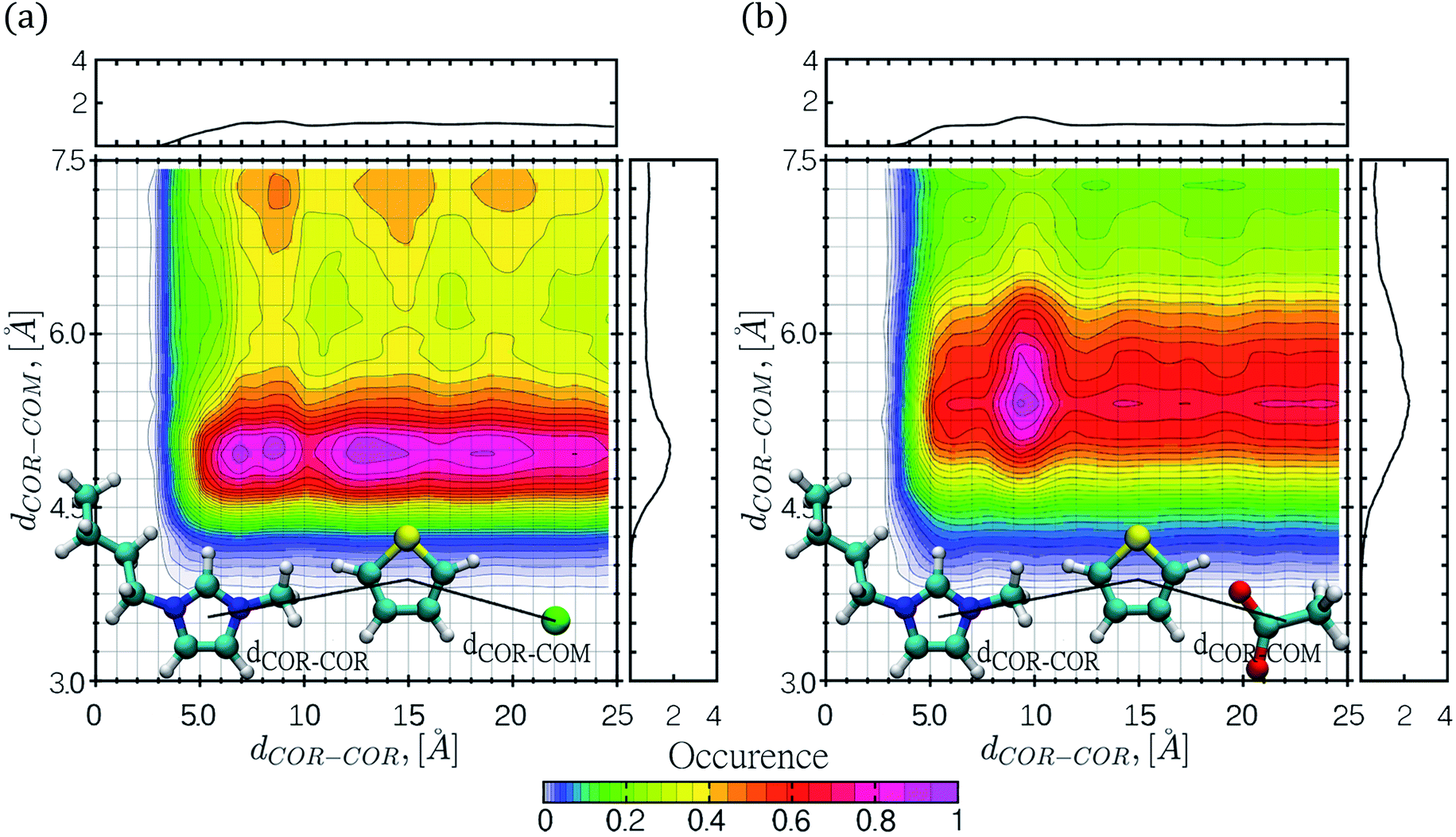

Fig. 5 Combined distribution functions (CDFs) for two distances, the first distance involves thiophene–cation interactions and the second distance comprises thiophene–anion interactions (a) thiophene in [C₄mim][Cl] IL and (b) thiophene in the [C₄mim][CH₃COO] IL. The corresponding RDFs are also displayed at the top and right side of each figure. The number of occurrences was normalized.

Fig. 6 Combined distribution functions (CDF) for the center-of-ring (COR) angle θ and distance d between thiophene and the IL cations for (a) [C₄mim][Cl] IL and (b) [C₄mim][CH₃COO] IL. The number of occurrences was normalized.

The CDF displayed in Fig. 5 corresponds to the combination of two distances, the first distance between the thiophene center-of-ring (COR) and the cation COR (d_COR–COR) and the second distance (d_COR–COM) involving the thiophene COR and the anion center-of-mass. In general, the interactions of thiophene with the IL anions frequently occurs within a narrow range of distances, while the interaction of thiophene with the IL cation occurs within a wide range of distances; in the thiophene–[C₄mim][Cl] system, the largest number of interaction occurrences are found within circular regions at d_COR–COR distances spanning from 6 to 20 Å as seen in Fig. 5a. For the [C₄mim][Br] IL, the larger interaction occurrences are located at 5.1 Å for d_COR–COR, and 4.9 Å for the d_COR–COM distance, as shown in Fig. S9b.†

Interestingly, in both CDFs corresponding to thiophene–[C₄mim][CH₃COO] and thiophene–[C₄mim][BF₄] systems, the thiophene–anion interaction comprised high occurrences within a range of 5 to 6.0 Å, as seen in Fig. 5b and S9a.†

The CDFs displayed in Fig. 6 and S10,† correspond to the thiophene–IL cation centers-of-rings (COR) distances in conjunction with the angle formed between the normal vector of the thiophene ring plane and the COR–COR distance. As observed, the COR–COR average distance occurred within a 3.4–5 Å distance range. The preferred angles are closer to 0° and 180°, suggestive of face-to-face or offset π-stacking interactions between the thiophene molecule and the imidazolium ring, in agreement with studies by Oliveira et al.²⁴ for the thiophene–[C₄mim][BF₄] system. In addition, the thiophene–[C₄mim][CH₃COO] system displayed two high interaction occurrence regions at angles close to 0° and close to 180°, within a distance of 6 Å.

The CDFs corresponding to the [Cl]⁻, [BF₄]⁻ and [Br]⁻ anions, presented high COR–COR angle distribution occurrence at the edges of 0° and 180° within 3.4 to 4.5 Å distances, as observed in Fig. 6a and S10.† Nevertheless, CDFs for the [C₄mim][CH₃COO] IL, displayed additional higher thiophene–cation interaction occurrences in the range of 45–135° within 6–7.5 Å, sampling a larger conformational space, also including edge-to-face π-stacking interactions between rings.

To further study the formation of HBs between thiophene and ILs, two additional CDFs were calculated involving two distances; the first CDF monitors the interactions between hydrogen atoms within the thiophene molecule (H_TIO) paired with negative atoms from the IL anions, and the second CDF corresponds to interactions between the sulfur atom (S_TIO) paired with hydrogen atoms from the IL cation (H₁, H₂, and H₃). These CDFs are displayed in Fig. S11 till S14 in the ESI section.†

It can be observed from Fig. S11a,† that the interactions involving H_1TIO,2TIO–Cl, and H_3TIO,4TIO–Cl atoms are concentrated in five small regions with high number of occurrences that span from 2.7 Å to 7.2 Å in both axis directions. In contrast, for the same [C₄mim][Cl] IL, the S_TIO–H_1,2,3 interactions with high occurrence are concentrated in a single region with coordinates (4.6 Å, 4.2 Å) as seen in Fig. S12a.† For the thiophene–[C₄mim][CH₃COO] system shown in Fig. S11b,† it was observed that hydrogen atoms within thiophene interacted with the oxygen atoms from the IL anion spanning a high occurrence wide-region from 2.4 Å to 7.2 Å along both axis directions. The S_TIO–H_1,2,3 interactions, presented a high number of occurrences in a region centered at coordinates (3.2 Å, 6.7 Å), as displayed in Fig. S12b.†

The CDF for the thiophene–[C₄mim][BF₄] system shown in Fig. S13a,† is very similar to the CDF displayed by the [C₄mim][CH₃COO] IL in Fig. S11a;† besides, the S_TIO–H_1,2,3 interactions presented high occurrence regions, centered at (2.9 Å, 6.5 Å) as shown in Fig. S14a.† Finally, for the thiophene–[C₄mim][Br] system, the interactions involving the H_TIO hydrogen atoms and [Br]⁻ anion (Fig. S13b†) appeared within five concentrated regions that span from 2.8 Å to 7.2 Å in both axis directions, in similitude with the CDF displayed for the thiophene–[C₄mim][Cl] system. Concerning the S_TIO–H_1,2,3 interactions, a region with high occurrences centered at (2.9 Å, 6.5 Å) was observed in Fig. S14b.†

Interaction energies

The interaction energies (E_nb) between the thiophene molecules and ILs ions were also calculated from classical MD simulations and displayed in Fig. 7. The strongest interaction in magnitude occurred between the thiophene molecule and the IL cations, with the largest negative value of −9.83 kcal mol⁻¹ corresponding to the [C₄mim][Cl] IL and a value of −9.58 kcal mol⁻¹ for the [C₄mim][Br] IL, as seen in Fig. 7a. On the other hand, the interaction energies between the thiophene molecule and the IL anion displayed the following trend in magnitude: [C₄mim][Cl] < [C₄mim][Br] < [C₄mim][BF₄] < [C₄mim][CH₃COO]. Interestingly, the strongest thiophene–anion interactions corresponded to the IL with the most favorable excess chemical potential ([C₄mim][CH₃COO]), while the strongest thiophene–cation interactions corresponded to the IL with the most unfavorable chemical potential ([C₄mim][Br]).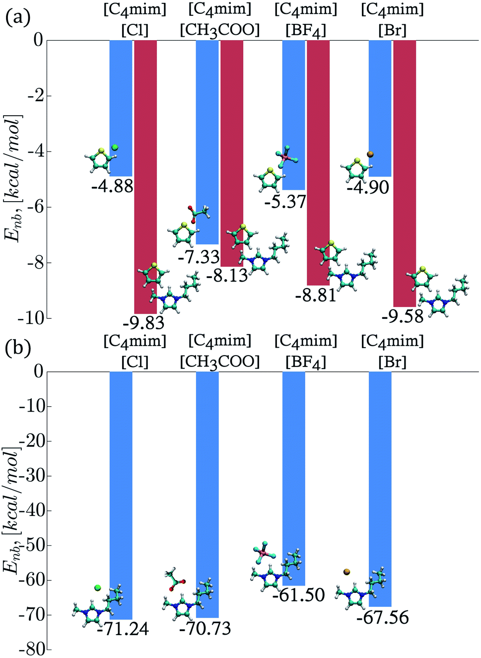

Fig. 7 Interaction energies, (a) thiophene–cation interactions are displayed in red color and the thiophene–anion interactions are displayed in blue color, (b) cation–anion interactions are shown in blue color.

Interactions energies between IL ions were also calculated, and the smallest value in magnitude corresponded to the [C₄mim][BF₄] and [C₄mim][Br] ILs as observed in Fig. 7b.

Averaged noncovalent interactions (aNCI)

The calculated aNCI for thiophene–[C₄mim][Cl] and thiophene–[C₄mim][CH₃COO] systems by means of AIMD simulations are displayed in Fig. 8; the aNCI analysis for the other two ILs can be found in the ESI† section.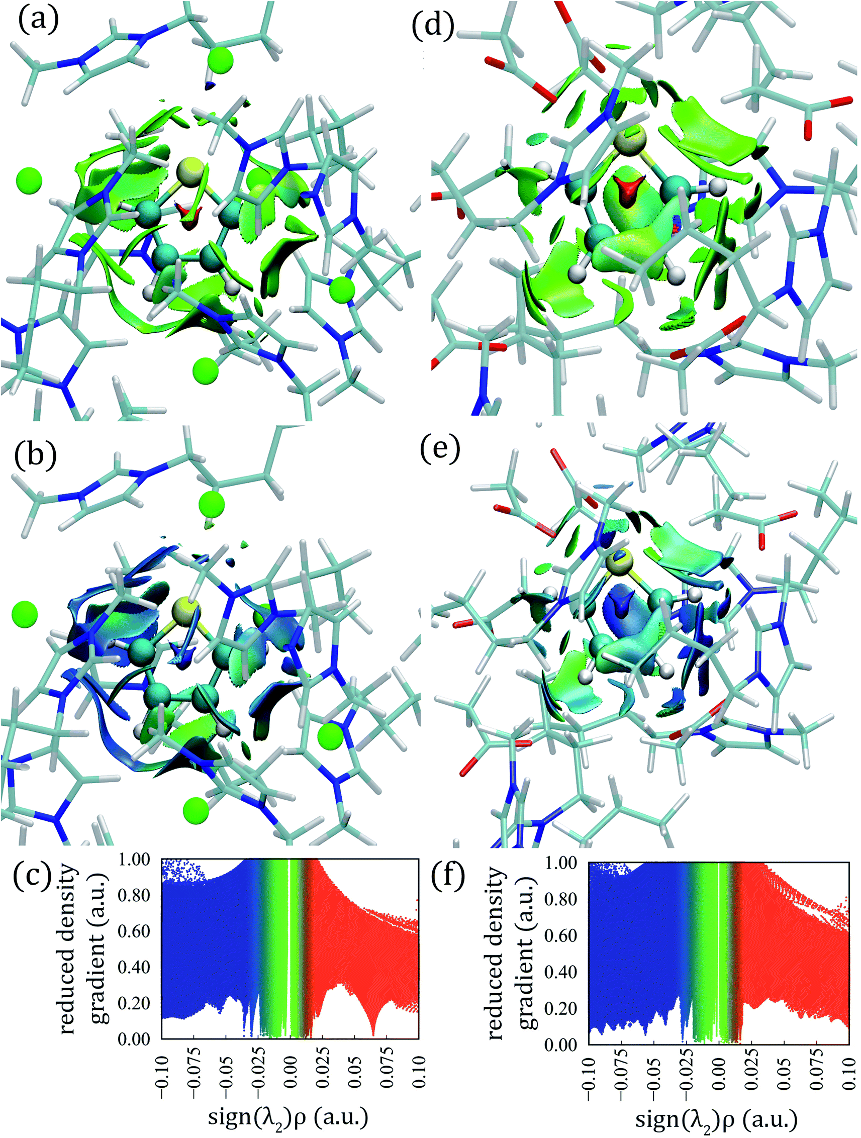

Fig. 8 Averaged noncovalent interactions between the thiophene molecule and ILs, (a) aNCI surface, (b) TFI index, and (c) reduced electronic density gradient (s) vs. density plot in the thiophene–[C₄mim][Cl] system; (d) aNCI surface, (e) TFI index and (f) reduced electronic density gradient (s) vs. density plot in the thiophene–[C₄mim][CH₃COO] system. The aNCI iso-surfaces correspond to s = 0.4 a.u., and are colored on a BGR scale of −0.04 < ρ < 0.04 a.u.; TFI iso-surfaces are colored on a BGR scale within the 0 to 1.5 range.

Large green iso-surfaces were observed in all ILs, corresponding to vdW and hydrogen bond interactions with electronic densities in the 0.0 to 0.04 a.u. range, as displayed in Fig. 8a, d, S15a, and S15d.†

The thermal fluctuation index (TFI) was also calculated, defined as the ratio between the standard deviation of the electron density and the averaged electronic density.⁸⁹ This index, monitors the stability of the noncovalent interactions within the AIMD simulations, displayed in Fig. 8b, e, S15b, and S15e;† small fluctuation values correspond to stable interactions (blue color) slightly affected by the thermal motion, while larger fluctuation values are associated with unstable interactions (red color), and green surfaces correspond to intermediate fluctuation values. All systems presented stable interactions between IL ions and thiophene, represented as blue and green TFI surfaces.

Large aNCI green surfaces surrounded the thiophene atoms within the [C₄mim][Cl] IL, while HBs appeared with electronic densities in the range 0.005 to 0.04 a.u. as seen in Fig. 8a and c. The HB between the Cl–H_TIO atoms appeared at the bottom of the thiophene molecule, the [Cl]⁻ anion fluctuated between two different H_TIO atoms giving rise to an extended green aNCI surface and extended TFI surface (Fig. 8a and b); also, a large green aNCI surface parallel to the ring plane situated at the left of the thiophene molecule appeared, corresponding to a π-stacking interaction.

For the thiophene–[C₄mim][CH₃COO] system, small circular aNCI surfaces were present around the H_TIO atoms with electronic density values between 0.005 and 0.03 a.u. as seen in Fig. 8d and f. Additionally, a green aNCI surface parallel to the thiophene ring was observed (π interaction).

Hydrogen bonds involving H_TIO–Br atoms with electronic densities in the 0.005 to 0.025 a.u. range, appeared in the [C₄mim][Br] IL; these HBs are weaker than those found in the other ILs systems, seen in Fig. S15d–f;† additionally, a vdW surface parallel to the thiophene ring was observed. Finally, within the [C₄mim][BF₄] IL, due to the tetrahedral arrangement of the four fluorine atoms, the [BF₄]⁻ anion can form two HBs with the same H_TIO atom; therefore, two circular aNCI surfaces close to each other were present; also a vdW surface parallel to the thiophene ring, corresponding to a thiophene–butyl interaction was observed in Fig. S15a–c.†

5. Conclusions

In this work, excess chemical potentials for thiophene in four imidazolium-based ionic liquids were calculated using classical molecular dynamics simulations at two temperatures, 300 K and 343.15 K. The μ^E,∞_i at 300 K and 343.15 K within these ILs showed the following trend in terms of the thiophene extraction capacity: [C₄mim][CH₃COO] > [C₄mim][BF₄] > [C₄mim][Br] > [C₄mim][Cl]. The strongest energetic interactions between the thiophene molecule and the ionic liquid anion, in combination with the weakest energetic interactions between the thiophene molecule and the ionic liquid cation, were found in ILs presenting the most favorable excess chemical potentials.

The RDFs determined at 300 K employing MD and AIMD simulations showed that the thiophene molecule interacts with the IL anions at smaller distances compared with the IL cation. The RDFs analysis for the classical MD trajectories at 343.15 K, revealed that both the location of the S_TIO–H_1,2,3, S_TIO–H_10–15 peaks and the H_TIO–anion interactions are conserved, with lower intensity values.

The AIMD simulations revealed the formation of HBs involving hydrogen atoms within the thiophene molecule paired with atoms from the IL anion, displayed as small circular aNCI surfaces with electronic densities in the 0.015 to 0.04 a.u. range.

The CDFs displayed π-stacking interactions between thiophene and the IL cation in the majority of the ILs studied; these combined distributions for the [C₄mim][BF₄], [C₄mim][Br] and [C₄mim][Cl] ILs showed both the thiophene ring and the imidazolium ring in parallel conformations at distances of 3.4 to 4.5 Å (face-to-face or offset π-stacking). In contrast, with the [C₄mim][CH₃COO] IL where the π-stacking interactions appeared at larger distances of 4.5 to 6 Å and presented more conformations, including interactions involving the thiophene ring and the butyl chain from the IL cation.

The aNCI analysis showed large green iso-surfaces corresponding primarily to vdW-type interactions between the thiophene molecule and ILs, as well as some weak to medium strength hydrogen bonds between the thiophene molecule and the IL ions.

Conflicts of interest

There are no conflicts to declare.

Acknowledgements

The authors thankfully acknowledge computer resources, technical advice, and support provided by “Laboratorio Nacional de Supercómputo del Sureste de México (LNS)”, a member of the CONACYT national laboratories. M. G. also acknowledges the high-performance computational resources provided by ACARUS at the University of Sonora. M. V. V-S. acknowledges a postdoctoral fellowship from CONACyT.

References

1. G. D. Thurston, in International Encyclopedia of Public Health ed. S. R. Quah, Academic Press, Oxford, 2nd edn, 2017, pp. 367–377.
2. H. Cai, Y.-f. Liu, J.-k. Gong, J.-q. E, Y.-h. Geng and L.-p. Yu, J. Cent. South Univ., 2014, 21, 4091–4096.
3. J. G. Speight, in Oil and Gas Corrosion Prevention. From Surface Facilities to Refineries, ed. J. G. Speight, Gulf Professional Publishing, Boston, 2014, pp. e1-e24.
4. R. Martínez-Palou and R. Luque, Energy Environ. Sci., 2014, 7, 2414–2447.
5. E. M. Broderick, M. Serban, B. Mezza and A. Bhattacharyya, ACS Sustainable Chem. Eng., 2017, 5, 3681–3684.
6. I. V. Babich and J. A. Moulijn, Fuel, 2003, 82, 607–631.
7. H. Li, L. He, J. Lu, W. Zhu, X. Jiang, Y. Wang and Y. Yan, Energy Fuels, 2009, 23, 1354–1357.
8. C. Chiappe and C. S. Pomelli, Top. Curr. Chem., 2017, 375, 52.
9. K. Kȩdra-Królik, M. Fabrice and J. N. Jaubert, Ind. Eng. Chem. Res., 2011, 50, 2296–2306.
10. E. J. Maginn, J. Phys.: Condens. Matter, 2009, 21, 373101.
11. S. Zhang, X. Lu, Q. Zhou, X. Li, X. Zhang and S. Li, in Ionic Liquids: Physicochemical Properties, ed. S. Zhang, X. Lu, Q. Zhou, X. Li, X. Zhang and S. Li, Elsevier, Amsterdam, 2009, pp. 3–20.
12. T. I. Morrow and E. J. Maginn, J. Phys. Chem. B, 2002, 106, 12807–12813.
13. Z. Lei, C. Dai and B. Chen, Chem. Rev., 2014, 114, 1289–1326.
14. W. Zheng, D. Wu, X. Feng, J. Hu, F. Zhang, Y. T. Wu and X. B. Hu, J. Mol. Liq., 2018, 263, 209–217.
15. M. Shokouhi, M. Adibi, A. H. Jalili, M. Hosseini-Jenab and A. Mehdizadeh, J. Chem. Eng. Data, 2010, 55, 1663–1668.
16. A. H. Jalili, M. Shokouhi, G. Maurer, A. T. Zoghi, J. Sadeghzah Ahari and K. Forsat, J. Chem. Thermodyn., 2019, 131, 544–556.
17. X. Wang, M. Han, H. Wan, C. Yang and G. Guan, Front. Chem. Sci. Eng., 2011, 5, 107–112.
18. M. H. Ibrahim, M. Hayyan, M. A. Hashim and A. Hayyan, Renew. Sustain. Energy Rev., 2017, 76, 1534–1549.
19. F. Rabhi, C. Hussard, H. Sifaoui and F. Mutelet, J. Mol. Liq., 2019, 289, 111169.
20. U. Domańska, M. Wlazło and M. Karpińska, Fluid Phase Equilib., 2020, 507, 112424.
21. P. Dhakal, S. N. Roese, E. M. Stalcup and A. S. Paluch, J. Chem. Eng. Data, 2018, 63, 352–364.
22. K. Paduszyński, J. Chem. Inf. Model., 2016, 56, 1420–1437.
23. J. Fang, J. Wu, C. Li, H. Li and Q. Yang, Sep. Purif. Technol., 2020, 245, 116882.
24. O. V. Oliveira, A. S. Paluch and L. T. Costa, Fuel, 2016, 175, 225–231.
25. A. L. Revelli, F. Mutelet and J. N. Jaubert, J. Chromatogr. A, 2009, 1216, 4775–4786.
26. J. D. Holbrey, I. López-Martin, G. Rothenberg, K. R. Seddon, G. Silvero and X. Zheng, Green Chem., 2008, 10, 87–92.
27. C. W. Cho, T. P. T. Pham, Y. C. Jeon and Y. S. Yun, Green Chem., 2008, 10, 67–72.
28. J. Weitkamp and Y. Traa, Catal. Today, 1999, 49, 193–199.
29. J. J. Raj, S. Magaret, M. Pranesh, K. C. Lethesh, W. C. Devi and M. I. A. Mutalib, J. Cleaner Prod., 2019, 213, 989–998.
30. A. B. Pereiro, J. M. M. Araújo, S. Martinho, F. Alves, S. Nunes, A. Matias, C. M. M. Duarte, L. P. N. Rebelo and I. M. Marrucho, ACS Sustainable Chem. Eng., 2013, 1, 427–439.
31. J. J. Raj, S. Magaret, M. Pranesh, K. C. Lethesh, W. C. Devi and M. I. A. Mutalib, Sep. Purif. Technol., 2018, 196, 115–123.
32. A. Klamt and F. Eckert, Fluid Phase Equilib., 2000, 172, 43–72.
33. J. R. Phifer, C. E. Cox, L. F. da Silva, G. G. Nogueira, A. K. P. Barbosa, R. T. Ley, S. M. Bozada, E. J. O'Loughlin and A. S. Paluch, Mol. Phys., 2017, 115, 1286–1300.
34. D. Bedrov, J. P. Piquemal, O. Borodin, A. D. MacKerell, B. Roux and C. Schröder, Chem. Rev., 2019, 119, 7940–7995.
35. S. Riahi and C. N. Rowley, J. Phys. Chem. B, 2014, 118, 1373–1380.
36. K. Goloviznina, J. N. Canongia Lopes, M. Costa Gomes and A. A. H. Pádua, J. Chem. Theory Comput., 2019, 15, 5858–5871.
37. J. K. Shah, in Annual Reports in Computational Chemistry, vol. 14, ed. D. A. Dixon, Elsevier, 2018, pp. 95–122.
38. C. W. Priest, J. A. Greathouse, M. K. Kinnan, P. D. Burton and S. B. Rempe, J. Chem. Phys., 2021, 154, 084503.
39. M. Thomas, I. Sancho Sanz, O. Hollóczki and B. Kirchner, Ab Initio Molecular Dynamics Simulations of Ionic Liquids, in NIC Symposium 2016, ed K. Binder, M. Müller, M. Kremer and A. Schnurpfeil, Verlag, Jülich, 2016, vol. 48, pp. 117–124.
40. A. D. Becke, Phys. Rev. A, 1988, 38, 3098–3100.
41. C. Lee, W. Yang and R. G. Parr, Phys. Rev. B, 1988, 37(2), 785–789.
42. J. VandeVondele and J. Hutter, J. Chem. Phys., 2007, 127, 114105.
43. A. Korotkevich, D. S. Firaha, A. A. H. Padua and B. Kirchner, Fluid Phase Equilib., 2017, 448, 59–68.
44. S. Ostadjoo, P. Berton, J. L. Shamshina and R. D. Rogers, Toxicol. Sci., 2018, 161, 249–265.
45. P. Griffin, S. Ramer, M. Winfough and J. Kostal, Green Chem., 2020, 22, 3626–3637.
46. Y. Chen and T. Mu, GreenChE, 2021, 2, 174–186.
47. J. Sánchez-Badillo, M. Gallo, S. Alvarado and D. Glossman-Mitnik, J. Phys. Chem. B, 2015, 119, 10727–10737.
48. A. L. Revelli, F. Mutelet, M. Turmine, R. Solimando and J. N. Jaubert, J. Chem. Eng. Data, 2009, 54, 90–101.
49. K. R. Seddon, A. Stark and M.-J. Torres, Clean Solvents: Alternative Media for Chemical Reactions and Processing, in ACS Symposium Series, ed. M. A. Abraham and L. Moens, American Chemical Society, Washington, 2002, ch. 4, vol. 819, pp. 34–49.
50. B. Banerjee, ChemistrySelect, 2017, 2, 8362–8376.
51. L. C. Player, B. Chan, M. Y. Lui, A. F. Masters and T. Maschmeyer, ACS Sustainable Chem. Eng., 2019, 7, 4087–4093.
52. B. Doherty, X. Zhong and O. Acevedo, J. Phys. Chem. B, 2018, 122, 2962–2974.
53. S. V. Sambasivarao and O. Acevedo, J. Chem. Theory Comput., 2009, 5, 1038–1050.
54. B. Doherty, X. Zhong, S. Gathiaka, B. Li and O. Acevedo, J. Chem. Theory Comput., 2017, 13, 6131–6145.
55. N. Rai and J. I. Siepmann, J. Phys. Chem. B, 2007, 111, 10790–10799.
56. C. Caleman, P. J. van Maaren, M. Hong, J. S. Hub, L. T. Costa and D. van der Spoel, J. Chem. Theory Comput., 2012, 8, 61–74.
57. C. Chipot and A. Pohorille, in Free Energy Calculations: Theory and Applications in Chemistry and Biology, ed. C. Chipot and A. Pohorille, Springer, Berlin, 2007, ch. 2, pp. 33–75.
58. C. H. Bennett, J. Comput. Phys., 1976, 22, 245–268.
59. M. J. Abraham, T. Murtola, R. Schulz, S. Páll, J. C. Smith, B. Hess and E. Lindahl, SoftwareX, 2015, 1–2, 19–25.
60. L. Martínez, R. Andrade, E. G. Birgin and J. M. Martínez, J. Comput. Chem., 2009, 30, 2157–2164.
61. T. Darden, D. York and L. Pedersen, J. Chem. Phys., 1993, 98, 10089–10092.
62. B. Hess, H. Bekker, H. J. C. Berendsen and J. G. E. M. Fraaije, J. Comput. Chem., 1997, 18, 1463–1472.
63. G. Bussi, D. Donadio and M. Parrinello, J. Chem. Phys., 2007, 126, 014101.
64. H. J. C. Berendsen, J. P. M. Postma, W. F. van Gunsteren, A. DiNola and J. R. Haak, J. Chem. Phys., 1984, 81, 3684–3690.
65. W. F. Van Gunsteren and H. J. C. Berendsen, Mol. Simul., 1988, 1, 173–185.
66. P. V. Klimovich, M. R. Shirts and D. L. Mobley, J. Comput.-Aided Mol. Des., 2015, 29, 397–411.
67. T. C. Beutler, A. E. Mark, R. C. van Schaik, P. R. Gerber and W. F. van Gunsteren, Chem. Phys. Lett., 1994, 222, 529–539.
68. M. J. Abraham, D. van der Spoel, E. Lindahl, B. Hess and the GROMACS development team, GROMACS User Manual version 2019.4, p. 2019.
69. J. A. Lemkul, Living J. Comp. Mol. Sci., 2019, 1, 5068.
70. T. T. Pham and M. R. Shirts, J. Chem. Phys., 2011, 135, 034114.
71. M. R. Shirts, D. L. Mobley and S. P. Brown, in Drug Design: Structure and Ligand-Based Approaches, ed. C. H. Reynolds, D. Ringe and K. M. Merz Jr, Cambridge University Press, Cambridge, 2010, pp. 61–86.
72. T. Steinbrecher, I. Joung and D. A. Case, J. Comput. Chem., 2011, 32, 3253–3263.
73. M. R. Shirts and J. D. Chodera, J. Chem. Phys., 2008, 129, 124105.
74. M. Brehm, M. Thomas, S. Gehrke and B. Kirchner, J. Chem. Phys., 2020, 152, 164105.
75. M. Brehm and B. Kirchner, J. Chem. Inf. Model., 2011, 51, 2007–2023.
76. I. Hassan, F. Ferraro and P. Imhof, Molecules, 2021, 26, 2148.
77. E. R. Johnson, S. Keinan, P. Mori-Sánchez, J. Contreras-García, A. J. Cohen and W. Yang, J. Am. Chem. Soc., 2010, 132, 6498–6506.
78. J. VandeVondele, M. Krack, F. Mohamed, M. Parrinello, T. Chassaing and J. Hutter, Comput. Phys. Commun., 2005, 167, 103–128.
79. T. D. Kühne, M. Iannuzzi, M. Del Ben, V. V. Rybkin, P. Seewald, F. Stein, T. Laino, R. Z. Khaliullin, O. Schütt, F. Schiffmann, D. Golze, J. Wilhelm, S. Chulkov, M. H. Bani-Hashemian, V. Weber, U. Borštnik, M. Taillefumier, A. S. Jakobovits, A. Lazzaro, H. Pabst, T. Müller, R. Schade, M. Guidon, S. Andermatt, N. Holmberg, G. K. Schenter, A. Hehn, A. Bussy, F. Belleflamme, G. Tabacchi, A. Glöβ, M. Lass, I. Bethune, C. J. Mundy, C. Plessl, M. Watkins, J. VandeVondele, M. Krack and J. Hutter, J. Chem. Phys., 2020, 152, 194103.
80. S. Nosé, Mol. Phys., 1984, 52, 255–268.
81. W. G. Hoover, Phys. Rev. A, 1985, 31, 1695–1697.
82. G. J. Martyna, D. J. Tobias and M. L. Klein, J. Chem. Phys., 1994, 101, 4177–4189.
83. M. Krack, Theor. Chem. Acc., 2005, 114, 145–152.
84. C. Hartwigsen, S. Goedecker and J. Hutter, Phys. Rev. B: Condens. Matter Mater. Phys., 1998, 58, 3641–3662.
85. S. Goedecker, M. Teter and J. Hutter, Phys. Rev. B: Condens. Matter Mater. Phys., 1996, 54, 1703–1710.
86. S. Grimme, S. Ehrlich and L. Goerigk, J. Comput. Chem., 2011, 32, 1456–1465.
87. S. Grimme, J. Antony, S. Ehrlich and H. Krieg, J. Chem. Phys., 2010, 132, 154104.
88. T. Lu and F. Chen, J. Comput. Chem., 2012, 33, 580–592.
89. P. Wu, R. Chaudret, X. Hu and W. Yang, J. Chem. Theory Comput., 2013, 9, 2226–2234.
90. M. A. R. Martins, J. A. P. Coutinho, S. P. Pinho and U. Domańska, J. Chem. Thermodyn., 2015, 91, 194–203.
91. D. Matkowska and T. Hofman, J. Mol. Liq., 2012, 165, 161–167.
92. J. Safarov, M. Geppert-Rybczyńska, I. Kul and E. Hassel, Fluid Phase Equilib., 2014, 383, 144–155.
93. J. Klomfar, M. Součková and J. Pátek, J. Chem. Thermodyn., 2018, 118, 225–234.
94. G. Waddington, J. W. Knowlton, D. W. Scott, G. D. Oliver, S. S. Todd, W. N. Hubbard, J. C. Smith and H. M. Huffman, J. Am. Chem. Soc., 1949, 71, 797–808.
95. W. Humphrey, A. Dalke and K. Schulten, J. Mol. Graphics, 1996, 14, 33–38.

---

Footnote

† Electronic supplementary information (ESI) available. See DOI: 10.1039/d1ra04615b

---