Typical antibiotics in the receiving rivers of direct-discharge sources of sewage across Shanghai: occurrence and source analysis

Abstract

In Shanghai, the antibiotics in the receiving rivers of direct-discharge sources of sewage (aquaculture farms, cattle farms and wastewater treatment plants) were investigated. Water and sediment samples from the receiving rivers of these sources were collected, and were screened for 19 typical antibiotics. The concentration of the antibiotics in the water and sediment ranged from not detected (ND) to 530.05 ng L⁻¹ and ND to 1039.53 ng g⁻¹, respectively, and sulfonamides and fluoroquinolones were identified as the main antibiotics in the water and sediment, respectively. According to principal component analysis with multiple linear regression (PCA-MLR), source contributions were estimated: wastewater treatment plants (66.8%) > aquaculture farms and cattle farms (21.2%), indicating that the contribution of human antibiotics was higher than veterinary antibiotics. Based on the risk quotients, ciprofloxacin was identified as the main antibiotic that causes medium risk in the aquatic ecosystem. This work systematically reflected the profile and source apportionment of antibiotics in Shanghai, which is helpful for antibiotic contamination control and environmental management.

---

1. Introduction

Antibiotics are effective in treating and preventing bacterial infection and promoting the growth of animals, and are widely used in humans and animals. However, owing to the heavy use and even abuse of antibiotics, the occurrence and potential risks of antibiotic residues in the environment are getting worse, and are the focus of attention worldwide.^1,2 Over recent years, antibiotic residues have been frequently detected in different matrices (e.g. water, sediments, soil and biological samples), among which water and sediments are the main receptors.³ The detected concentrations of antibiotics in various environmental media are in the ng–μg level.^2,4 Although the residues of antibiotics in the environment are in trace amounts, long-term and continuous exposure shows a potential risk to the ecosystem and human health.⁵ For example, Anna et al.⁶ found that sulfonamides are highly phytotoxic to duckweed, with an EC₅₀ of 0.02–4.89 mg L⁻¹. Besides, antibiotic resistant bacteria (ARB) and antibiotic resistance genes (ARG), a global health crisis, are widespread in the global environment, caused by the abuse of antibiotics.^7,8

Shanghai is one of the most developed and urbanized cities in China, with a population of up to 25 million. The volume of disposed wastewater amounts to 2.66 billion tons per year. Aquaculture and animal husbandry are relatively developed, with their output value reaching 4.83 billion yuan and 3.07 billion yuan, respectively.⁹ The river system in Shanghai is complex, with a river network density of 4.17 km km⁻². Numerous inputs of antibiotics from potential sources of pollution discharged into nearby rivers. In previous studies, multiple antibiotics were detected in the Huangpu River, which is the most important waterway in Shanghai.^10–12 Besides, these studies suggested that animal farming sites were the main polluting sources into the river,^10,11 and antibiotics could not be completely eliminated in WWTPs.¹² The elimination efficiency of antibiotics through the existing wastewater treatment process is incomplete, or even negative.^12,13

The release of antibiotics into the environment have different channels such as medical waste,¹⁴ wastewater from concentrated animal feeding operation¹⁵ and industrial and agriculture fields.¹⁶ In Shanghai, domestic and industrial wastewater enters the municipal pipeline. Aquaculture tailwater is directly discharged into surface rivers, and wastewater from livestock and poultry farms is discharged into water environment after simply treatment such as lagoons and sedimentation tanks. Therefore, wastewater treatment plants (WWTPs), livestock and poultry farms and aquafarms are the primary sources of wastewater entering the environment. For human antibiotics, WWTPs are the main sources. Aquaculture and animal husbandry are potential pollution sources of veterinary antibiotics.^17,18 In Shanghai, there is no comprehensive regional study conducted on the relative antibiotic contributions from direct-discharge sources of sewage (WWTPs, livestock and poultry farms and aquafarms). Therefore, comprehending the occurrence of antibiotics in different pollution sources in Shanghai is completely necessary.

The major objectives of present study were: (1) to determine the concentrations of typical antibiotics in surface water and sediments of the receiving rivers of WWTPs, cattle farms, and aquaculture farms in Shanghai; (2) to evaluate ecological risk of target antibiotics based on risk quotient, and (3) to estimate the contribution of the target antibiotics from the rivers near the four types of pollution sources based on principal component analysis-multiple linear regression (PCA-MLR) model, and compare the impact of veterinary antibiotics and human medical antibiotics on the surrounding natural water environment. This study can provide information for pollution regulation and source control of antibiotic in Shanghai.

2. Materials and methods

2.1 Chemicals and reagents

Nineteen target antibiotics were selected for analysis, included 9 sulfonamides (SAs): sulfadiazine (SDZ), sulfamerazine (SMR), sulfamethazine (SMZ), sulfamethoxazole (SMX), sulfathiazole (STZ), sulfapyridine (SPD), sulfamethoxydiazine (SMT), sulfisoxazole (SIA), and trimethoprim (TMP; commonly used to be a synergist with SMX¹⁹); 5 fluoroquinolones (FQs): norfloxacin (NOR), ciprofloxacin (CIP), enrofloxacin (ENR), ofloxacin (OFL), and sarafloxacin (SAR); 3 macrolides (MLs): erythromycin–H₂O (ETM–H₂O, a major degradation product of erythromycin), clarithromycin (CLR) and roxithromycin (ROX); 2 chloramphenicols (CAPs): florfenicol (FF) and chloramphenicol (CAP). All the antibiotic standards were purchased from A Chemtek Inc. (Tianjin). Erythromycin–H₂O (ETM–H₂O) was the major degradation of erythromycin and prepared by previous method.²⁰ Detail information of these compounds is shown in ESI Table S1.† Isotope-labeled ¹³C₃-caffeine used as an alternative standard was purchased from Cerilliant (Austin, TX, USA). Methanol and formic acid (HPLC-grade) were obtained from Merck (Darmstadt, Germany). Ethylenediamine tetraacetic acid disodium salt (Na₂EDTA), citrazinic acid and sodium citrate tribasic dehydrate were acquired from J&K® (Beijing, China). Ultra-pure water was provided by a Milli-Q water purification system.

2.2 Sample collection

The sampling locations are exhibited in Fig. 1. All samples (water and sediments) were collected in November, 2020. Sites A1–A6 are aquaculture farms, sites C1 and C2 are both cattle farms and sites W1–W8 are WWTPs. Sampling points were located in the receiving rivers, approximately 500 m downstream of their discharge points. Water samples (n = 16) were collected from 0 to 50 cm below surface using a stainless-steel bucket and then packed into a 2 L amber glass bottle, which rinsed with ultrapure water and methanol in advance. The surficial sediment (n = 16) was collected from a top 5 cm layer by a stainless steel grab bucket, then wrapped in aluminum foil, and stored into sealed polyethylene bags. All samples were in triplicate, stored at 4 °C and immediately transported to the laboratory and processed within 48 h.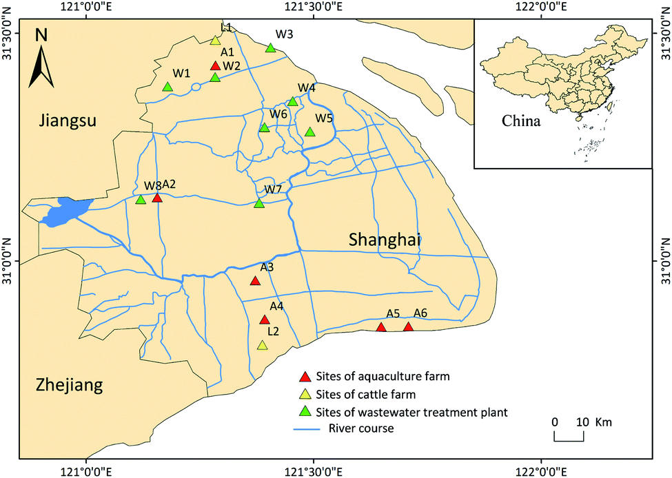

Fig. 1 Sampling sites of the receiving rivers of pollution sources in the Shanghai.

2.3 Sample preparation

The preparation and instrumental analysis of water and sediments samples were ameliorated based on previous studies.^12,21 The water samples were filtered using 110 mm neutral filter papers and 47 mm glass fiber filters (Whatman, Maidstone, England), and glass fiber filters were pre-baked in muffle for 6 hours. H₂SO₄ was added to acidify the filtrate to pH 3.0, then added 0.2 g of Na₂EDTA and stirred until complete dissolution. Before the samples passed through Oasis HLB cartridges (6 mL, 200 mg, Waters) for solid phase extraction (SPE), 100 ng ¹³C₃-caffeine was spiked into samples to monitor the recovery. The Oasis HLB cartridges were preconditioned with 6 mL methanol, 6 mL ultrapure water and 6 mL 10 mmol L⁻¹ Na₂EDTA buffer (pH 3.0). Then, the mixtures were passed through the cartridges at a flow rate of 10 mL min⁻¹. After loading, the cartridges were rinsed with 10 mL of ultrapure water (pH 3.0) and dried for 1 h. The analytes were eluted with 10 mL of methanol into 20 mL nitrogen blowpipes and evaporated to approximately 0.2 mL under nitrogen purge. Methanol was added to each tube to a final volume of 1 mL. Thereafter, the solution was filtered through a 0.22 μm organic phase needle filter (Anpel, Shanghai, China) into a 2 mL glass sample vial for analysis.

The sediment samples were all freeze-dried and ground into powder and then sieved through a 100-mesh screen. Approximately 2 g of samples (dry weight) were weighed into a 50 mL centrifuge tube. The ¹³C₃-caffeine and appropriate amounts of acetonitrile were spiked into the tubes. These tubes were vortexed on a vortex mixer and left overnight in the dark. 30 milliliters of acetonitrile solution (acetonitrile : 0.1 M EDTA–McIlvaine buffer, 50 : 50, v/v, pH = 3) was papered as extract. The extracting agent was added into centrifuge tubes and vortexed for 1 min. The samples were ultrasonic treated for 15 min at 25 °C, and then centrifuged in a centrifuge at 5000 rpm for 15 min. The extraction process was repeated 3 times. All the supernatant was mixed and transferred to a 250 mL round-bottom flask. The extract was concentrated at 50 °C via rotary evaporator, after which the residues were re-dissolved with 200 mL ultrapure water. Strong anion exchange-HLB (SAX-HLB) cartridges in tandem were used for enrichment and clean-up. The subsequent steps were repeated following the same procedures in the water sample treatment.

2.4 Instrumental analysis

High performance liquid chromatography-tandem mass spectrometry (HPLC-MS/MS) was used to monitor the target antibiotics. Chromatographic separation was performed with a UHPLC system (Waters Corp., Milford, MA) with a Phenomenex C18 reversed-phase column (100 × 3 mm, 2.6 μm). Tandem mass spectrometry was performed on a QTRAP 5500 hybrid triple quadrupole/linear ion trap mass spectrometer (AB Sciex, Ontario Canada) with a Turbo V™ ion source and ESI probe was used to achieve separate of the target compounds. The injection volume was 2 μL, the flow rate was 0.4 mL min⁻¹, and the column temperature was set at 40 °C. The mobile phase in positive ionization mode (ESI+) was ultrapure water with 0.1% (v/v) formic acid (solvent A) and 100% methanol (solvent B). In negative ionization mode (ESI−), solvent A was ultrapure water and solvent B was 100% methanol. The gradient program was as follows: 5% B held for 1 min, raised to 100% B over 5 min over 0.1 min, held for 3 min, returned to 5% B over 0.1 min, and maintained for 1 min. The MS parameters were as follows: multiple reaction monitoring (MRM) mode, capillary voltage (+): 5.5 kV, capillary voltage (−): 4.5 kV, nebuliser pressure: 45 psi, source gas temperature: 400 °C, drying gas temperature: 400 °C, source gas flow: 10 L min⁻¹ and drying gas flow: 5 L min⁻¹. Detailed optimization parameters about target compounds are shown in Table S2.†

2.5 Quality assessment and quality control (QA/QC)

Using external standard method to quantitatively target antibiotics, due to the low commercial availability of corresponding internal standards for each analyte. We used ¹³C₃-caffeine as the surrogate standard to all samples prior to enrichment to avoid possible losses during the analytical procedure, and added a blank control for every five samples. Seven standard solution concentrations (1, 2, 5, 10, 20, 50, 100 μg L⁻¹) were used to calculate the calibration curves (R² > 0.99). The method detection limits (MDLs) and the method quantitative limits (MQLs) were defined as the sample concentrations at signal-to-noise ratio (S/N) of 3 and S/N of 10, respectively. The MDLs of the water and sediment samples ranged from 0.53 ng L⁻¹ to 10.13 ng L⁻¹ and from 0.01 ng g⁻¹ to 0.81 ng g⁻¹, respectively. The recoveries of water and sediment samples ranged from 67% to 96% and 57% to 92%, respectively. The details are shown in Table S3.†

2.6 Environmental risk assessment

The antibiotic ecotoxicological risk assessment is usually based on the European Medicines Agency (EMA), in which risk quotient (RQ) is calculated as ratio between the measured environmental concentration (MEC) and the predicted no-effect concentration (PNEC),²² as exhibited in eqn (1) and (2):

RQ = MEC/PNEC_wat (1)

PNEC_wat = (L(E)C₅₀)/AF or PNEC_wat = NOEC/AF (2)

where the L(E)C₅₀ represent acute toxicity, and NOEC represent chronic toxicity. The assessment factor (AF) shows whether the toxicity is acute (1000) or chronic (100).²³ Generally speaking, NOEC is preferred according to European technical guidance document. The toxicity data for the most sensitive organism are obtained according to the ECOSAR model or published literature (Table S3†). For interpretation, RQs were classified into four levels: RQ < 0.01 indicates insignificant risk; 0.01 < RQ < 0.1 a low risk; 0.1 < RQ < 1.0 a medium risk; RQ > 1.0 a high risk.²⁴

Due to the lack toxicities of antibiotics in soils, few studies reported the risk of antibiotics in the sediments. The value of PNEC in the sediments (PNEC_sed) was estimated from PNEC_wat values through the soil–water equilibrium partitioning approach as the following equation:²⁵

PNEC_sed = PNEC_wat × K_sed (3)

where K_sed is the partition coefficient of compound between sediment and water.

2.7 PCA-MLR model

The source contribution analysis was conducted using the PCA-MLR mode,²⁶ which was calculated according to the following formula:

Ĉ_sum = ∑B_kFS_k (4)

Ĉ_sum = (C_sum − mean[C_sum]/σ) (5)

where Ĉ_sum is the standard normalized deviation of the sum of the antibiotic concentrations, σ is the standard deviation of the antibiotics concentration, B_k is the regression coefficient, and FS_k is the factor score calculated by the PCA analysis.

The equation of the mean percentage contribution of each source (factor) is calculated by B_k/∑B_k, and the contribution of each source k is as follows:

Contribution of source k (ng L⁻¹) = mean[C_sum] × (B_k/∑B_k) + B_kσFS_k (6)

2.8 Statistical analysis

Data was analyzed by IBM SPSS Statistics 21. If the P value <0.05, analysis was considered to be significant. The figures were made by Origin 9.0, ArcMap 10.4.1 and Heml 1.0.

3. Results and discussion

3.1 Occurrence of antibiotics in surface water

The occurrence and concentration of target antibiotics in all water samples were presented in Table 1. Among the nineteen antibiotics from four classes, two antibiotics (ENR and CAP) were not detected, while other antibiotics had high detection rate above 60% except NOR (25%), SAR (25%), ETM–H₂O (18.8%) and CLR (25%). The mean concentration ranged from not detected (ND) to 80.88 ng L⁻¹ (SPD), and the maximum concentration was 530.50 ng L⁻¹ (SPD).

Table 1 The concentrations of the target antibiotics in water samples and sediment samples

	SAs									FQs					MLs			CAPs
	SDZ	SMR	SMZ	SMX	STZ	SPD	SMT	SIA	TMP	NOR	CIP	ENR	OFL	SAR	ETM–H2O	CLR	ROX	FF	CAP
a Not detected.
Water samples (ng L^−1)
Freq (%)	87.5	100.0	100.0	100.0	100.0	93.8	93.8	93.8	81.3	25.0	62.5	0.0	75.0	25	18.8	25.0	56.3	100.0	0.0
Mean	17.89	40.38	68.14	21.05	17.64	80.88	15.80	6.44	6.26	13.05	20.46	ND	25.12	1.68	ND	3.76	2.27	3.96	ND
Max	76.75	140.20	331.50	35.14	47.51	530.05	39.80	15.63	9.86	26.74	35.68	ND	40.02	5.85	7.25	10.05	7.09	11.58	ND
Min	ND^a	7.26	10.86	8.83	2.42	ND	ND	ND	ND	ND	ND	ND	ND	ND	ND	ND	ND	3.44	ND
Sediment samples (ng g^−1)
Freq (%)	81.5	93.8	81.3	18.8	18.8	100.0	18.8	37.5	62.5	68.8	56.3	25.0	100.0	0.0	87.5	75.0	93.8	6.3	0.0
Mean	0.69	2.14	0.28	0.06	0.17	2.90	0.04	0.37	0.35	5.21	16.07	0.43	102.98	ND	0.40	0.72	0.54	ND	ND
Max	2.21	7.98	0.92	0.63	2.69	18.46	0.47	3.13	4.13	32.34	64.58	3.46	1039.53	ND	2.02	4.14	3.31	0.09	ND
Min	ND	ND	ND	ND	ND	0.23	ND	ND	ND	ND	ND	ND	0.19	ND	ND	ND	ND	ND	ND

---

Relatively, all SAs had higher detection frequency (>80%). The total concentration of SPD was the highest (ND to 530.50 ng L⁻¹), with detection frequency of 93.8%. Compound SMR and SMZ were also predominant antibiotics, with total concentrations ranged from 7.26 ng L⁻¹ to 142.20 ng L⁻¹ and 10.86 ng L⁻¹ to 331.50 ng L⁻¹, respectively. The occurrence of high concentrations of SMR and SPD was similar to previous study of the surface water of Shanghai,³⁹ which may be attributed to the extensive use of these chemicals. Previous study indicated that sulfonamides have a good activity of water-solubility with weakly adsorption to sediments or sludge, which was also a reason for their high concentration and detection frequencies in the surface waters.⁴⁰ In the groups of FQs, CIP and OFL were predominant antibiotics. Relative to low detected for NOR and ENR, CIP and OFL were detected ranged from ND to 35.68 ng L⁻¹ and ND to 40.02 ng L⁻¹, respectively, with detection frequencies of 62.5% and 75.0%, respectively. It is because CIP and OFL are more stable and have longer half-life.^41,42 Duong et al. indicated that FQs are easily photodegraded and adsorbed by sediments.⁴³ Regarding MLs, ROX was the predominant antibiotics, with total concentration of ND to 7.09 ng L⁻¹. The detection frequency of ROX was the highest (56.3%), but the maximum concentration was CLR (10.05 ng L⁻¹). The low concentrations of MLs was similar to related studies,^39,44 which was attributed that MLs might be photodegraded under the action of organic carbon as photosensitizer in natural water.⁴⁵ Zero detected for the antibiotic CAP can be attributed to the prohibition of CAP in China since 2002, which is similar to previous study.³⁹ The phase-out of CAP led to the increasing use of FF, which was the substitute of CAP. FF was detected at all sample sites and the average concentration reached 4.98 ng L⁻¹. This result was consistent with previous study in Huangpu River,¹¹ but the average concentration of FF (116.3 ng L⁻¹) in previous study was much higher than those in present study, which could indicate a decrease in the use of FF in Shanghai.

The concentrations of antibiotics for receiving water body near the three source types (aquaculture farm, cattle farm and WWTP) are shown in Fig. 2(A). This figure contains thirteen antibiotics (SDZ, SMR, SMZ, SMX, STZ, SPD, SIA, TMP, CIP, OFL, ROX and FF) and other six compounds (NOR, ENR, SAR, ETM–H₂O and CAP) are excluded due to their lower detection frequencies (<30%). In the group of aquaculture farm, SMR and SMZ were the predominant antibiotics, and the highest concentration of SMZ reached 145.46 ng L⁻¹. SMZ was aquaculture approved antibiotic in China [http://www.fishfirst.cn/article-35467-1.html], which lead to relatively high residues in present study. As a human antibiotic, SMR in such high concentration maybe due to the discharge of other pollution sources. Occurrence of SMZ and SMR is 1–2 order of magnitude higher than those in upper Huangpu River in Shanghai,⁴⁶ which can be attributed to the attenuation in stream. Although massive consumption in aquaculture, the detection frequency of FQs was low (33.3%) in this study, which can be attributed to the relatively fast rate of photodegradation. In the group of cattle farm, FQs, MLs and CAPs were not detected except for FF. Specifically, eight SAs were 100% discovered and the concentration of SMX was relatively higher. In the group of WWTP, almost all SAs could be detected for their stability in water, of which high concentrations of SPD with a peak concentration of 530.05 ng L⁻¹ were detected in W1. FQs had the detection rate of 54.16% at the eight sampling sites. Among them, OFL and CIP was obvious higher with the highest concentration of 40.02 ng L⁻¹ and 35.68 ng L⁻¹, respectively. OFL and CIP were widely used human pharmaceutical. In a word, the concentration of antibiotics in the WWTPs groups was higher than those of other sources, indicating significant contribution of WWTPs to total antibiotic residues in Shanghai. In addition, this study also confirmed that cattle farms have limited contribution of antibiotics in surface water bodies in Shanghai.

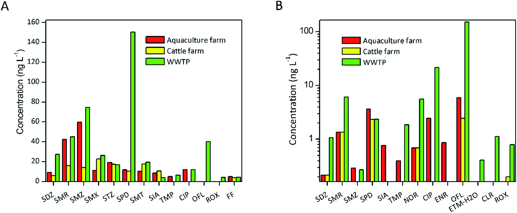Fig. 2 Compositional patterns of different antibiotics in water samples (A) and sediment samples (B) of three source types.

The status of antibiotics in water of the WWTPs and cattle farms receiving rivers were comparable with those in WWTPs and livestock and poultry farms-impacted rivers in other literatures. Since studies on the detection of antibiotics in the receiving rivers of aquaculture farms were few, the antibiotic concentrations in the receiving rivers of aquaculture farms were compared with those in the water in aquaculture farms (Table 2). In the group of WWTPs, the antibiotic levels in this study were similar to those in Kunming,²⁷ higher than those in the Ebro delta (Spain)³⁰ and lower than those in Kenyan,²⁹ Durban (South Africa)³¹ and Girona (Spain).²⁸ In the group of aquaculture farms, the concentrations of antibiotics in this study were comparable to those in Hangzhou Bay,³² Guangdong³⁴ and Bangladesh,³⁵ but higher than those in Pearl River Delta (PRD).³³ This result may be attribute to there is a mariculture in PRD and its dilution effect is relatively strong. In the group of cattle farms, the antibiotic concentrations were lower than those in Guangxi,¹⁸ Jiangsu³⁶ and Thailand,³⁸ but higher than America.³⁷ Overall, the antibiotics pollution level in Shanghai is moderate compared with other research areas at domestic and overseas.

Table 2 Global concentration comparison of main compounds in surface water (ng L⁻¹)

	SDZ	SMR	SMZ	SMX	SPD	TMP	ENR	NOR	CIP	OFL	ETM–H2O	CLR	ROX	FF	References
The group of WWTPs
Shanghai	27.45	45	74.64	26.09	150.25	6.55	ND	8.25	22.18	32.12	4.11	ND	3.02	4.35	This present study
Kunming		ND		21.3		5.8			ND			4	13.9		27
Girona (Spain)				40.2					50	100.7		61.3			28
Kenyan			750			3.5		54.5	300						29
The Ebro delta (Spain)	0.1		2	0.2	0.15	0.4			0.05	0.6		0.45	0.2		30
Durban (South Africa)				194.27				0.6	310.75	33.45		13.48	ND		31
The group of aquaculture farms
Shanghai	9.14	42.26	59.57	11.23	11.89	4.92	ND	15.08	12.19	20.56	ND	ND	ND	7.02	This present study
Hangzhou Bay	1.59		20.42	6.87			ND	55.24							32
Pearl River Delta	ND	ND	ND	0.7	ND	0.3		6.4	ND	5.5	ND	ND	ND		33
Guangdong			2.03	18.25			18.18	31.33	27.77						34
Bangladesh	1.84		1.56	6.71		8.94					ND		ND		35
The group of cattle farms
Shanghai	5.82	15.74	14.18	22.76	10.39	ND	ND	ND	ND	ND	ND	ND	ND	5.07	This present study
Guangxi	109.29		82.4	7.74				7.4	4.46	7.25				26.05	18
Jiangsu	270		100	90											36
America			ND			0.16		ND	ND	ND	ND				37
Thailand	95	0.58				58.3		2.65						7.75	38

---

3.2 Occurrence of antibiotics in sediments

The occurrence and concentration of antibiotics in sediments were summarized in Table 1. Except SAR and CAP, all target antibiotics were detected in the sedimentary phase. The mean concentration of antibiotics ranged from ND to 102.98 ng g⁻¹ (OFL), and the maximum concentration was 1039.53 ng g⁻¹ (OFL) (on a dry weight basis). Due to the stable existence state, sediments are important sink of contaminants to enrich antibiotics. Moreover, sediments are in an anaerobic environment that inhibit the degradation of antibiotics. Therefore, the concentrations of some antibiotics in sediments are greater than in water.

In comparison, FQs was predominant class of contaminants. As mentioned above, it was attribute to the strong adsorption of FQs to particles, which delay their degradation.⁵⁰ OFL had the highest concentration and detection frequency in sediments, which can be explained by the extensive use and low degradation in the environment. NOR, CIP and ENR, as widely use drugs, had high detection concentrations. However, SAR was not detected in sediments. This may be due to the reasons that SAR is an animal-specific medicine, mainly used to treat poultry colibacillosis, and there is no large-scale livestock and poultry breeding base. The compounds ETM–H₂O, CLR and ROX were at similar level, ranging from ND to 2.02 ng g⁻¹, ND to 4.14 ng g⁻¹ and ND to 3.31 ng g⁻¹, respectively. The concentrations of MLs were low, but their detection frequencies were high, 87.5% (ETM–H₂O), 75.0% (CLR) and 93.8% (ROX). Although previous study reported that MLs mainly existed in cationic form and adsorbed on particles because of high K_OW.⁵¹ The low concentrations of MLs can be attributed to limited usage in present study area. In the group of SAs, the concentrations were low due to their stronger hydrophilicity.⁵² The groups of CAPs showed the least content detection, and the antibiotic CAP were also not detected in sedimentary phase. This shows that local aquaculture farmers strictly abide by the ban of antibiotics.

Fig. 2(B) exhibits the compositional patterns of the selected antibiotics in the sediments of the receiving rivers near the four source types. According to the detection frequencies greater than 30%, thirteen antibiotics (SDZ, SMR, SMZ, SPD, SIA, TMP, NOR, CIP, ENR, OFL, ETM–H₂O, CLR and ROX) are contained. In the groups of aquaculture farm and cattle farm, the average concentrations of all the selected antibiotics were lower than 10 ng g⁻¹. Among them, OFL was the predominant antibiotic with the highest concentrations of 15.48 ng g⁻¹ and 2.77 ng g⁻¹ in two groups, respectively. OFL also was the main antibiotic in the groups of WWTP. Besides, the average levels of OFL in WWTP (151.63 ng g⁻¹) was 2 orders of magnitude larger than aquaculture farm and cattle farm (5.92 ng g⁻¹ and 2.43 ng g⁻¹). This phenomenon was different from those in water, which can be attribute to various adsorption of antibiotics. Relatively speaking, the antibiotics contribution of WWTP in sediment were higher.

Table 3 showed the comparison of antibiotic concentrations in sediments in this research and those in other literatures. The results of comparison of three sources showed that the overall concentrations of antibiotic in this study is moderate. It is worth that OFL content in sediments in the receiving river of WWTPs was at a high level. This phenomenon might be caused by its extensive use in Shanghai. Mei et al. reported that the high concentration of OFL discharge from WWTPs in Shanghai (10² to 10³ ng L⁻¹).⁵³

Table 3 Global concentration comparison of main compounds in sediment (ng g⁻¹)

	SDZ	SMR	SMZ	SMX	STZ	SPD	SIA	TMP	NOR	CIP	ENR	OFL	ETM–H2O	CLR	ROX	Reference
The group of WWTPs
Shanghai	1.07	6.06	0.27	0.07	0.40	2.36	ND	1.86	5.58	21.66	ND	151.63	0.41	1.12	0.79	This present study
Beijing	0.4			0.53						10.5		39.5			6.55	47
Kenyan				10.03				3.5	11.33	5						29
Córdoba (Argentina)					ND			ND	ND	ND		ND		ND		48
The group of aquaculture farms
Shanghai	0.22	1.35	0.29	0.07	ND	3.67	0.76	0.40	0.69	2.45	0.87	5.92	0.06	0.14	0.16	This present study
Hangzhou Bay	ND		1.37	ND					7.33		1.22					32
Pearl River Delta	ND	ND	ND	ND	ND	ND		0.2	2.2	0.2		0.4	0.04	0.2	0.2	33
Guangdong			3.91	3.25					1.15	4.07	366.75					34
The group of cattle farms
Shanghai	0.22	1.35	0.14	ND	ND	2.33	ND	ND	ND	ND	ND	ND	ND	ND	ND	This present study
Guangxi	ND		4.75	ND					23.75	14.61	79.15	126.35				18
Jianghan Plain (China)	1.5	1.6	ND	2.7	ND				47.6	17.7	16.9			0.9	2.0	49

---

3.3 Potential sources of antibiotics in Shanghai

The source contributions were further determined by principal component analysis, followed by multiple linear regression (PCA-MLR). Thirteen compounds used for PCAs are shown in Table 4 (antibiotics with low detection rate are not shown). Four principal components (PC1, PC2, PC3, and PC4) obtained after varimax rotation, which accounted for 21.64%, 15.01%, 14.74% and 12.92% of the total variance, respectively. The first rotated component (PC1) is mainly associated with five antibiotics: SDZ, SMX, SPD and SMT, which are important antibiotics used in the therapy of human. Thus, PC1 can indicate human pharmaceutical use and domestic discharge to water environment from WWTPs. The profile of the second rotated component (PC2) is characterized by high loading of three antibiotics: SMR, SMZ and FF, which are widely used in veterinary drugs. Therefore, PC2 appears to be indicative of veterinary drugs. Previous studies reported that animal farms were main pollution sources in the Huangpu River, Shanghai.^11,46 OFL is the largest loading on the third rotated component (PC3). SIA is the largest loading on PC4. These chemicals can indicate human pharmaceutical.

Table 4 Varimax-rotated component matrix of all water samples^a

Antibiotics	Component
	1	2	3	4
a Extraction method: principal component analysis; rotation method: varimax with Kaiser normalization.
SDZ	0.900	0.025	−0.077	0.088
SMR	−0.107	0.552	−0.181	−0.011
SMZ	0.131	0.814	−0.030	0.126
SMX	0.701	0.307	0.147	−0.316
STZ	0.007	−0.162	0.046	−0.249
SPD	0.783	−0.338	−0.108	−0.115
SMT	0.686	0.349	−0.239	−0.003
SIA	0.015	0.012	−0.079	0.903
TMP	0.391	0.211	−0.681	0.324
CIP	−0.031	0.430	0.115	0.307
OFL	−0.086	−0.146	0.805	0.205
ROX	0.486	−0.271	−0.343	−0.642
FF	0.047	0.731	0.450	−0.106
Percentage variance explained (%)	21.64	15.01	14.74	12.92

---

In order to confirm the mass apportionment of the four components, multiple linear regression of elements in the factor scores matrix (FS_k) against the standard normalized deviate of the sum antibiotics values (Ĉ_sum) performed on PCA score was analyzed. The equation was as follows:

Ĉ_sum = 0.813FS₁ + 0.259FS₂ + 0.145FS₃ (R² = 0.751)

The Ĉ_sum equation can be expanded as follows:

Ĉ_sum = 0.813FS₁σ + 0.259FS₂σ + 0.145FS₃σ + mean[Ĉ_sum]

where σ was 294.48 ng L⁻¹; and mean[Ĉ_sum] was 195.65 ng L⁻¹. The analysis demonstrated that the first three components (PC1, PC2, and PC3) were retained. The mean contribution B_k/∑B_k of each factor was estimated, and the WWTPs (factor 1) accounted for 66.8%. The contribution from aquaculture farms and cattle farms (factor 2) was 21.2%, and human pharmaceutical (factor 3) was 11.9%. Therefore, the contribution of human antibiotics to the aquatic environment was relatively higher than veterinary antibiotics in Shanghai.

3.4 Environmental risk assessment

Fig. 3 shows different pollution sources of ecological risks for 19 antibiotics in surface waters and sediments. In case of surface water (group a), the average RQ_total values in aquaculture farms, cattle farm and WWTP were 0.88, 0.09 and 1.42, respectively. The calculated RQ values of most antibiotics were lower than 0.1, indicating the relatively low risk in the aquatic environment. CIP and SPD were the dominant risk contributors, and the RQ value ranged from 0 to 0.71 and 0 to 1.15, respectively. To be specific, CIP showed insignificant and medium risk in 37.5% and 62.5% of all samples, respectively. SPD showed insignificant, low and medium risk in 16.7%, 16.7% and 62.5% of all samples, respectively, while only 4.17% of all samples exhibited high risk. The highest risk occurred in WWTPs, of which SPD, CIP and ETM–H₂O were the central contributors, with mean RQ values of 0.32, 0.72 and 0.21, respectively. With regard to sediment (group b), the mean RQ_total values were 0.55, 0.31 and 1.12 in aquaculture farms, cattle farm and WWTP, respectively. As was the case with surface water, higher risks were evaluated in sediments of WWTP. Besides, the calculated RQ_total values of WWTP were also higher in sediments. CIP was the main risk contributor, and the RQ values were larger than 0.1 in 58.33% samples and posed medium risk. Meanwhile ETM–H₂O and CLR also presented medium risk (>30%) in sediments. Especially, compared to SAs, FQs and MLs posed higher ecological risks to the relevant sensitive aquatic organisms. This result was consistent with the multimedia fate modelling of antibiotics in the previous study of Beijing that FQs and MLs had higher ecological risks than SAs.⁵⁴ All in all, the levels of antibiotics detected in surface water and sediments would not cause a high risk to aquatic organisms. However, long-term continuous emissions into aquatic ecosystems may lead to negative effects and thus should be vigilant. Furthermore, given the fact that interaction of various antibiotics may exert higher ecological risk,⁵⁵ further investigations are needed.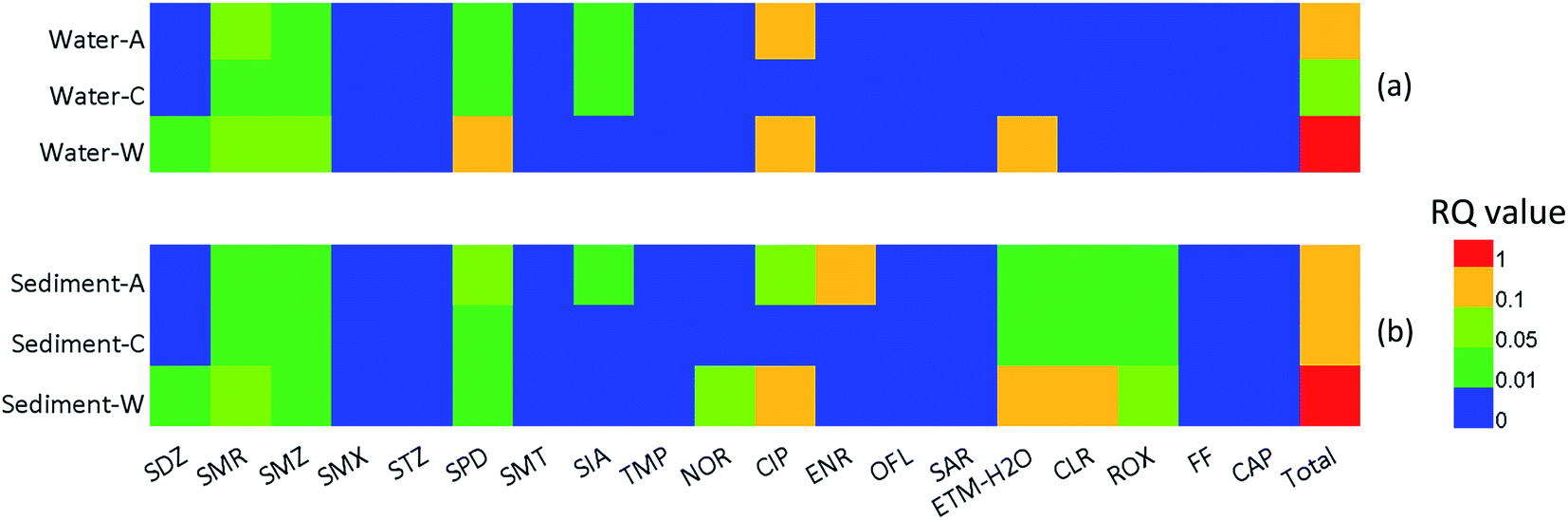

Fig. 3 Spatial ecological risk differences of 19 individual antibiotics in receiving water body of three source types (aquaculture farm, cattle farm and WWTP) (group (a) represents ecological risk variation in surface water; group (b) represents ecological risk variation in sediments).

4. Conclusion

Nineteen antibiotics were investigated in the surface water and sediment of receiving rivers near potential sources in Shanghai. The results showed that SAs and FQs were the predominant antibiotic in surface water and sediment, respectively. The pollution of human antibiotics was greater than that of veterinary antibiotics, and WWTPs should be considered as a main source of antibiotics in Shanghai. Given this situation, wastewater treatment efficiency need to be improved. Risk assessment revealed that CIP posed medium risks to aquatic ecosystem. Further study is needed to better understand the transmission mechanism of potential sources of antibiotics in Shanghai, and their impact on the public health.

Author contributions

Dong Li: conceptualization, methodology, sample collection, writing original draft preparation. Huozhu Hao: sample collection. Haiyang Shao: software, validation. Nan Xie: data curation. Jianzhong Gu: investigation, sample collection. Gang Xu: funding acquisition, supervision, writing – reviewing and editing.

Conflicts of interest

There are no conflicts to declare.

Acknowledgements

This work was financially supported by the National Natural Science Foundation of China (41773121, 11975147, 11875185, 11775138) and by National Key Research and Development Project (No. 2020YFC1808200).

Notes and references

1. Q. Bu, B. Wang, J. Huang, S. Deng and G. Yu, J. Hazard. Mater., 2013, 262, 189–211.
2. M. C. Danner, A. Robertson, V. Behrends and J. Reiss, Sci. Total Environ., 2019, 664, 793–804.
3. F. Huang, Z. An, M. J. Moran and F. Liu, J. Hazard. Mater., 2020, 399, 122813.
4. J. L. Liu and M. H. Wong, Environ. Int., 2013, 59, 208–224.
5. M. Ashfaq, K. Nawaz Khan, M. Saif Ur Rehman, G. Mustafa, M. Faizan Nazar, Q. Sun, J. Iqbal, S. I. Mulla and C.-P. Yu, Ecotoxicol. Environ. Saf., 2017, 136, 31–39.
6. A. Białk-Bielińska, S. Stolte, J. Arning, U. Uebers, A. Böschen, P. Stepnowski and M. Matzke, Chemosphere, 2011, 85, 928–933.
7. M. Qiao, G. G. Ying, A. C. Singer and Y. G. Zhu, Environ. Int., 2018, 110, 160–172.
8. J. L. Martínez, Science, 2008, 321, 365–367.
9. SONBSS and SMSB, Shanghai Municipal Statistics Bureau and Survey Office of the National Bureau of Statistics in Shanghai, China Statistics Press, Beijing, 2019.
10. L. Jiang, X. Hu, D. Yin, H. Zhang and Z. Yu, Chemosphere, 2011, 82, 822–828.
11. K. Chen and J. L. Zhou, Chemosphere, 2014, 95, 604–612.
12. M. H. Wu, C. J. Que, G. Xu, Y. F. Sun, J. Ma, H. Xu, R. Sun and L. Tang, Ecotoxicol. Environ. Saf., 2016, 132, 132–139.
13. S. Aydin, M. E. Aydin, A. Ulvi and H. Kilic, Environ. Sci. Pollut. Res., 2018, 26, 544–558.
14. A. L. Pereira, R. T. D. Barros and S. R. Pereira, Environ. Sci. Pollut. Res., 2017, 24, 24061–24075.
15. K. L. Martin, R. E. Emanuel and J. M. Vose, Sci. Total Environ., 2018, 642, 887–893.
16. J. Lee, J. H. Jeon, J. Shin, H. M. Jang, S. Kim, M. S. Song and Y. M. Kim, Sci. Total Environ., 2017, 605, 906–914.
17. X. Liu, J. C. Steele and X. Z. Meng, Environ. Pollut., 2017, 223, 161–169.
18. L.-J. Zhou, G.-G. Ying, S. Liu, R.-Q. Zhang, H.-J. Lai, Z.-F. Chen and C.-G. Pan, Sci. Total Environ., 2013, 444, 183–195.
19. M. C. Dodd and C.-H. Huang, Water Res., 2007, 41, 647–655.
20. C. S. McArdell, E. Molnar, M. J. F. Suter and W. Giger, Environ. Sci. Technol., 2003, 37, 5479–5486.
21. Y. Hu, X. Yan, Y. Shen, M. Di and J. Wang, Ecotoxicol. Environ. Saf., 2018, 157, 150–158.
22. M. Grung, T. Kallqvist, S. Sakshaug, S. Skurtveit and K. V. Thomas, Ecotoxicol. Environ. Saf., 2008, 71, 328–340.
23. H. Ding, Y. Wu, W. Zhang, J. Zhong, Q. Lou, P. Yang and Y. Fang, Chemosphere, 2017, 184, 137–147.
24. M. D. Hernando, M. Mezcua, A. R. Fernandez-Alba and D. Barcelo, Talanta, 2006, 69, 334–342.
25. X. L. Wu, L. Xiang, Q. Y. Yan, Y. N. Jiang, Y. W. Li, X. P. Huang, H. Li, Q. Y. Cai and C. H. Mo, Sci. Total Environ., 2014, 487, 399–406.
26. J. J. Jiang, C. L. Lee, P. Brimblecombe, L. Vydrova and M. D. Fang, Environ. Pollut., 2016, 208, 79–86.
27. H. Huang, S. Zeng, X. Dong, D. Li, Y. Zhang, M. He and P. Du, J. Environ. Manage., 2019, 231, 494–503.
28. S. Rodriguez-Mozaz, S. Chamorro, E. Marti, B. Huerta, M. Gros, A. Sanchez-Melsio, C. M. Borrego, D. Barcelo and J. L. Balcazar, Water Res., 2015, 69, 234–242.
29. P. Kairigo, E. Ngumba, L. R. Sundberg, A. Gachanja and T. Tuhkanen, Sci. Total Environ., 2020, 720, 137580.
30. A. Serra-Compte, M. G. Pikkemaat, A. Elferink, D. Almeida, J. Diogene, J. A. Campillo, M. Llorca, D. Alvarez-Munoz, D. Barcelo and S. Rodriguez-Mozaz, Environ. Pollut., 2021, 271, 116313.
31. A. C. Faleye, A. A. Adegoke, K. Ramluckan, J. Fick, F. Bux and T. A. Stenstrom, Sci. Total Environ., 2019, 678, 10–20.
32. J. Yuan, M. Ni, M. Liu, Y. Zheng and Z. Gu, Mar. Pollut. Bull., 2019, 138, 376–384.
33. H. Xie, H. Hao, N. Xu, X. Liang, D. Gao, Y. Xu, Y. Gao, H. Tao and M. Wong, Sci. Total Environ., 2019, 659, 230–239.
34. W. Xiong, Y. Sun, T. Zhang, X. Ding, Y. Li, M. Wang and Z. Zeng, Microb. Ecol., 2015, 70, 425–432.
35. A. Hossain, S. Nakamichi, M. Habibullah-Al-Mamun, K. Tani, S. Masunaga and H. Matsuda, Chemosphere, 2017, 188, 329–336.
36. R. Wei, F. Ge, S. Huang, M. Chen and R. Wang, Chemosphere, 2011, 82, 1408–1414.
37. E. R. Campagnolo, K. R. Johnson, A. Karpati, C. S. Rubin, D. W. Kolpin, M. T. Meyer, J. E. Esteban, R. W. Currier, K. Smith, K. M. Thu and M. McGeehin, Sci. Total Environ., 2002, 299, 89–95.
38. R. Chan, S. Wandee, M. Wang, W. Chiemchaisri, C. Chiemchaisri and C. Yoshimura, Agric., Ecosyst. Environ., 2020, 304, 107123.
39. F. Zhu, S. Wang, Y. Liu, M. Wu, H. Wang and G. Xu, Environ. Sci. Pollut. Res. Int., 2021, 28, 9836–9848.
40. Y. Luo, L. Xu, M. Rysz, Y. Q. Wang, H. Zhang and P. J. J. Alvarez, Environ. Sci. Technol., 2011, 45, 1827–1833.
41. R. Andreozzi, R. Marotta and N. Paxeus, Chemosphere, 2003, 50, 1319–1330.
42. Q. j. Ji, Residue and Degradation of Three Fluoroquinolones in Pig Manure, Anhui Agricultural University, 2012.
43. H. A. Duong, N. H. Pham, H. T. Nguyen, T. T. Hoang, H. V. Pham, V. C. Pham, M. Berg, W. Giger and A. C. Alder, Chemosphere, 2008, 72, 968–973.
44. C. Pan, Y. Bao and B. Xu, Chemosphere, 2020, 239, 124816.
45. T.-H. Yu, A. Y.-C. Lin, S. K. Lateef, C.-F. Lin and P.-Y. Yang, Chemosphere, 2009, 77, 175–181.
46. W. Q. Fang Longfei, W. Yuanhong, Y. Lanlan, L. Zongchan and L. Jianshe, Environ. Pollut. Control, 2017, 39, 301–306.
47. X. Guo, C. Feng, J. Zhang, C. Tian and J. Liu, Sci. Total Environ., 2017, 607–608, 1173–1179.
48. M. Eugenia Valdes, L. H. M. L. M. Santos, M. Carolina Rodriguez Castro, A. Giorgi, D. Barcelo, S. Rodriguez-Mozaz and M. Valeria Ame, Environ. Pollut., 2021, 269.
49. L. Tong, L. Qin, C. Xie, H. Liu, Y. Wang, C. Guan and S. Huang, Chemosphere, 2017, 186, 100–107.
50. H. Chen, L. Jing, Y. Teng and J. Wang, Sci. Total Environ., 2018, 618, 409–418.
51. R. Kafaei, F. Papari, M. Seyedabadi, S. Sahebi, R. Tahmasebi, M. Ahmadi, G. A. Sorial, G. Asgari and B. Ramavandi, Sci. Total Environ., 2018, 627, 703–712.
52. X. Liang, B. Chen, X. Nie, Z. Shi, X. Huang and X. Li, Chemosphere, 2013, 92, 1410–1416.
53. X. Mei, Q. Sui, S. Lyu, D. Wang and W. Zhao, J. Hazard. Mater., 2018, 359, 429–436.
54. H. Chen, L. Jing, Y. Teng and J. Wang, J. Hazard. Mater., 2018, 348, 75–83.
55. Y. Chen, K. Cui, Q. Huang, Z. Guo, Y. Huang, K. Yu and Y. He, Sci. Total Environ., 2020, 716, 137060.

---

Footnote

† Electronic supplementary information (ESI) available. See DOI: 10.1039/d1ra02510d

---