DOI:
10.1039/D1RA00598G
(Paper)
RSC Adv., 2021,
11, 28744-28760
Investigation of kinetics and adsorption isotherm for fluoride removal from aqueous solutions using mesoporous cerium–aluminum binary oxide nanomaterials†
Received
22nd January 2021
, Accepted 4th August 2021
First published on 26th August 2021
Abstract
Herein, we report the synthesis of Ce–Al (1![[thin space (1/6-em)]](https://www.rsc.org/images/entities/char_2009.gif) :1, 1:3, 1:6, and 1:9) binary oxide nanoparticles by a simple co-precipitation method at room temperature to be applied for defluoridation of an aqueous solution. The characterization of the synthesized nanomaterial was performed by XRD (X-ray diffraction), FTIR (Fourier transform infrared) spectroscopy, TGA/DTA (thermogravimetric analysis/differential thermal analysis), BET (Brunauer–Emmett–Teller) surface analysis, and SEM (scanning electron microscopy). Ce–Al binary oxides in 1:6 molar concentration were found to have the highest surface area of 110.32 m2 g−1 with an average crystallite size of 4.7 nm, which showed excellent defluoridation capacity. The adsorptive capacity of the prepared material towards fluoride removal was investigated under a range of experimental conditions such as dosage of adsorbents, pH, and initial fluoride concentration along with adsorption isotherms and adsorption kinetics. The results indicated that fluoride adsorption on cerium–aluminum binary metal oxide nanoparticles occurred within one hour, with maximum adsorption occurring at pH 2.4. The experimental data obtained were studied using Langmuir, Freundlich, and Temkin adsorption isotherm models. The nanomaterial showed an exceptionally high adsorbent capacity of 384.6 mg g−1. Time-dependent kinetic studies were carried out to establish the mechanism of the adsorption process by pseudo-first-order kinetics, pseudo-second-order kinetics, and Weber–Morris intraparticle diffusion kinetic models. The results indicated that adsorption processes followed pseudo-second-order kinetics. This study suggests that cerium–aluminum binary oxide nanoparticles have good potential for fluoride removal from highly contaminated aqueous solutions.
:1, 1:3, 1:6, and 1:9) binary oxide nanoparticles by a simple co-precipitation method at room temperature to be applied for defluoridation of an aqueous solution. The characterization of the synthesized nanomaterial was performed by XRD (X-ray diffraction), FTIR (Fourier transform infrared) spectroscopy, TGA/DTA (thermogravimetric analysis/differential thermal analysis), BET (Brunauer–Emmett–Teller) surface analysis, and SEM (scanning electron microscopy). Ce–Al binary oxides in 1:6 molar concentration were found to have the highest surface area of 110.32 m2 g−1 with an average crystallite size of 4.7 nm, which showed excellent defluoridation capacity. The adsorptive capacity of the prepared material towards fluoride removal was investigated under a range of experimental conditions such as dosage of adsorbents, pH, and initial fluoride concentration along with adsorption isotherms and adsorption kinetics. The results indicated that fluoride adsorption on cerium–aluminum binary metal oxide nanoparticles occurred within one hour, with maximum adsorption occurring at pH 2.4. The experimental data obtained were studied using Langmuir, Freundlich, and Temkin adsorption isotherm models. The nanomaterial showed an exceptionally high adsorbent capacity of 384.6 mg g−1. Time-dependent kinetic studies were carried out to establish the mechanism of the adsorption process by pseudo-first-order kinetics, pseudo-second-order kinetics, and Weber–Morris intraparticle diffusion kinetic models. The results indicated that adsorption processes followed pseudo-second-order kinetics. This study suggests that cerium–aluminum binary oxide nanoparticles have good potential for fluoride removal from highly contaminated aqueous solutions.
1 Introduction
The world faces severe challenges in providing clean and safe drinking water to all, as water resources are continuously being polluted by industries releasing toxic chemicals into the environment.1 Fluoride is beneficial to human health within the permissible limit.2 Still, excess amounts of fluoride disturb human metabolism, leading to fluorosis of bones and teeth and posing a significant threat to the affected population. The World Health Organization (WHO) has set a permissible range of 0.5 to 1.5 mg L−1 of fluoride in water for human consumption.3 According to WHO, more than 200 million people worldwide are consuming water with fluoride concentrations above 1 mg L−1. Therefore, fluoride contamination is considered a serious issue in providing clean drinking water. Hence, there is a need for developing effective and efficient methods for maintaining the content of fluoride in the potable water up to the permissible level. Currently, there are various methods such as adsorption,4–6 ion-exchange,7–9 reverse osmosis,10–12 coagulation,13–15 and electrodialysis16–18 available for effacing fluoride from contaminated water. Amongst all, adsorption is most extensively used for fluoride removal, as it is cost-effective, simple, and highly efficient. Recently, nanotechnology has provided a significant breakthrough in designing novel nanomaterials having porosity and large surface area.19,20 This provides an opportunity to synthesize materials that would provide high fluoride adsorption capacity from contaminated water.
In the recent past, immense research has been reported, and various nanostructure-based oxides, hydroxides, binary metal oxides, and varied composites of oxides have been synthesized by scientists to remove surplus fluoride from water. Metal oxides have great potential for adsorption, favorable safety, minimal water solubility, and a beneficial capacity for desorption, making them suitable materials. Some of them are magnetic iron-aluminum oxide/graphene oxide nanoparticles,21 hydrous iron oxide incorporating cerium,3 Ce–Zr oxide nanosphere-encapsulated calcium alginate beads,22 iron–aluminum nanocomposites,23 aluminium oxide nanoparticles,24,25 nanoscale aluminium oxide hydroxide,26 magnetic core–shell Ce–Ti@Fe3O4 nanoparticles,27 hydroxyapatite montmorillonite nanocomposites,28 2-line ferrihydrite,29 cupric oxide nanoparticles,30 CeO2/SiO2,31 Ce–Zn binary metal oxides,32 and superparamagnetic zirconia nanomaterials (ZrO2/SiO2/Fe3O4).33 However, the removal of fluoride by these materials has resulted in low adsorption capacities (i.e., as low as 0.2 mg g−1) with long contact duration of more than 24 hours.34–37 Therefore, in our study, we aim to synthesize a nonmaterial that would improve the adsorption capacity of fluorides by creating more adsorption sites for adsorption.
Binary oxide nanomaterials possessing a high surface-to-volume ratio have become a promising material for effective adsorption of pollutants from contaminated water.38–41 They are expected to play a vital role in developing technology, which will ensure in providing clean drinking water to all. Cerium oxide is a suitable catalyst having a positive charge. It thus has an affinity to adsorb fluoride ions on its surface; however, not only is cerium oxide costly in its pure form, but its maximum adsorption capacity is also low. In contrast, alumina and iron oxide nanoparticles are cheap. They have been extensively applied to remove fluoride, but individual metal oxides have low maximum adsorption capacity, as reported in various studies.42–44 Thus, here in this paper, we wish to combine the advantage of both cerium oxide and alumina nanoparticles with a high surface area for efficient sorption of fluoride.
An attempt was made to synthesize and optimize Ce–Al binary oxides by varying aluminum concentrations to achieve a higher adsorption capacity for effective fluoride removal from contaminated water solutions. The effect of different variables such as dosage of adsorbents, solution pH, and initial fluoride concentration were assessed for evaluating the adsorption capacity of the prepared nanomaterial. The kinetics of adsorption and isotherm models was investigated to understand the mechanism involved in fluoride adsorption onto the optimized nanomaterial.
2 Material and methods
2.1 Chemicals used
The chemicals employed for the synthesis were cerium nitrate, aluminum nitrate, ammonia solution, and sodium fluoride. Chemical materials of analytical grade acquired from Fisher were used in the present study. First, 1000 mg L−1 of fluoride stock solution was obtained by mixing 2.2 g of NaF (sodium fluoride) in 1 litre of double-distilled deionized water.
2.2 Synthesis of adsorbent nanomaterials
Binary metal oxides of cerium–aluminum nanoparticles were synthesized in molar concentrations of 1:1, 1:3, 1:6, and 1:9 by a simple co-precipitation method at room temperature in a laboratory. The schematic of the synthesis method is shown in Fig. 1. A desired amount of cerium nitrate and aluminum nitrate was taken in 500 mL of deionized water. Ammonia solution was added drop by drop while the solution was continually stirred to raise the pH of the solution to around 8. The formed suspension was stirred for one hour and kept at normal temperature for one day. The sample was then centrifuged 5–6 times with deionized water to remove excess ammonia. The precipitate formed was dried in an oven for a day. The prepared material was then calcined at 500 °C, which was then crushed to obtain a fine powder of the sample.
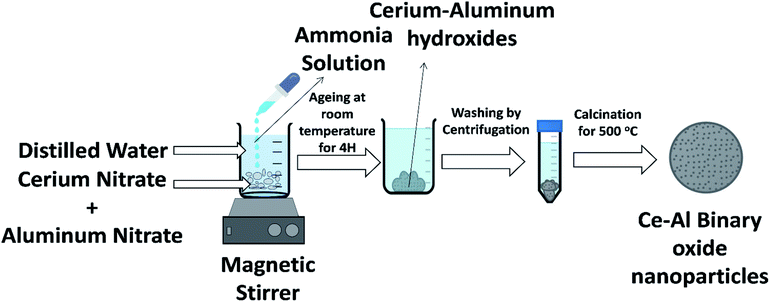 |
| | Fig. 1 Illustration of the synthesis of Ce–Al binary oxide nanoparticles. | |
2.3 Characterization of the prepared nanomaterials
The structure of the as-synthesized samples was examined by powder X-ray diffraction (XRD) using a Rigaku-Miniflex X-ray diffractometer with Cu-Kα radiation (λ = 0.15406 nm) in the 2θ range from 20° to 100°. Fourier transform infrared (FTIR) spectroscopy helped to analyze the material's microscopic details that induce the various vibration modes using a Perkin Elmer Spectrum 100 FTIR spectrophotometer at a wavelength ranging from 400 to 4000 cm−1 with KBr pellets as a reference point. To understand the thermal stability of the prepared nanoparticles by thermogravimetric analysis (TGA) and differential thermal analysis (DTA) study, a Perkin-Elmer TGA 4000 at a heating rate of 10 °C min−1 in the air atmosphere in a temperature range of 25–900 °C was used.
The synthesized nanomaterial's surface topography and chemical composition were analyzed using a scanning electron microscope equipped with an energy-dispersive X-ray microanalyser. The pH at the point of zero charge (pHpzc) of the material was calculated by a pH drift method. A solution containing 0.01 M of NaCl was prepared, and the pH was adjusted in the range from 2 to 10. Then, 0.15 g of the nanomaterial was added into 50 mL of solution, and the mixtures were stirred for 24 hours to reach adsorption equilibrium. The final pH of the solution was then calculated, and a graph was drawn between initial pHi and final pH − initial pH (ΔpH) to obtain pHpzc at which the charge on the surface of the nano adsorbent is zero. The specific surface area, pore-volume, and pore diameter were acquired by Brunauer–Emmett–Teller (BET) with nitrogen adsorption–desorption isotherm at 77 K using a Nova Station A, Quantachrome Corporation, USA. A BET isotherm was obtained by plotting a graph between a monolayer of adsorbed gas and the relative pressure, and by multiplying the monolayer capacity with the cross-sectional area of the adsorbate, the total surface area of the material was obtained. The pore volume was obtained by the quantity of adsorbed nitrogen vapour at relative pressure almost equal to unity, and the pore diameter was calculated by the BJH (Barrett–Joyner–Halenda) desorption model.
2.4 Batch adsorption experiments
After the stipulated contact time, the samples were centrifuged for 10 min at 9000–10000 rpm to separate the adsorbent. The concentration of the remaining fluoride in the solution was measured by the SPADNS method using a DR 5000 spectrophotometer (HACH Company, USA). This analytical technique can accomplish the minimum detection threshold of 0.02 mg L−1. The solution pH was varied by adding hydrochloric acid (HCl) and sodium hydroxide (NaOH) to the solution. Equilibrium adsorption capacity (qe in mg g−1), as well as percentage removal efficiency, was estimated by using the following eqn (1) and (2):| |
 | (1) |
| |
 | (2) |
where Ci is the initial fluoride concentration (mg L−1) at equilibrium, Ce is the concentration of fluoride remaining in the solution, V is the volume of fluoride solution (L), and m is the adsorbent mass (g).
2.5 Adsorption experiments
Batch adsorption studies were done to understand the adsorption isotherm, kinetics of the process, and the effect of dosage of nanoparticles, pH, and initial fluoride concentration. In the present method, 25 mL of fluoride-contaminated samples of different concentrations (for initial fluoride concentration experiments) was taken in 50 mL of the conical flask at a fixed pH of around 2.4. A desired amount of nanomaterials (for different dosage concentration experiments) was added and stirred at 180 rpm with varying intervals of time (for time-dependent experiments). Then, the nano adsorbent was separated by centrifugation technique, and the filtrate was tested for the remaining fluoride concentration (mg L−1). A separate adsorption experiment was studied at different initial pH values for 0.1 g L−1 of nano adsorbent dosage and initial fluoride concentration of 10 mg L−1 to determine a pH at which the highest adsorption capacity can be obtained. The pH of the solution was adjusted by the addition of 0.1 M HCl and 0.1 M NaOH solution in a drop-wise manner.
For the dosage experiment, 0.1–1.5 g L−1 of nano adsorbent was added to different initial fluoride concentrations of 10, 15, 25, and 35 mg L−1 at a pH of 2.4. For adsorption isotherm studies, 0.1–1 g L−1 of adsorbent was added to 25 mL solution of fluoride with an initial concentration range of 10–35 mg L−1 at an optimized pH of 2.4 and shaken for 4 hours in a mechanical shaker at a speed of 180 rpm to obtain the equilibrium value of the residual fluoride concentration. For kinetic studies, 10–35 mg L−1 of the initial fluoride concentration was taken, to which 0.1–1 g L−1 dosage of nano adsorbent was added. The solution was stirred on a shaker for pre-decided time intervals. After which, the nanoadsorbent was obtained from the filtrate by centrifugation and analyzed for residual fluoride concentrations. It is essential to mention that all the experiments were implemented out in triplicate, and the final data are presented as the mean value with a relative error of 5%.
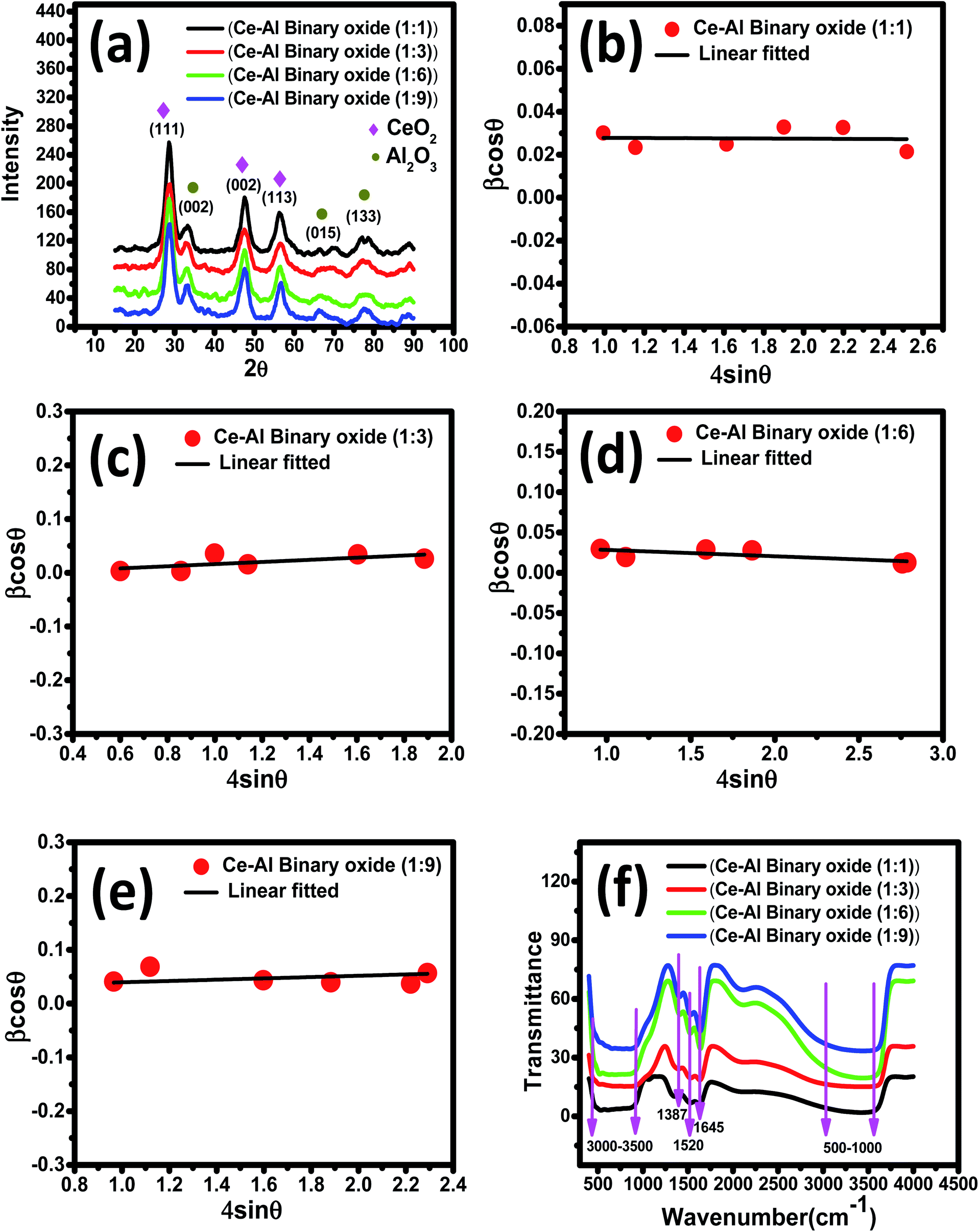
Table 1 Crystallite size and microstrain of Ce:Al binary oxides in molar concentrations of 1:1, 1:3, 1:6 and 1:9
| Molar concentration of Ce–Al |
Crystallite size (nm) |
| Debye–Scherrer method |
William–Hall method |
Microstrain, (ε) × 10−3 |
| 1:1 |
4.5 |
4.90 |
9.09 |
| 1:3 |
3.8 |
4.31 |
19.93 |
| 1:6 |
4.7 |
5.05 |
12.07 |
| 1:9 |
5.0 |
5.14 |
12.16 |
3 Results and discussion
3.1 Characterization of nanoadsorbents
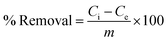
3.1.1 X-ray diffraction studies. XRD spectra of the series of prepared cerium-aluminum binary oxide nanomaterials calcined at 500 °C for 3 hours are depicted in Fig. 2(a). The graph shows the peaks of both cerium oxide and aluminium oxide in the resulting composite. All the peaks obtained were sharp and intensive, indicating the crystallinity of the nanomaterial.45–47 The diffraction peaks at 2θ = 28.78°, 47.56°, and 56.74° were indexed to the cubic structure of CeO2 as confirmed by JCPDS 01-081-0792 and the 2θ peaks at 33.59°, 66.67°, and 78.03° were indexed to the orthorhombic structure of Al2O3 as confirmed by JCPDS 96-100-0443. The XRD pattern showed no other additional peaks, indicating the purity of the prepared composite. Therefore, the resulting pattern supports the formation of Ce–Al binary oxides. A typical broadening in peak is observed, which may be due to quantum confinement.48–50 The average crystallite size was obtained from the Debye–Scherrer equation (eqn (3)) using the full-width at half-maximum (FWHM) of the most intense peak (111) of the cerium-aluminum binary oxide nanoparticle.| |
 | (3) |
where k = 0.94, D is the crystallite size (Å), λ (Å) is the X-ray wavelength of Cu Kα radiation (1.54178 Å), β is the FWHM (full width at half maximum), and θ is the angle of diffraction.51 The Williamson–Hall method is also used to estimate the microstrain and average crystallite size in materials using the following equations:52,53| |
 | (4) |
where λ is the X-ray wavelength, 0.9 is shape constant, and ε is the induced strain in the crystal, and β is the FWHM in radians. As illustrated in Fig. 2(b)–(e), the graphs between βcosθ on the y-axis and 4sinθ on the x-axis are shown and linearly fitted for all data. The intercept and slope of the line are used to compute the average crystallite size and microstrain. Table 1 summarizes these results. The discrepancy between the Debye–Scherrer and Williamson–Hall methods for determining the average crystallite size is a direct result of the strain.54,55
 |
| | Fig. 2 (a) XRD pattern of Ce–Al binary oxide nanomaterials at different molar concentrations; (b–e) Williamson–Hall plots for Ce–Al binary oxide nanoparticles at molar concentrations of 1:1, 1:3, 1:6, 1:9 respectively; and (f) Fourier transform infrared spectra of Ce–Al binary metal oxide nanoparticles at different molar concentrations. | |
Table 2 Comparative assessment of fluoride ion adsorption capacity of Ce–Al (1:6) binary oxides with other reported materials
| Adsorbent |
Adsorption capacity (mg g−1) |
Studied pH range |
Time taken to reach equilibrium (hour) |
Ref. |
| Magnesium–aluminum ternary oxide microspheres |
84.24 |
7.0 |
24 |
4 |
| Ce with metal organic frameworks (MOFs) |
4.88 and 4.91 |
6–7 |
0.5 |
111 |
| Iron–aluminum oxide/graphene oxide nanoparticles as |
64.72 |
64.72 |
3 |
21 |
| Ce–Zr oxide nanospheres encapsulated calcium alginate beads |
137.6 |
7.0 |
10 |
22 |
| Iron aluminum nanocomposite |
42.95 |
6.9 |
1.33 |
23 |
| Al2O3 nanoparticles |
3.82 |
4.7 |
1.5 |
24 |
| Cerium(IV)- incorporated hydrous iron(III) oxide |
32.62 |
7.0 |
2 |
75 |
| MnO2–Al2O3 composite material |
18.6 |
7.0 |
1 |
112 |
| Ce–Al binary oxide nanoparticles |
384.6 |
2.4 |
4 |
This study |
3.1.2 Fourier transform infrared spectra. The FTIR spectrum of a series of Ce–Al binary oxides at different molar concentrations is shown in Fig. 2(f), which further confirms the successful synthesis of the material. The broad band was obtained between 3000 and 3500 cm−1 in the spectrum presumptively assigned to the stretching modes of vibration of water adsorbed. The peak at 1520 and 1645 cm−1 is attributed to the bending vibration mode of the OH group present on metal oxides.56,57 The vibration at around 1387 cm−1 is assigned to the nitrate group due to some residues left from cerium nitrate and aluminum nitrate used during the synthesis process.58 As reported in the literature, the FTIR spectrum of cerium oxides shows bands below 700 cm−1, which can be ascribed to the stretching vibration of the Ce–O bond.59–62 The stretching vibration modes of aluminium oxide bonds are obtained in the range of 580–636 cm−1.63,64 Thus, the broad band seen in the range of 500–1000 cm−1 could be attributed to bending and stretching modes of vibration of the M–O bond, confirming the formation of Ce–O–Al bonds in the material.65
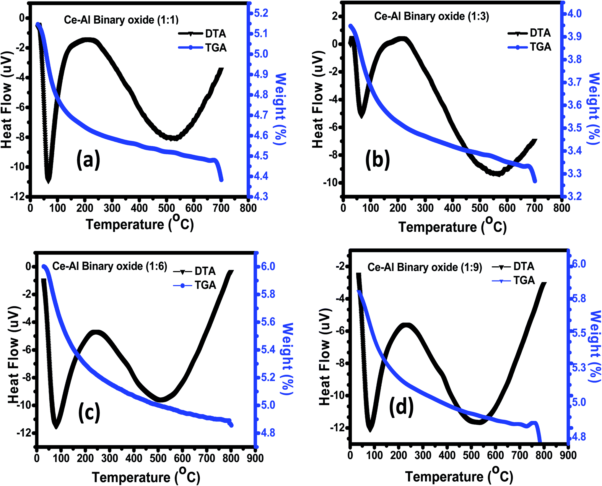
3.1.3 Thermogravimetric analysis (TGA)/differential thermal analysis (DTA). The thermal decomposition and stability of the prepared binary oxide nanomaterial at different molar concentrations were studied using TGA/DTA, as shown in Fig. 3(a)–(d). The spectrum of all molar concentrations of Ce–Al binary oxides shows continuous loss of weight from 30 °C to 800 °C. The sample (a–d) shows a weight loss of 9.8%, 12.8%, 13.5%, and 10.5% respectively, below 250 °C along with an endothermic peak at roughly 100 °C. This can be accredited to the removal of the water molecules present in the precursor material. Between the temperature range of 300 °C to 750 °C, all the material shows a slight weight loss of approximately 3–5%. The DTA graph shows an endothermic peak at around 500 °C due to thermal degradation.
 |
| | Fig. 3 (a–d) TGA/DTA curve of Ce–Al binary oxides in different molar concentrations. | |
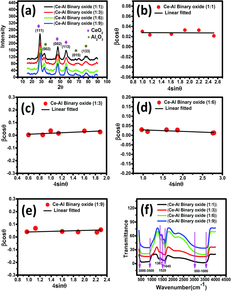
3.1.4 Scanning electron microscopy with energy-dispersive spectroscopy. The surface morphology and elemental constituents of the prepared nanomaterial were analyzed by SEM-EDAX (Fig. 4). The SEM micrograph showed that nanoparticles are agglomerated and of varying sizes (approx. from 4 to 5 nm) and shapes.
 |
| | Fig. 4 SEM micrographs and EDS pattern for Ce–Al binary oxide nanoparticle with atomic percentage of the elements. | |
The SEM-EDX spectrum signifies the presence of cerium and aluminum with no other impurities. This agrees with our desire to synthesize the pure material. From the analytical data, the empirical formula of the binary oxide was obtained as Ce–Al3.3–O9.62.
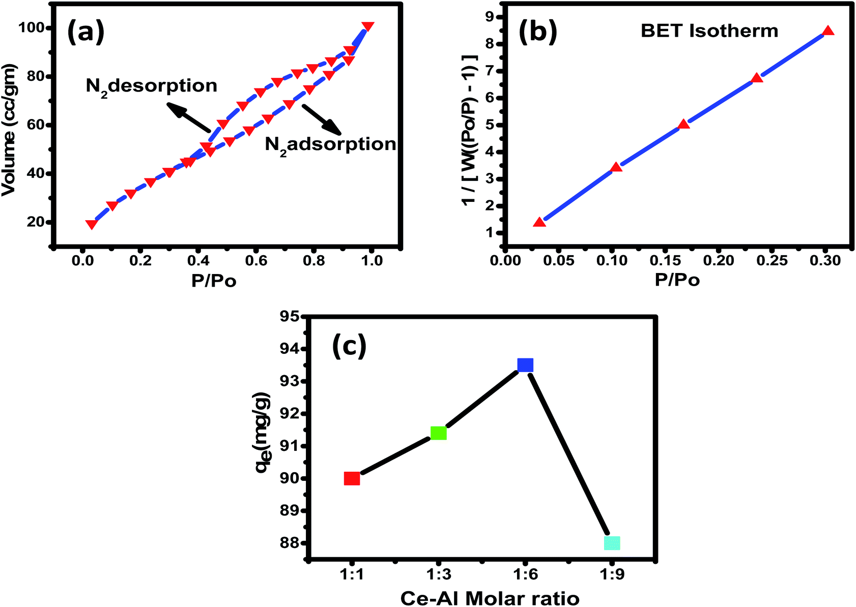
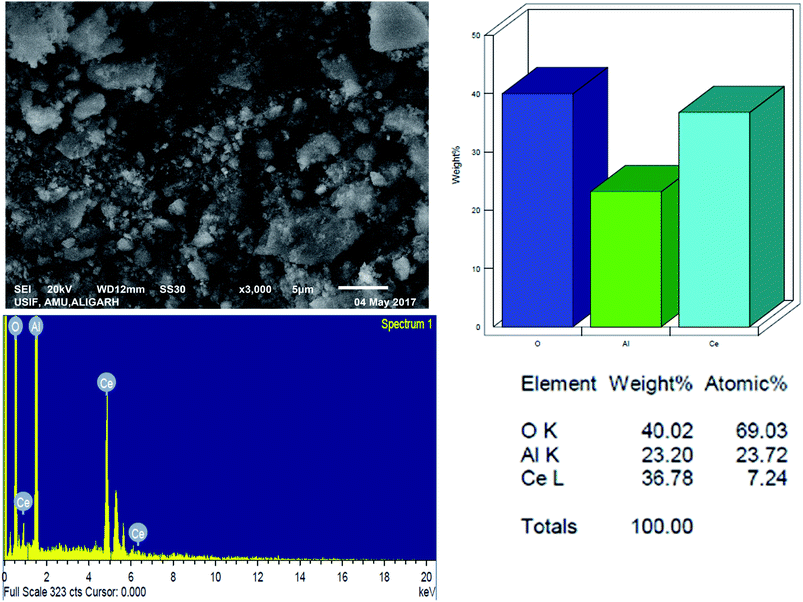
3.1.5 Specific surface area and pore size distribution analyses. Brunauer–Emmett–Teller's (BET) study was analyzed to calculate the surface area of Ce–Al binary oxide nanoparticles. The surface area and porosity of the material play a significant role in establishing its adsorbent capacity. As estimated by the nitrogen adsorption isotherm, the surface area was found to be 130.7 m2 g−1. Fig. 5(a) and (b) show the nitrogen adsorption–desorption isotherm of the synthesized nanomaterial and pore size distribution curve, respectively. The isotherm shows type IV with hysteresis loops of type H2 classified by BDDT (Brunauer–Deming–Deming–Teller) in 1940 and IUPAC recommendations in 1985.66,67 The pore volume and average pore diameter were determined to be 0.141 cc per g and 3.673 nm, respectively, indicating the surface to be mesoporous. The pore diameter of an adsorbent as observed is greater than the average pore diameter of fluoride ions68,69 (0.133 nm), suggesting F− to readily enter the adsorbent's pores. A graph is plotted between P/P0 and 1/[W(P0/P) − 1], which shows linear variation, suggesting that the adsorbent is highly porous.
 |
| | Fig. 5 (a) Plots of N2 (vapour) adsorption (black)–desorption (red), with a pore volume of 0.141 cc per g; (b) pore size distribution of Ce–Al binary oxide with surface area = 130.7 m2 g; (c) adsorption of fluoride on the hybrid adsorbents prepared at different Ce:Al molar ratios (adsorption conditions: 0.1 g L−1 adsorbent in 25 mL of 15 mg L−1 of fluoride solution at pH 6 and 30 °C for 4 hours). | |
3.2 Optimising Ce–Al molar concentration in the binary oxide adsorbent
3.2.1 Synergistic reactions. Fluoride removal capacity for the prepared Ce–Al binary oxide nanoparticles was studied with four different molar concentrations of aluminum, keeping cerium content constant, as shown in Fig. 6. The fluoride adsorption capacity can be observed to increase first and then decrease with the increase in aluminum content ratio from 1:6 to 1:9, and the maximum fluoride adsorption capacity was observed for the 1:6 molar concentration of Ce–Al binary oxide nanoparticles. The Ce–Al binary oxide nanomaterial prepared at Ce–Al molar ratios of 1:1, 1:3, 1:6, and 1:9 have the crystallite size calculated to be 4.5 nm, 3.8 nm, 4.7 nm, and 5 nm, respectively, and adsorption capacities of 90 mg g−1, 91.4 mg g−1, 93.5 mg g−1 and 88 mg g−1 respectively. The data show that the crystallite size, generally related to the surface area is not the primary factor affecting the adsorption capacity. Even though the Ce–Al binary oxide in the molar ratio of 1:3 has the smallest crystallite size, it does not guarantee a high adsorption capacity. This behavior could be attributed to the synergistic relationship between cerium and aluminum oxides to form the specific structure of the adsorbent, which is favorable for fluoride adsorption.70–72 Such a trend has also been shown by other researchers.73–77 Thus, Ce–Al (1:6) was selected for further experiments as it showed maximum adsorption capacity for fluoride.
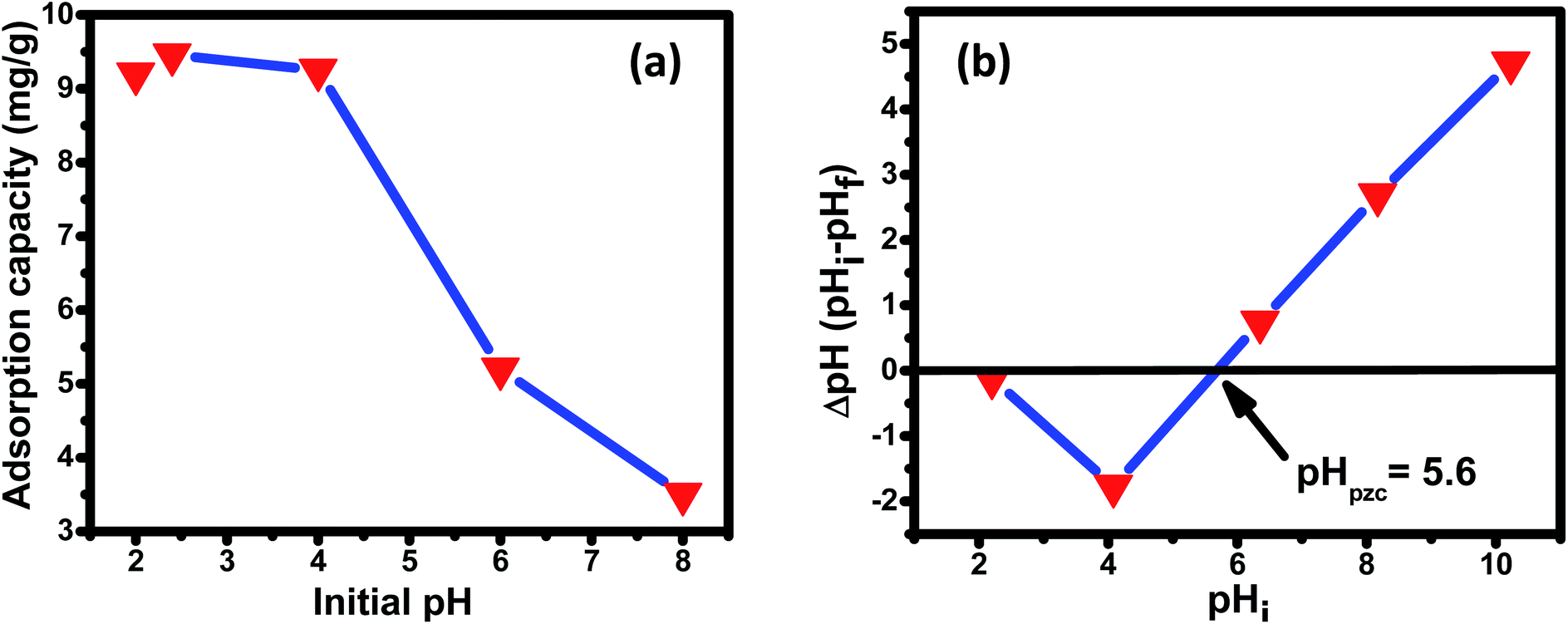
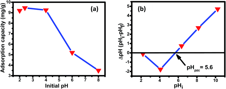 |
| | Fig. 6 (a) Effect of the initial solution pH on the adsorption of fluoride over the Ce–Al binary oxide nanomaterial at an initial fluoride concentration of 10 mg L−1 with 1 g L−1 dosage of adsorbent. (b) Plot of ΔpH versus pHi for the estimation of pHZPC of Ce–Al binary oxide. | |
3.3 Adsorption performance
3.3.1 Effect of pH, point of zero charge (pHzpc), and mechanism of adsorption. The initial pH of the solution (pHi) and point of zero charge (pHzpc) profoundly affect the adsorption capacity of the adsorbate on the adsorbent surface. The effect of initial pH on the adsorption capacity is shown in Fig. 6(a). The graph depicts the highest adsorption capacity of 9.46 mg g−1 at lower pH (2.4), i.e., under acidic conditions, and a noteworthy reduction in adsorption capacity under basic conditions. This result agrees with other research works published signifying a high adoption capacity of fluoride at low pH.78,79 Predominantly, the adsorption mechanism follows anion exchange with hydroxyl ions or electrostatic attractions. The point of zero charge (pHzpc) is when the surface charge of the adsorbent is zero.80,81 The pHzpc value for the prepared nanomaterial is 5.6, indicating that below this pH, the surface charge is positive and above this pH, negative. It can also be observed [Fig. 6(a)] that the adsorbent capacity decreased significantly above pHzpc, signifying that at pH > 5.6, there is strong electrostatic repulsion between fluoride ions and the negatively charged surface of the nano adsorbent. Fluoride adsorption between the pH range of 2–8 can be understood by the following mechanisms. At pH below pHzpc (pH < pHzpc), the adsorption mechanism essentially follows either electrostatic/coulombic attraction or anion exchange reaction. As observed in the figure, the adsorption capacity is highest at pH 2.4, which is sufficiently less than the pHzpc value, suggesting the mechanism to be electrostatic/coulombic attraction between the positively charged adsorbent surface and the negatively charged fluoride ion (R1). The adsorption capacity decreases in the pH range of 3.5–5 (below pHzpc value) because of the changes in the availability of positive charge surface, indicating that the adsorption mechanism now follows the ion-exchange process between (R2). At higher pH, i.e., pH ≫ pHzpc, adsorption capacity is found to decrease drastically. This is because, at pH above pHzpc, the surface of the adsorbent is essentially negatively charged, leading to repulsion between the negatively charged binary oxide nano adsorbent surface and negatively charged fluoride anion (R3). There is increased opposition between abundantly present OH− and F− for active adsorption sites at higher pH, resulting in decreased adsorption capacity.
| (CeO2–Al2O3)–OH ≡ (M–OH)s + H+aqs → (M–OH2)+ |
| | |
(M–OH2)s+ + Faq− → (M–OH2)+–F− + H2O
| (R1) |
| | |
(M–OH)s + F− → M–F + OH−
| (R2) |
| | |
(M–OH)s + F− + OH−aq → M–O− + H2O + F−
| (R3) |
It is also worth noting that above pHpzc, the adsorption capacity drastically decreased, indicating that electrostatic attraction could be the primary mechanism for fluoride adsorption on the surface of Ce–Al binary oxide nanomaterials. This is also found in accordance with several past research works.21,23,54,61,82
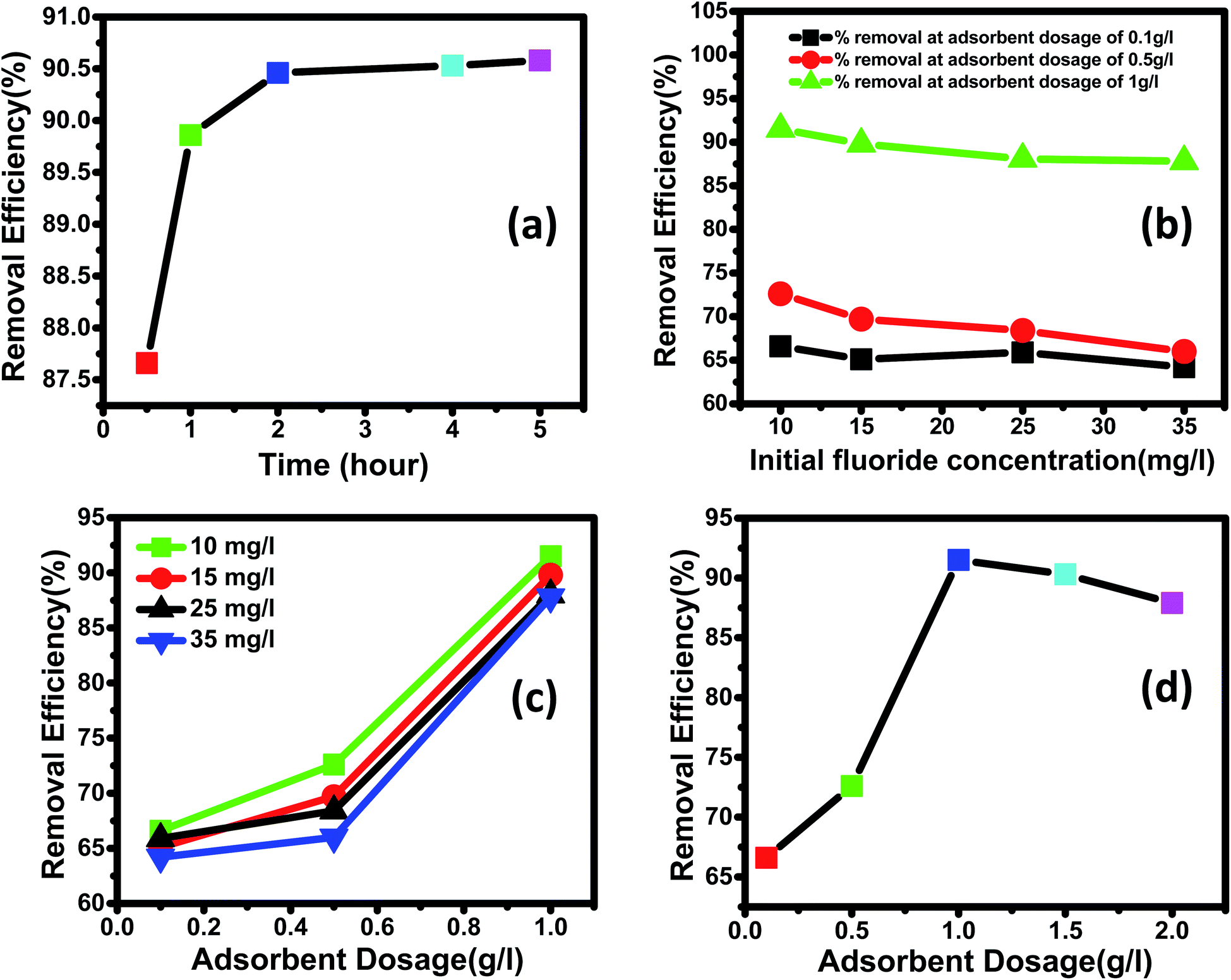
3.3.2 Effect of the initial fluoride concentration. The adsorption rate is a function of the adsorbate's initial concentration, making it a critical parameter for efficient adsorption. The influence of initial concentration on the adsorption of fluoride ions by Ce–Al binary oxide nanoadsorbents was examined using three different adsorbent doses and varied solution concentrations of 10, 15, 25, and 35 mg L−1, as shown in the figure. It can be inferred from Fig. 7(b) that the removal efficiency of the adsorbent material declines with an increase in the initial concentration of fluoride ions in the solution. The behavior mentioned above is the direct result of filling up all active sites present on the surface of nanoadsorbents with an increase in fluoride concentration.83
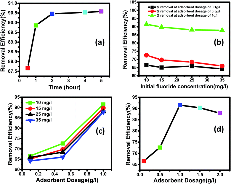 |
| | Fig. 7 (a) Effect of contact time on the fluoride removal (%) with time (adsorbent dose: 1 g L−1; initial fluoride concentration of 15 mg L; adsorption duration: 0.5–4 hours; temperature: 30 °C; pH: 2.4). (b) Effect of initial concentration on the fluoride removal efficiency (%) (adsorbent dose: 0.1 g L−1, 0.5 g L−1 and 1 g L−1; initial fluoride concentration: 10–35 mg L−1; adsorption duration: 4 hours; temperature: 30 °C; pH: 2.4). (c) Effect of the adsorbent dose on fluoride removal efficiency (%) (initial fluoride concentration: 10, 15, 25 and 35 mg L−1; adsorbent dose: 0.1–1 g L−1; adsorption duration: 4 hours; temperature: 30 °C; pH: 2.4). (d) Decrease in removal efficiency (%) with the increase in adsorbent dosage beyond an optimum dose (initial fluoride concentration: 10 mg L−1; adsorbent dose: 0.1–2 g L−1; adsorption duration: 4 hours; temperature: 30 °C; pH: 2.4). | |
Similar adsorption patterns are reported by various researchers.84,85
3.3.3 Effect of contact time. In this work, the influence of contact time as a primary requirement to determine the equilibrium time for maximum removal efficiency and establish the process kinetics was studied at temperatures of 30 °C, pH 2.4, initial Fl-concentration of 15 mg L−1, and adsorbent dosage of 1 g L−1 for 0.5, 1, 2, 4, and 5 hours. As clear from Fig. 7(a), the fluoride was adsorbed rapidly within the first hour of the adsorption process, then subsequently at a relatively slower rate. More significant amounts of fluoride were adsorbed during the first hour because fluoride ions instantly bind to the readily available active sites on the adsorbent's outer surface. The progressive diffusion of fluoride ions into the interior surface of the porous Ce–Al binary oxide adsorbent causes the slower uptake of fluoride after 1 hour. Due to the fast initial stage adsorption, which was followed by a second stage with a relatively slow adsorption process until equilibrium was established, the adsorption process for fluoride ion was detected even in a short period of time. According to numerous published studies by different researchers, equilibrium is reached when the percentage of fluoride removal does not improve significantly despite the prolonged contact duration.86–88 The reaction time for the supporting tests was fixed at 4 hours because no significant change in adsorption was seen after 4 hours in this investigation.
3.3.4 Effect of adsorbent dosage on fluoride removal. Dosage of adsorbent has a profound effect on the removal efficiency of fluoride, as shown in Fig. 7(c) and (d). The adsorbent dosage varied between 0.1 g L−1 and 1.5 g L−1 at different concentrations of fluoride ranging from 10 to 35 mg L−1. All the experiments were studied at a fixed pH of 2.4 and a contact time of 4 hours. As shown in Fig. 7(c) for all fluoride concentrations, the removal efficiency increased with an increase in the dosage of the nanomaterial. This is because increasing the dosage increases the number of active adsorption sites, leading to increased removal efficiency, as illustrated in previous works by different researchers.89,90 Fig. 7(d) shows that maximum removal of 91.5% observed for 1 g L−1 dosage of adsorbent at 10 mg L−1 of initial fluoride concentration.Further increasing the dose of adsorbent did not improve the removal efficiency. This is because of the non-availability of active sites on the adsorbent and the establishment of equilibrium between the fluoride ions on the adsorbent and in the solution. Such behavior has also been reported by other researchers.4,91,92
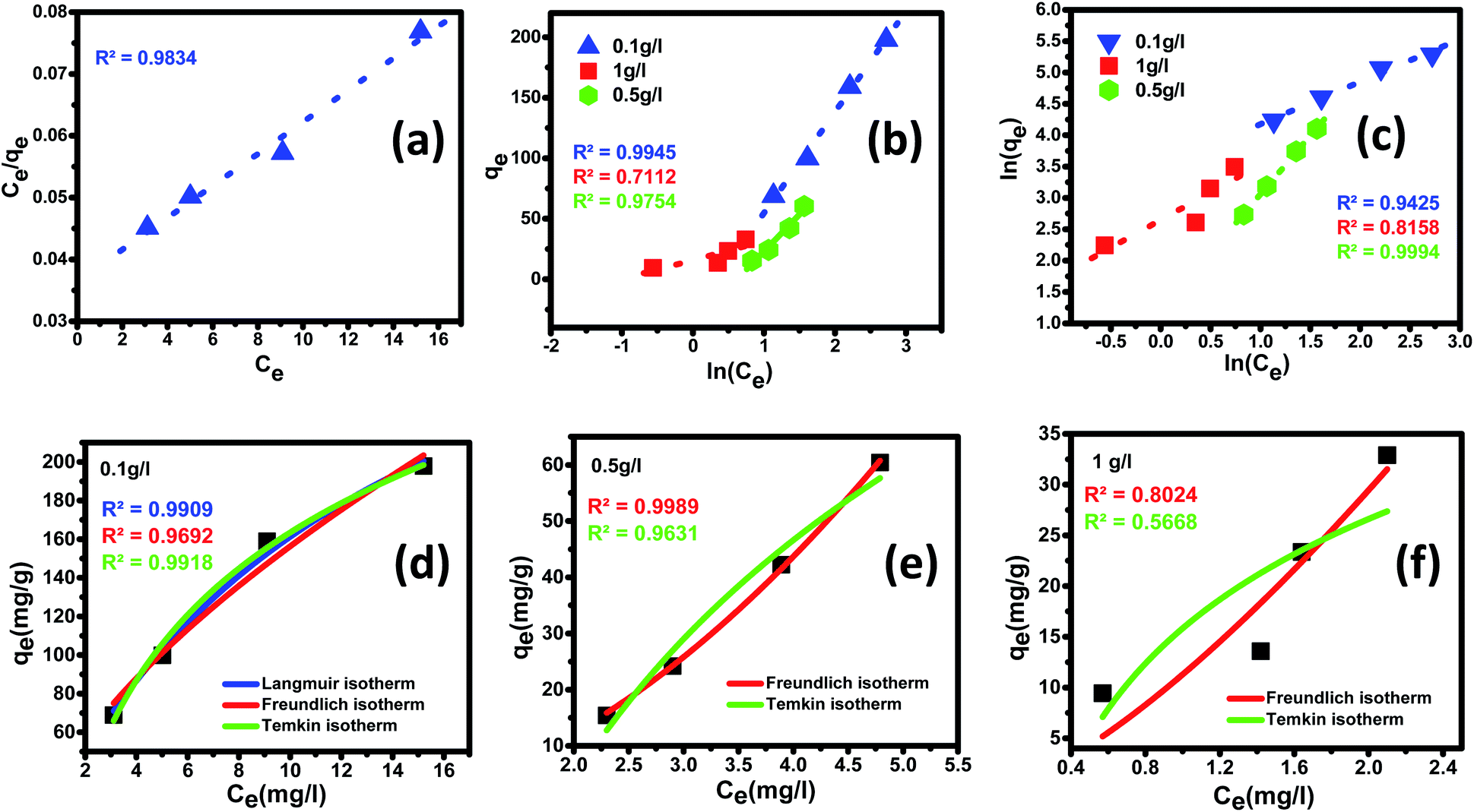
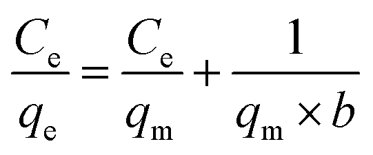
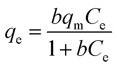
3.3.5 Adsorption isotherm. The adsorption process establishes a dynamic equilibrium between the distribution of the adsorbate on the surface of the adsorbent. To understand the process of adsorption and demonstrate the efficiency of the nanomaterial, adsorption isotherm holds a crucial place. Langmuir and Freundlich isotherms are the most common types of adsorption models employed to study the mechanism of the adsorption process and surface properties of the adsorbent material. The acquired equilibrium data were analyzed by fitting linear equations of the most widely accepted isotherms such as Langmuir, Freundlich, and Temkin isotherms at 25 ± 5 °C. The difference between these three models is that in the Langmuir model, it assumes that heat of adsorption has no change throughout the adsorption process, whereas, in Freundlich, isotherm presumes heat of adsorption to logarithmically decrease, while in the Temkin isotherm, the heat of adsorption decreases linearly with surface coverage.93,94 These isotherms provide insight into the adsorbent's affinity to the adsorbate, thereby giving direction to optimizing the prepared nanomaterial as an adsorbent material. Adsorption isotherms corresponding to the most suitable fit for experimental data obtained for fluoride adsorption at an optimum pH of 2.4 are for linear fitting are demonstrated in Fig. 8(a)–(c) as well as non-linear fitting are shown in Fig. 8 (d)–(f) along with the fitting parameters calculated are outlined in Tables 3 and 4.
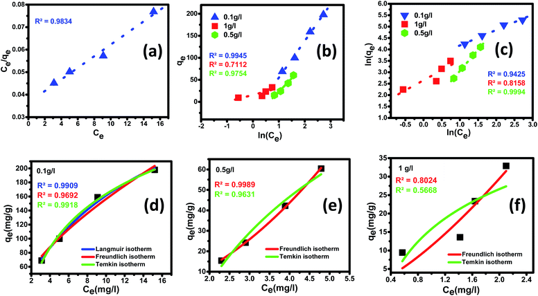 |
| | Fig. 8 Adsorption equilibrium isotherms for fluoride ion removal by Ce–Al (1:6) binary oxide nanoadsorbent and the data fitting to linear (a) Langmuir, (b) Freundlich and (c) Temkin isotherm models along with nonlinear fitting of (d–f) Langmuir, Freundlich and Temkin isotherm models for different adsorbent doses. | |
Table 3 Langmuir isotherms (linear and non-linear fitting) parameters for the adsorption of fluoride ions onto Ce–Al (1:3) binary oxide nanoparticles
| Linear fitting |
| Langmuir isotherm parameters |
RL value for different initial concentrations |
| qmax (mg g−1) |
b (L mg−1) |
R2 |
10 mg L−1 |
15 mg L−1 |
25 mg L−1 |
35 mg L−1 |
| 384.6 |
0.07143 |
0.9834 |
0.583333 |
0.482759 |
0.358974 |
0.285714 |
| Non-linear model |
| Best-fit values |
| qmax (mg g−1) |
377.9 |
| b |
0.07443 |
|
| Std. error |
| qmax (mg g−1) |
3.974 |
| b |
0.01306 |
|
| 95%Confidence intervals |
| qmax (mg g−1) |
214.46 to 541.24 |
| b |
0.01823 to 0.13063 |
|
| Goodness of fit |
| Degrees of freedom |
2 |
| R2 |
0.99098 |
| Residual sum of squares |
60.62893 |
| Sy.x |
5.50586 |
| Number of points analyzed |
4 |
Table 4 Freundlich and Temkin isotherms (linear and non-linear fitting) parameters for the adsorption of fluoride ions onto Ce–Al (1:3) binary oxide nanoadsorbents
| Freundlich isotherm |
| Isotherm models |
Dosage of Ce–Al binary oxides nanoparticles |
| 0.1 g L−1 |
0.5 g L−1 |
1 g L−1 |
| Linear fitting |
| Kf (mg g−1) |
29.36 |
3.281 |
14.12 |
| n |
0.49 |
0.535 |
0.132 |
| R2 |
0.9425 |
0.9994 |
0.8158 |
|
| Non-linear model |
| Best-fit values |
| Kf (mg g−1) |
36.79 |
3.455 |
11.280 |
| n |
1.591 |
0.546 |
0.722 |
| Std. error |
| Kf (mg g−1) |
6.2989 |
0.2069 |
3.610 |
| n |
0.1841 |
0.0125 |
0.269 |
| 95%Confidence intervals |
| Kf (mg g−1) |
9.68526 to 63.88918 |
2.565 to 4.34597 |
4.25203 to 26.8132 |
| n |
0.79956 to 2.38373 |
0.49258 to 0.60024 |
0.43964 to 1.8835 |
| Goodness of fit |
| Degrees of freedom |
2 |
2 |
2 |
| R2 |
0.96926 |
0.99895 |
0.80244 |
| Residual sum of squares |
206.6068 |
0.83523 |
43.5297 |
| Sy.x |
10.16383 |
0.64623 |
4.66528 |
| Number of points analyzed |
4 |
4 |
4 |
| Temkin isotherm |
| Isotherm models |
Dosage of Ce–Al binary oxides nanoparticles |
| 0.1 g L−1 |
0.5 g L−1 |
1 g L−1 |
| Linear fitting |
| AT (L g−1) |
0.715 |
0.4018 |
1.1001 |
| b |
29.81 |
41.869 |
164.612 |
| R2 |
0.9945 |
0.9754 |
0.7112 |
|
| Non-linear model |
| Best-fit values |
| AT (L g−1) |
0.7081 |
0.5357 |
2.7668 |
| b |
30.668 |
41.869 |
164.616 |
| Std. error |
| AT (L g−1) |
0.06262 |
0.03888 |
1.70719 |
| n |
1.614 |
4.72256 |
4.54623 |
| 95%Confidence intervals |
| AT (L g−1) |
0.43874 to 0.97758 |
0.36839 to 0.70297 |
4.57868 to 10.1122 |
| b |
23.72331 to 37.61226 |
21.54985 to 62.18889 |
156.13096 to 485.36215 |
| Goodness of fit |
| Degrees of freedom |
2 |
2 |
2 |
| R2 |
0.99182 |
0.96314 |
0.5668 |
| Residual sum of squares |
54.99617 |
29.43451 |
95.45091 |
| Sy.x |
5.24386 |
3.83631 |
6.90836 |
| Number of points analyzed |
4 |
4 |
4 |
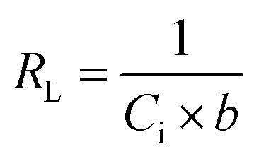
Langmuir adsorption isotherm gives information that the process of adsorption occurs on a homogenous surface with monolayer adsorption occurring as all the adsorption sites are the same and equivalent in energy. The isotherm assumes there is no interaction between the adsorbent and the adsorbate.95–97 The mathematical representations of linear and non-linear forms of Langmuir equations are represented using eqn (5) and (6), respectively.61,98
| |
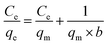 | (5) |
| |
 | (6) |
where
Ce (mg L
−1) is the concentration of the adsorbate at equilibrium,
qe (mg g
−1) is the equilibrium adsorption capacity,
qm (mg g
−1) is the maximum adsorption capacity, and
b (L mg
−1) is the Langmuir constant associated with the free energy of adsorption.
99
A linear graph was plotted between Ce/qe and Ce, and from the straight-line values of Langmuir parameters, qm and b were obtained, and a non-linear plot between Ce vs. qe is also shown in Fig. 8(d).
Langmuir equation has been successfully employed to calculate the maximum adsorption capacity for various nanoadsorbents.100,101 To establish the Langmuir adsorption model's favorability, a dimensionless separating factor RL is represented using eqn (5).102 The calculated isotherm parameters, including qm and b for linear and non-linear Langmuir fit, are summarized in Table 3.
| |
 | (7) |
where
Ci (mg L
−1) is the initial adsorbate concentration and
b (L mg
−1) is the Langmuir constant. The process of adsorption is considered favorable when RL's value lies between 0 and 1. When the value of
RL is more than 1, then adsorption is considered to be unfavorable; when the value of
RL is equal to 1, then the process of adsorption is linear; when the value of
RL is 0, the adsorption process is irreversible and, when the value of
RL lies in the range of 0–1, then it can be concluded that the adsorption process is favorable.
In the present study, maximum adsorption capacity (qm) as calculated by fitting experimental data to linear and non-linear Langmuir equations was observed to be 384.6 mg g−1, 377.8 mg g−1, respectively and the value of correlation coefficient R2 was obtained to be 0.9834 and 0.9909 respectively. The value of RL in this study lies in the range of 0.2 and 0.7, suggesting fluoride adsorption on Ce–Al nanoparticles to be favorable in nature.103
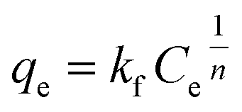
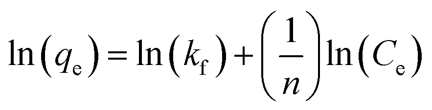
Freundlich isotherm model assumes that the adsorption process occurring is the multilayer on the heterogeneous adsorbent. The model assumes that all adsorption sites have unequal energy, which varies exponentially, leading to many adsorbate layers being formed on the surface of the adsorbent. Mathematically, non-linear and linear equations of Freundlich isotherm can be represented by eqn (8) and (9).104
| |
 | (8) |
Eqn (8) can be linearized and written as follows:105
| |
 | (9) |
where
Kf (mg g
−1) is the adsorption capacity,
qe is the adsorption capacity at equilibrium, and
n (L mg
−1) is the Freundlich constant related to the intensity of adsorption.
87 If the value of 1/
n < 1, then chemical adsorption occurs, whereas when 1 <
n < 10, then physical adsorption is favored.
106 A graph is plotted between ln
qe versus ln
Ce; Freundlich parameters such as
Kf and
n as calculated from the intercept and slope of linear plot and non-linear fittings are summarized in
Table 4.
In the present study, the fitting of experimental data with the isotherm model yielded a value of regression coefficient R2 to be 0.999, as shown in Fig. 8(b). The Freundlich isotherm model was found to be a better fit than the Langmuir model from the regression coefficient value. As given in Table 4, the heterogeneity factor (n) is less than one, suggesting that adsorption processes are reasonably heterogeneous in nature.107
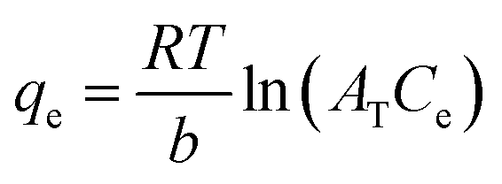
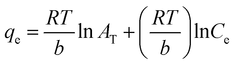
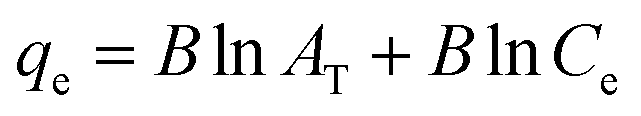
The Temkin adsorption model surmises that the heat of adsorption declines linearly with a further increase in the surface coverage due to adsorbate–adsorbent interaction.93 Temkin adsorption isotherm is valid only when ion concentrations are neither too high nor too low.108 The model elucidates the process of interaction between adsorbate and adsorbent to be chemisorption in nature.4 The following equation can express the adsorption model in a non-linear form:109
| |
 | (10) |
The above equation can be linearized and written as follows:
| |
 | (11) |
| |
 | (12) |
| |
 | (13) |
where
AT (L g
−1) is the equilibrium binding constant of Temkin isotherm,
b (J mol
−1) is the Temkin isotherm constant,
R is the universal gas constant having a value of 8.314 J mol
−1 K
−1,
T is the temperature at 298 K, and
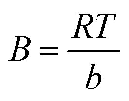
B is the constant related to the heat of adsorption expressed by
B =
RT/
b. A linear graph obtained by plotting adsorption capacity at equilibrium (
qe)
versus ln
Ce, and the Temkin parameters are obtained from the slope (b) and intercept (
AT).
108,110
In this study, the Temkin isotherm can explain the fluoride adsorption on the surface of an adsorbent. The value of R2 obtained from both linear and non-linear fit varies from 0.711 to 0.99 (Fig. 8(d)–(f) and Table 4), which is relatively closer to the Freundlich isotherm.
The order of isotherm adsorption models that fit best (for both linear and non-linear fitting) to the experimental data was determined to be Freundlich > Temkin > Langmuir based on the value of the regression coefficient (R2).
From the above-mentioned results obtained, it can be deduced that the mechanism of adsorption is a composite process, which includes electrostatic interaction with chemisorption having multilayer convergence on the heterogeneous Ce–Al binary oxide surface.
For comparison, the maximum adsorption capacity (qmax) values of fluoride ions on other materials are listed in Table 2. Clearly, the nanostructured Ce–Al binary oxide as a nanoadsorbent shows an excellent adsorption capacity of 384.6 mg g−1 compared to those of other adsorbents. As a result, this adsorbent has good prospect for fluoride ion removal from contaminated water.
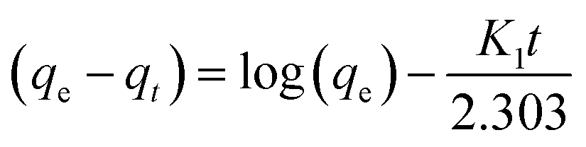
3.3.6 Kinetics analysis. To determine the adsorption mechanism, time-dependent studies were carried out to determine the rate-controlling step. For this experiment, four different initial concentrations (10 ppm, 15 ppm, 25 ppm, and 35 ppm) of fluoride with three different nanoparticles' dosages (0.1 g L−1, 0.5 g L−1, and 1 g L−1) were taken at an optimum pH of 2.4.To establish the reaction mechanism for fluoride adsorption on the Ce–Al binary oxide nanoadsorbent, pseudo-first-order, pseudo-second-order, and intraparticle diffusion rate equations were applied to study the kinetics of the process, as shown in Fig. 9.
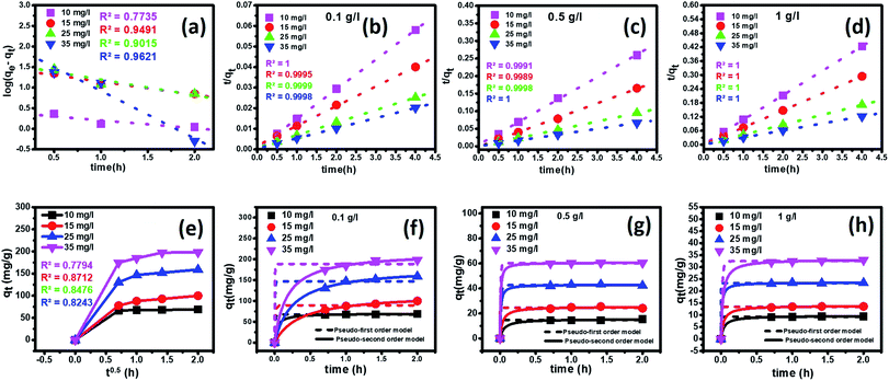 |
| | Fig. 9 Effect of contact time on the adsorption of fluoride ions by the Ce–Al (1:6) binary oxide nanoadsorbent at 25 ± 1 °C at an optimum pH 2.6 with linear kinetic models of (a) pseudo-first-order, (b–d) pseudo-second-order (e) intraparticle diffusion kinetic plot and (f–h) pseudo-first-order and pseudo-second-order nonlinear fitting for different adsorbent doses. | |
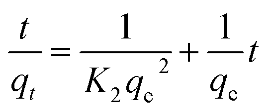
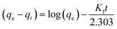
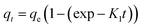
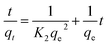
Linear and non-linear forms of pseudo-first-order and pseudo-second-order kinetic models were fitted to the experimental data for fluoride adsorption, which can be shown using eqn (14)–(17) respectively:81,113
| |
 | (14) |
| |
 | (15) |
where
qe (mg g
−1) and
qt (mg g
−1) are the equilibrium adsorption capacity, and at any time,
K1 (g mg
−1 h
−1) is the pseudo-first-order rate constant. A linear graph of pseudo-first-order kinetics [
Fig. 9(a)] is obtained between log(
qe −
qt) and time, from which
qe and
K1 can be obtained from the intercept and slope of the graph.
| |
 | (16) |
| |
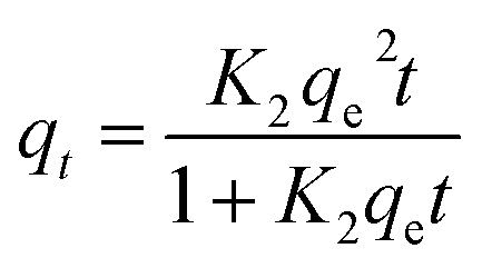
 | (17) |
A linear graph of pseudo-second-order kinetics [Fig. 9(b)–(d)] was plotted between t/qt and t, from which the value of constants k2 (g mg−1 h−1) and qe (mg g−1) can be determined.48 The pseudo-second-order kinetic equation is usually applied for chemisorption kinetics from liquid solutions.114 Fig. 9(f)–(h) show the non-linear fitting of pseudo-first-order and pseudo-second-order kinetic models. Adsorption kinetic parameters determined for these two kinetic models are presented in Tables S1 and S2.†
In the current study, it can be observed that for all three different dosages of nanoadsorbent, the R2 values obtained from the pseudo-second-order model (R2 linear = 0.9999–1.000 and R2 non-linear = 0.9995–1) are greater than those obtained from the pseudo-first-order model (R2 linear = 0.5714–0.9960 and R2 non-linear = 0.9478–0.9997). It is also worth noting that the experimental and calculated qe values from the pseudo-second-order model were closely correlated.
It can be observed that there is a decrease in the values of K2 with an increase in the initial concentrations of fluoride ions for all three adsorbent dosages. This occurs because of faster adsorption from dilute solutions, as fewer fluoride ions migrate to the adsorption sites in contrast to concentrated solutions.81,96,115
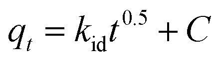
The intra-particle diffusion kinetic model was introduced by Weber–Morris, which explains the diffusion mechanism in which adsorbate molecules diffuse after adsorption on the surface, which diffuses into the pores of the adsorbent.116 According to the following equation, the experimental data obtained were fitted to the intraparticle diffusion plot to understand the diffusion mechanism.
| |
 | (18) |
where
qt (mg g
−1) is the quantity of fluoride adsorbed at a time,
kid (mg g
−1 hour
−0.5) is the intraparticle diffusion rate constant, and
C (mg g
−1) is a constant that represents the boundary layer thickness, which can be calculated by plotting
qt versus t0.5. The parameters of the kinetic model
eqn (18) as estimated from the plots are demonstrated in Table S3
†. According to this model, if a graph shows multi-linearity, then more adsorption processes are involved, and the intra-particle diffusion process is not the rate-limiting step. A multi-linear plot was obtained in the present study, indicating the diffusion process occurring in three steps [
Fig. 9(e)]. In the first step, we observe a sharp portion representing external mass transfer
via instantaneous adsorption. The next step shows a gradual adsorption process representing intra-particle or pore diffusion as a rate-controlling step. The last step shows a plateau, an equilibrium stage where diffusion is slow as the amount of adsorbate also decreases. It can be observed that for all three different dosages of nanoadsorbent, the
kid values increased with an increase in the initial fluoride concentrations from 10 mg L
−1 to 35 mg L
−1 (Table S3
†). However, the linear plots did not pass through the origin, denoting a complex situation in which both film diffusion and intra-particle diffusion contribute to the rate-limiting step.
102 The magnitude of
C increases with the increase in initial fluoride ion concentrations for all three different adsorbent doses.
81 This indicates an increase in boundary layer effects.
117 Similar multi-linear plots are found in the literature by various researchers.
118,119 Thus, the results indicated that intraparticle diffusion is not the only deciding factor and the adsorption mechanism followed pseudo-second-order kinetic model with a good correlation.
4 Conclusions
In the proposed study, we have successfully prepared cerium-aluminum binary metal oxide nanoparticles by a simple co-precipitation method. The average crystallite size of 4.70 nm was calculated from XRD, which demonstrated an excellent capacity for fluoride adsorption. The effect of molar concentrations of aluminum content in the binary oxides on the fluoride removal capacity was established with maximum efficacy observed for 1:6-Ce–Al. It is worth noting that the prepared nanomaterial had a high surface area (110.324 m2 g−1) with good porosity and showed fast adsorption with a maximum adsorption capacity achieved to be 384.6 mg g−1 at an optimum pH of 2.4. These values were found to be higher when compared to the existing conventional materials applied for fluoride removal. The isotherm studies, as observed, could be well explained by the Freundlich adsorption isotherm model at higher fluoride concentrations and by the Langmuir isotherm model at low fluoride concentrations. The kinetic models applied concluded that the process of adsorption followed a pseudo-second-order kinetic model suggesting the adsorption mechanism to be chemisorption. These results indicate that Ce–Al binary metal oxide nanoparticles can be employed as valuable nanoadsorbents for fluoride removal.
Author contributions
Conceptualization, methodology, investigation, visualization, writing—original draft and review of the final manuscript was carried out by Rumman Zaidi and Saif Ullah Kha; formal analysis was done by Rumman Zaidi and Saif Ullah Khan; resources, supervision and review was done by Prof. Ameer Azam and Prof. I. H. Farooqi, review and editing was done by Prof. Ameer Azam.
Conflicts of interest
There are no conflicts to declare.
Acknowledgements
Authors are thankful for the academic support and resources of the Department of Applied Physics and Department of Civil Engineering, Zakir Husain College of Engineering and Technology, Aligarh Muslim University, India.
References
- R. W. Premathilaka and N. D. Liyanagedera, J. Nanotechnol., 2019, 2019, 2192383 CrossRef.
- A. Bhatnagar, E. Kumar and M. Sillanpää, Chem. Eng. J., 2011, 171, 811–840 CrossRef CAS.
- K. Mukhopadhyay, A. Ghosh, K. Das and B. Show, RSC Adv., 2017, 7, 26037–26051 RSC.
- M. Gao, W. Wang, H. Yang and B. C. Ye, Chem. Eng. J., 2020, 380, 122459 CrossRef CAS.
- Y. Xia, X. Huang, W. Li, Y. Zhang and Z. Li, J. Hazard. Mater., 2019, 361, 321–328 CrossRef CAS PubMed.
- A. Jeyaseelan, M. Naushad, T. Ahamad and N. Viswanathan, Environ. Sci.: Water Res. Technol., 2021, 7, 384–395 RSC.
- Y.-X. Zhang and Y. Jia, J. Colloid Interface Sci., 2018, 510, 407–417 CrossRef CAS PubMed.
- B. Pan, J. Xu, B. Wu, Z. Li and X. Liu, Environ. Sci. Technol., 2013, 47, 9347–9354 CrossRef CAS PubMed.
- H. Dong, C. S. Shepsko, M. German and A. K. Sengupta, J. Environ. Chem. Eng., 2020, 8, 103846 CrossRef CAS.
- J. Shen, B. S. Richards and A. I. Schäfer, Sep. Purif. Technol., 2016, 170, 445–452 CrossRef CAS.
- I. Owusu-Agyeman, M. Reinwald, A. Jeihanipour and A. I. Schäfer, Chemosphere, 2019, 217, 47–58 CrossRef CAS PubMed.
- Y. A. Boussouga, B. S. Richards and A. I. Schäfer, J. Membr. Sci., 2021, 617, 118452 CrossRef CAS.
- X. Wang, H. Xu and D. Wang, J. Hazard. Mater., 2020, 398, 122987 CrossRef CAS PubMed.
- Y. S. Solanki, M. Agarwal, K. Maheshwari, S. Gupta, P. Shukla and A. B. Gupta, Environ. Sci. Pollut. Res., 2021, 28, 3897–3905 CrossRef CAS.
- H. R. Lim, C. M. Choo, C. H. Chong and V.-L. Wong, J. Water Process. Eng., 2021, 42, 102179 CrossRef.
- M. Aliaskari and A. I. Schäfer, Water Res., 2021, 190, 116683 CrossRef CAS.
- F. Djouadi Belkada, O. Kitous, N. Drouiche, S. Aoudj, O. Bouchelaghem, N. Abdi, H. Grib and N. Mameri, Sep. Purif. Technol., 2018, 204, 108–115 CrossRef CAS.
- D. Clímaco Patrocínio, C. C. Neves Kunrath, M. A. Siqueira Rodrigues, T. Benvenuti and F. Dani Rico Amado, J. Environ. Chem. Eng., 2019, 7, 103491 CrossRef.
- I. Khan, K. Saeed and I. Khan, Arabian J. Chem., 2019, 12, 908–931 CrossRef CAS.
- W. S. Chai, J. Y. Cheun, P. S. Kumar, M. Mubashir, Z. Majeed, F. Banat, S.-H. Ho and P. L. Show, J. Cleaner Prod., 2021, 296, 126589 CrossRef CAS.
- L. Liu, Z. Cui, Q. Ma, W. Cui and X. Zhang, RSC Adv., 2016, 6, 10783–10791 RSC.
- L. Chen, K. Zhang, J. He, X. G. Cai, W. Xu and J. H. Liu, RSC Adv., 2016, 6, 36296–36306 RSC.
- P. Mondal and M. K. Purkait, Chemosphere, 2019, 235, 391–402 CrossRef CAS.
- M. Changmai, J. P. Priyesh and M. K. Purkait, J. Sci.: Adv. Mater. Devices, 2017, 2, 483–492 Search PubMed.
- V. K. Rathore and P. Mondal, Ind. Eng. Chem. Res., 2017, 56, 8081–8094 CrossRef CAS.
- W. Gai, Z. Deng and Y. Shi, RSC Adv., 2015, 5, 84223–84231 RSC.
- A. A. Markeb, L. A. Ordosgoitia, A. Alonso, A. Sánchez and X. Font, RSC Adv., 2016, 6, 56913–56917 RSC.
- M. S. Fernando, A. K. D. V. K. Wimalasiri, S. P. Ratnayake, J. M. A. R. B. Jayasinghe, G. R. William, D. P. Dissanayake, K. M. N. De Silva and R. M. De Silva, RSC Adv., 2019, 9(61), 35588–35598 RSC.
- B. Zhu, Y. Jia, Z. Jin, B. Sun, T. Luo, L. Kong and J. Liu, RSC Adv., 2015, 5, 84389–84397 RSC.
- E. Bazrafshan, D. Balarak, A. H. Panahi, H. Kamani and A. H. Mahvi, Fluoride, 2016, 49, 233–244 CAS.
- J. Lin, Y. Wu, A. Khayambashi, X. Wang and Y. Wei, Adsorpt. Sci. Technol., 2018, 36, 743–761 CrossRef CAS.
- A. Dhillon, S. K. Soni and D. Kumar, J. Fluorine Chem., 2017, 199, 67–76 CrossRef CAS.
- C. F. Chang, C. Y. Chang and T. L. Hsu, Desalination, 2011, 279, 375–382 CrossRef CAS.
- W.-Z. Gai and Z.-Y. Deng, Environ. Sci.: Water Res. Technol., 2021, 7, 1362–1386 RSC.
- R. W. Premathilaka and N. D. Liyanagedera, J. Nanotechnol., 2019, 2019, 2192383 Search PubMed.
- P. S. Kumar, S. Suganya, S. Srinivas, S. Priyadharshini, M. Karthika, R. Karishma Sri, V. Swetha, M. Naushad and E. Lichtfouse, Environ. Chem. Lett., 2019, 17, 1707–1726 CrossRef CAS.
- M. Habuda-Stanić, M. Ravančić and A. Flanagan, Materials, 2014, 7, 6317–6366 CrossRef PubMed.
- Y. Chen, Y. Liu, Y. Li, Y. Wu, Y. Chen, Y. Liu, J. Zhang, F. Xu, M. Li and L. Li, Chem. Eng. J., 2020, 388, 124313 CrossRef CAS.
- S. Taghipour, S. M. Hosseini and B. Ataie-Ashtiani, New J. Chem., 2019, 43, 7902–7927 RSC.
- L. Chen, H. Xin, Y. Fang, C. Zhang, F. Zhang, X. Cao, C. Zhang and X. Li, J. Nanomater., 2014, 2014, 793610 Search PubMed.
- F. Fu, Z. Cheng and J. Lu, RSC Adv., 2015, 5, 85395–85409 RSC.
- A. Oulebsir, T. Chaabane, S. Zaidi, K. Omine, V. Alonzo, A. Darchen, T. A. M. Msagati and V. Sivasankar, Arabian J. Chem., 2020, 13(1), 271–289 CrossRef CAS.
- S. Tangsir, L. D. Hafshejani, A. Lähde, M. Maljanen, A. Hooshmand, A. A. Naseri, H. Moazed, J. Jokiniemi and A. Bhatnagar, Chem. Eng. J., 2016, 288, 198–206 CrossRef CAS.
- S. P. Suriyaraj and R. Selvakumar, RSC Adv., 2016, 6, 10565–10583 RSC.
- A. Dhillon, S. K. Soni and D. Kumar, J. Fluorine Chem., 2017, 199, 67–76 CrossRef CAS.
- B. Ollivier, R. Retoux, P. Lacorre, D. Massiot and G. Férey, J. Mater. Chem., 1997, 7, 1049–1056 RSC.
- J. Wang, W. Xu, L. Chen, Y. Jia, L. Wang, X. J. Huang and J. Liu, Chem. Eng. J., 2013, 231, 198–205 CrossRef CAS.
- S. Talam, S. R. Karumuri and N. Gunnam, ISRN Nanotechnology, 2012, 2012, 372505 CrossRef.
- S. Mourdikoudis, R. M. Pallares and N. T. K. Thanh, Nanoscale, 2018, 10, 12871–12934 RSC.
- N. G. Mphuthi, A. S. Adekunle, O. E. Fayemi, L. O. Olasunkanmi and E. E. Ebenso, Sci. Rep., 2017, 7, 43181 CrossRef PubMed.
- K. Gupta, A. Maity and U. C. Ghosh, J. Hazard. Mater., 2010, 184, 832–842 CrossRef CAS PubMed.
- M. A. M. Khan, W. Khan, M. Ahamed and A. N. Alhazaa, Sci. Rep., 2017, 7, 1–12 CrossRef PubMed.
- M. S. Abd El-Sadek, H. S. Wasly and K. M. Batoo, Appl. Phys. A, 2019, 125(4), 283 CrossRef.
- S. U. Khan, R. Zaidi, F. Shaik, I. H. Farooqi, A. Azam, H. Abuhimd and F. Ahmed, Nanomaterials, 2021, 11(3), 805 CrossRef CAS PubMed.
- M. Nadeem, W. Khan, S. Khan, M. Shoeb, S. Husain and M. Mobin, Mater. Res. Express, 2018, 5(6), 65506, DOI:10.1088/2053-1591/aac70d.
- M. A. M. Khan, W. Khan, M. Ahamed and A. N. Alhazaa, Sci. Rep., 2017, 7, 1–11 CrossRef PubMed.
- Y. A. S. Khadar, A. Balamurugan, V. P. Devarajan and R. Subramanian, Orient. J. Chem., 2017, 33, 2405–2411 CrossRef CAS.
- M. Palard, J. Balencie, A. Maguer and J. F. Hochepied, Mater. Chem. Phys., 2010, 120, 79–88 CrossRef CAS.
- M. Chelliah, J. B. B. Rayappan and U. M. Krishnan, J. Appl. Sci., 2012, 12, 1734–1737 CrossRef CAS.
- S. Durmus, A. Dalmaz, M. Ozdincer and S. Sivrikaya, CBU J. Sci., 2017, 13, 25–30 CAS.
- K. Mukhopadhyay, A. Ghosh, S. K. Das, B. Show, P. Sasikumar and U. Chand Ghosh, RSC Adv., 2017, 7, 26037–26051 RSC.
- D. Mangalam, D. Manoharadoss, K. Sadaiyandi, M. Mahendran, S. Sagadevan, T. Nadu, T. Nadu, 2016, 19, 478–482.
- M. Farahmandjou and N. C. Golabiyan, Chall. Nano Micro Scale Sci. Tech., 2015, 3(2), 100–105 Search PubMed.
- M. Farahmandjou, M. Zarinkamar and T. P. Firoozabadi, Mexican Journal of Physics, 2016, 62, 496–499 CAS.
- Y. Su, W. Yang, W. Sun, Q. Li and J. K. Shang, Chem. Eng. J., 2015, 268, 270–279 CrossRef CAS.
- S. J. Gregg and J. Jacobs, Trans. Faraday Soc., 1948, 44, 574–588 RSC.
- M. Thommes, K. Kaneko, A. V. Neimark, J. P. Olivier, F. Rodriguez-reinoso, J. Rouquerol and K. S. W. Sing, Pure Appl. Chem., 2015, 87, 1051–1069 CAS.
- C. R. Manjunatha, B. M. Nagabhushana, A. Narayana, S. Pratibha and M. S. Raghu, Mater. Res. Express, 2019, 6, 115089 CrossRef.
- Z. Y. Banyamin, P. J. Kelly, G. West and J. Boardman, Coatings, 2014, 4(4), 732–746 CrossRef.
- S. Lunge, D. Thakre, S. Kamble, N. Labhsetwar and S. Rayalu, J. Hazard. Mater., 2012, 237–238, 161–169 CrossRef CAS PubMed.
- J. Liu, P. Zhao, Y. Xu and X. Jia, Bioinorg. Chem. Appl., 2019, 2019, 5840205 Search PubMed.
- L. Lu, X. Hu, Z. Zhu, D. Li, S. Tian and Z. Chen, J. Electrochem. Soc., 2020, 167, 37512 CrossRef CAS.
- H. Liu, S. Deng, Z. Li, G. Yu and J. Huang, J. Hazard. Mater., 2010, 179, 424–430 CrossRef CAS PubMed.
- L. Chen, B. Y. He, S. He, T. J. Wang, C. L. Su and Y. Jin, Powder Technol., 2012, 227, 3–8 CrossRef CAS.
- K. Mukhopadhyay, A. Ghosh, S. K. Das, B. Show, P. Sasikumar and U. Chand Ghosh, RSC Adv., 2017, 7, 26037–26051 RSC.
- T. Zhang, Q. Li, Z. Mei, H. Xiao, H. Lu and Y. Zhou, Desalin. Water Treat., 2014, 52, 3367–3376 CrossRef CAS.
- J. Chen, M. Yu, C. Wang, J. Feng and W. Yan, Langmuir, 2018, 34, 10187–10196 CrossRef CAS PubMed.
- Z.-Y. Wu, W.-S. Yan, W.-G. Song, J. Qu, J.-F. Zhu and C.-Y. Cao, Langmuir, 2012, 28, 4573–4579 CrossRef PubMed.
- A. Azari, R. R. Kalantary, G. Ghanizadeh, B. Kakavandi, M. Farzadkia and E. Ahmadi, RSC Adv., 2015, 5, 87377–87391 RSC.
- M. R. Malekbala, S. Hosseini, S. Kazemi Yazdi, S. Masoudi Soltani and M. R. Malekbala, Chem. Eng. Res. Des., 2012, 90, 704–712 CrossRef CAS.
- M. Chigondo, H. K. Paumo, M. Bhaumik, K. Pillay and A. Maity, J. Mol. Liq., 2018, 265, 496–509 CrossRef CAS.
- S. U. Khan, R. Zaidi, S. Z. Hassan, I. H. Farooqi and A. Azam, Water Sci. Technol., 2016, 74, 165–175 CrossRef.
- A. Kumar, P. Paul and S. K. Nataraj, ACS Sustainable Chem. Eng., 2017, 5, 895–903 CrossRef CAS.
- I. Rostami, A. H. Mahvi, M. H. Dehghani, A. N. Baghani and R. Marandi, Desalin. Water Treat., 2017, 72, 368–373 CrossRef CAS.
- K. Biswas, S. K. Saha and U. C. Ghosh, Ind. Eng. Chem. Res., 2007, 46, 5346–5356 CrossRef CAS.
- C. M. Vivek Vardhan and M. Srimurali, Springerplus, 2016, 5(1), 1426 CrossRef CAS PubMed.
- T. L. Tan, P. A. Krusnamurthy, H. Nakajima and S. A. Rashid, RSC Adv., 2020, 10, 18740–18752 RSC.
- A. Ghosh and G. Das, New J. Chem., 2020, 44, 1354–1361 RSC.
- K. Parashar, N. Ballav, S. Debnath, K. Pillay and A. Maity, J. Colloid Interface Sci., 2016, 476, 103–118 CrossRef CAS PubMed.
- Y. Zhang and K. Huang, RSC Adv., 2019, 9, 7767–7776 RSC.
- B. Das, N. K. Mondal, R. Bhaumik and P. Roy, Int. J. Environ. Sci. Technol., 2014, 11, 1101–1114 CrossRef CAS.
- C. Tsamo, P. N. Djomou Djonga, J. M. Dangwang Dikdim and R. Kamga, Arabian J. Sci. Eng., 2018, 43, 2353–2368 CrossRef CAS.
- N. Ayawei, A. N. Ebelegi and D. Wankasi, J. Chem., 2017, 2017, 3039817 CrossRef.
- U. A. Edet and A. O. Ifelebuegu, Process, 2020, 8(6), 665 CrossRef CAS.
- I. Langmuir, J. Franklin Inst., 1917, 183, 102–105 CrossRef.
- M. Hashemzadeh, A. Nilchi and A. H. Hassani, Mater. Chem. Phys., 2019, 227, 279–290 CrossRef CAS.
- W. Xu, J. Wang, L. Wang, G. Sheng, J. Liu, H. Yu and X. J. Huang, J. Hazard. Mater., 2013, 260, 498–507 CrossRef CAS PubMed.
- A. Mohseni-Bandpi, B. Kakavandi, R. R. Kalantary, A. Azari and A. Keramati, RSC Adv., 2015, 5, 73279–73289 RSC.
- A. K. Mishra and S. Ramaprabhu, J. Phys. Chem. C, 2010, 114, 2583–2590 CrossRef CAS.
- L. Ben Tahar, M. H. Oueslati and M. J. A. Abualreish, J. Colloid Interface Sci., 2018, 512, 115–126 CrossRef PubMed.
- C. Mohan, R. Vinodh, B. Sundaravel and A. Abidov, J. Taiwan Inst. Chem. Eng., 2016, 0, 1–10 Search PubMed.
- A. Almasian, F. Najafi, L. Maleknia and M. Giahi, New J. Chem., 2018, 42, 2013–2029 RSC.
- K. Pandi and N. Viswanathan, RSC Adv., 2016, 6, 75905–75915 RSC.
- N. Khare, J. Bajpai and A. K. Bajpai, Environ. Nanotechnol. Monit. Manag., 2018, 10, 148–162 Search PubMed.
- Q. Feng, Z. Zhang, Y. Ma, X. He, Y. Zhao and Z. Chai, Nanoscale Res. Lett., 2012, 7(1), 84 CrossRef PubMed.
- A. Kumar, P. Paul and S. K. Nataraj, ACS Sustainable Chem. Eng., 2017, 5, 895–903 CrossRef CAS.
- Z. Yuan, J. Wang, Y. Wang, Q. Liu, Y. Zhong, Y. Wang, L. Li, S. F. Lincoln and X. Guo, RSC Adv., 2019, 9(37), 21075–21085 RSC.
- A. A. Inyinbor, F. A. Adekola and G. A. Olatunji, Water Resour. Ind., 2016, 15, 14–27 CrossRef.
- F. Batool, J. Akbar, S. Iqbal, S. Noreen and S. N. A. Bukhari, Bioinorg. Chem. Appl., 2018, 2018, 3463724 CrossRef PubMed.
- A. O. Dada, F. A. Adekola and E. O. Odebunmi, Appl. Water Sci., 2017, 7, 1409–1427 CrossRef CAS.
- A. Jeyaseelan, M. Naushad, T. Ahamad and N. Viswanathan, Environ. Sci.: Water Res. Technol., 2021, 7, 384–395 RSC.
- E. Mulugeta, F. Zewge, C. A. Johnson and B. S. Chandravanshi, Water SA, 2015, 41, 121–128 CrossRef CAS.
- H. K. Boparai, M. Joseph and D. M. O. Carroll, J. Hazard. Mater., 2011, 186, 458–465 CrossRef CAS PubMed.
- Y. Zhang, S. Xu, Y. Luo, S. Pan, H. Ding and G. Li, J. Mater. Chem., 2011, 21, 3664–3671 RSC.
- A. Ghosh, S. Chakrabarti, K. Biswas and U. C. Ghosh, Appl. Surf. Sci., 2014, 307, 665–676 CrossRef CAS.
- W. J. Weber, Pure Appl. Chem., 1974, 37, 375–392 CrossRef CAS.
- F. Yuan, C. Song, X. Sun, L. Tan, Y. Wang and S. Wang, RSC Adv., 2016, 6, 15201–15209 RSC.
- V. P. Dinh, N. C. Le, L. A. Tuyen, N. Q. Hung, V. D. Nguyen and N. T. Nguyen, Mater. Chem. Phys., 2018, 207, 294–302 CrossRef CAS.
- S. Ahmadi, S. Rahdar, C. A. Igwegbe, A. Rahdar, N. Shafighi and F. Sadeghfar, MethodsX, 2019, 6, 98–106 CrossRef PubMed.
Footnote |
| † Electronic supplementary information (ESI) available. See DOI: 10.1039/d1ra00598g |
|
| This journal is © The Royal Society of Chemistry 2021 |
Click here to see how this site uses Cookies. View our privacy policy here. 
 Open Access Article
 This Open Access Article is licensed under a Creative Commons Attribution-Non Commercial 3.0 Unported Licence
 *a,
Saif Ullah Khanb,
I. H. Farooqib and
Ameer Azama
*a,
Saif Ullah Khanb,
I. H. Farooqib and
Ameer Azama