
 Open Access Article
 This Open Access Article is licensed under a Creative Commons Attribution-Non Commercial 3.0 Unported Licence
A minimum energy optimization approach for simulations of the droplet wetting modes using the cellular Potts model
Ronghe Xu a,
Xiaoli Zhao*a,
Liqin Wangab,
Chuanwei Zhanga,
Yuze Maoc,
Lei Shic and
Dezhi Zhenga
a,
Xiaoli Zhao*a,
Liqin Wangab,
Chuanwei Zhanga,
Yuze Maoc,
Lei Shic and
Dezhi Zhenga
aMIIT Key Laboratory of Aerospace Bearing Technology and Equipment, Harbin Institute of Technology, Harbin 150001, China. E-mail: zhaoxl@hit.edu.cn
bState Key Laboratory of Robotics and System, Harbin Institute of Technology, Harbin 150001, China
cShanghai Aerospace Control Technology Institute, Shanghai 200000, China
First published on 6th January 2021
Abstract
Wetting modes of a droplet on a periodical grooved surface were simulated by using the Cellular Potts Model (CPM). An optimization approach based on the Synthesis Minimum Energy (SME), which is defined as the lowest energy of the simulation system, was proposed for determining the droplet wetting modes. The influence of the fluctuation parameter (T) was discussed. The results showed that the SME optimization approach increased the accuracy of the wetting mode simulation. For the values of T used in the SME, an increase in the range of T and a decrease in the step size of T will not only cause an increase in the accuracy of the SME but also will cause an increase in the total consumption of calculation time and a decrease in the ability of accuracy improvement. A high value of the fluctuation parameter T generated the Cassie mode transition for the droplet. With an increase in the pillar height, the droplet wetting mode transited from Wenzel mode to Cassie mode, while it transited from Cassie mode to Wenzel mode with an increase in the interpillar distance.
1. Introduction
Wetting modes including the hydrophobic mode Cassie and the hydrophilic mode Wenzel have been widely used to represent the wettability of a surface.1 Functional surfaces with different wetting modes have applications in many areas such as superhydrophobic,2,3 liquid directional transport,4–6 oil–water separation,7–9 and anti-icing.10,11 The periodical grooved surface is a typical object to study the effects of factors such as dimensions, surface energy,12 and scale of the pillar array13–15 on wetting modes. Several methods or models were used to study the wetting phenomenon of the periodical grooved surface, such as the molecular dynamics simulation,16,17 the continuum model,18,19 the string method,20 and the Cellular Potts Model (CPM).21–27 Among them, the Cellular Potts Model (CPM) is one of the methods to simulate the wetting phenomenon on the mesoscale. As the CPM is a model based on the Metropolis algorithm, simulating parameters fluctuation parameter (T) and the simulation time have a significant effect on wetting modes simulation.The influence of T and the simulation time have been investigated previously. Lopes et al.22 conducted the wetting modes transition simulation on a two-dimensional periodical grooved surface. They concluded that the liquid penetration increases with an increase in T, resulting in the inaccuracy of the rate of liquid penetration. Fernandes et al.24 implemented a surface wettability simulation of a three-dimensional column microstructure. The results showed that the large simulation time can't guarantee that the system can be evolved into a thermodynamically stable state. When the initial state was set as the wet state (Wenzel), simulation and the theoretical prediction got the same result. Lopes and Mombach25 investigated the two-dimensional wetting transition diagram by using the CPM. The results showed that the increase in T caused an increase in the ratio of the Cassie mode in the transition diagram, which eventually resulted in an inaccurate simulation result. Mortazavi and Khonsari27 proposed a contact angle simulation of a lube oil droplet on a rough surface. The simulation time and T were set based on ref. 21. The simulated contact angle was smaller than the theoretical calculation. The above studies showed that the simulation time and T can deeply influence simulation results and cause inaccuracy. Fluctuation parameter T is a significant parameter in the CPM. However, less attention has been given to how to reduce the influence of parameters on wetting modes simulation and promote the accuracy of the simulation results.
The contribution of this paper is to propose a post-processing based on minimum energy to lessen the effect of fluctuation parameter (T) on wetting mode simulation by using the CPM. Firstly, the influence of the simulation time is discussed. The simulation time is set to guarantee that the simulation system can evolve to a stable state. Secondly, the effect of T and post-processing are analyzed. The wetting mode transition diagrams with various T and post-processing are obtained to show the effectiveness of the SME. Finally, the effect factors and limitations of the SME are discussed. The operational process of using the SME is described for the use of the SME on the wetting mode simulations of other surfaces.
2. Methods
Cellular Potts Model (CPM) is a method to simulate the phenomenon of a system with multi-media. It uses the Metropolis algorithm to make the simulated system to evolve into a stable state with minimum energy.28 The simulated system is meshed by using a lattice, as Fig. 1 shows. Each lattice site has a spin. The lattice sites, which have the same spin, compose a medium. The relationship between different media is characterized by surface energy in wettability simulation. The simulation process is as follows. (1) Randomly select a lattice site and flip the spin of the lattice site. (2) Calculate the energy difference ΔH caused by the flip. (3) The Metropolis algorithm judges whether to accept the flip by ΔH. (4) Continuous iteration until steps are equal to the simulation time. The Hamiltonian equation, which is used to calculate the energy of the system in the CPM, is given by:
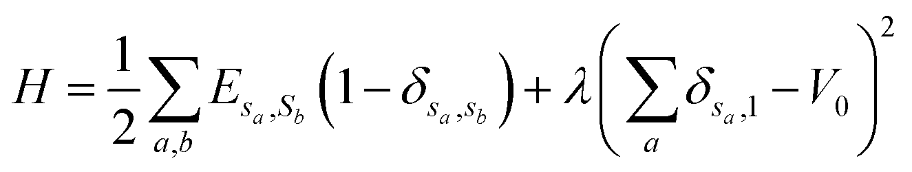 | (1) |
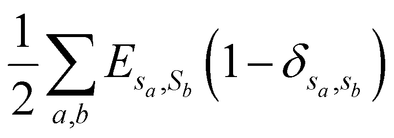 is the total surface energy of the system, sa is the spin of the selected lattice site, sb is the spin of the neighbour of the selected lattice site, Esa,sb is the surface energy, δsa,sb is the Kronecker delta function.
 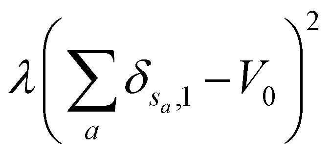 is the liquid volume energy, which is used to limit the fluctuation in liquid volume during the simulation. λ is the volume fluctuation coefficient, V0 is the liquid initial volume.
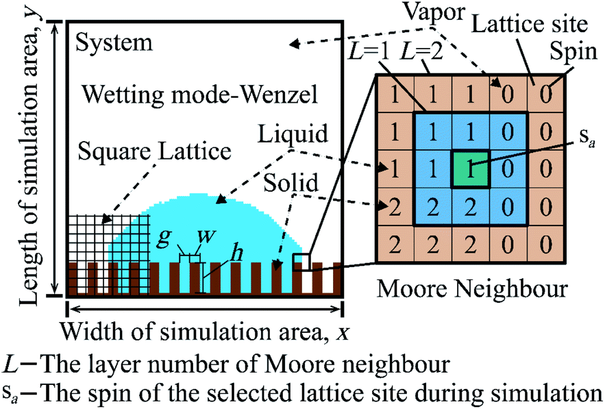 | ||
| Fig. 1 The wetting system of a droplet on a periodical grooved surface by using the cellular Potts model. Wetting mode of the system is Wenzel. x and y are the width and the length of the area of the simulation system. g, w, and h are interpillar distance, pillar width, and pillar height. In the part of Moore neighbour, L is the layer number of Moore neighbours. sa is the spin of the selected lattice site. sb is the spin of the Moore neighbour of the selected lattice site. 0, 1, and 2 represent vapor, liquid, and solid. | ||
Eqn (2) is the Metropolis algorithm, where k is the Boltzmann constant, T is the absolute temperature.
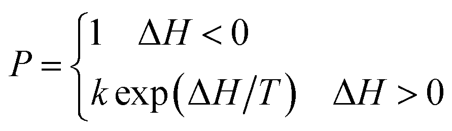 | (2) |
The CPM is adjusted as follows to accommodate the wettability simulation. (1) The flip of a spin only happens at the boundary of the liquid medium to ensure fluid continuity. (2) In Fig. 1, Moore neighbour layer (L) is the range of sb. The accuracy of the relationship between different media and the cost of computation time increase with an increase of L. L is set as 2 to not only guarantee less calculation time, but also to ensure the accuracy. (3) ΔH is only calculated in the sa Moore neighbour to reduce the consumption of calculation time. (4) Because the simulation parameters are dimensionless, k is set as 1. T is understood as the fluctuation parameter and not related to the thermodynamic temperature. (5) Square lattice is used to mesh the wetting system. Setting the spin of a lattice site as vapor (0), liquid (1), or solid (2). Set the initial state as Wenzel mode,24 as Fig. 1 shows.
Fig. 2 shows the flow diagram of obtaining the wetting mode transition diagram. In Fig. 2(a), surface energy, simulation, and structure parameters are set first. The system with different ḡ/![[h with combining macron]](https://www.rsc.org/images/entities/i_char_0068_0304.gif) is simulated by using the CPM. Dimensionless pillar height and interpillar distance ḡ are two variables. They are calculated by = h/R, ḡ = g/R, where h, g, R are pillar height, interpillar distance, and droplet radius. The Stable State (SS) post-processing or the Minimum Energy (ME) post-processing is used to export the result under the simulation of a single system. The SS selects the states of the last 1/5 of simulation time firstly and uses the average of the states as the result. The SS is used for comparison in this paper. It is because that a similar post-processing was used in ref. 24–26, and the average method is normally used to choose the result in the simulation by using the CPM. In ref. 24–26, states were chosen from the stable state after a long time of simulation. Some post-processing, which were not exhaustively described in those papers, were used to select the result from the states. The ME chooses the state with the minimum energy during the simulation process as a result. A critical transition point ḡcri should be recorded before adding Δ to . ḡcri is calculated by ḡcri = ḡLastC + Δḡ/2. ḡLastC is the ḡ of the system, whose simulation result is the last Cassie mode as ḡ increase. Finally, a transition diagram is obtained by connecting ḡLastC of each .
is simulated by using the CPM. Dimensionless pillar height and interpillar distance ḡ are two variables. They are calculated by = h/R, ḡ = g/R, where h, g, R are pillar height, interpillar distance, and droplet radius. The Stable State (SS) post-processing or the Minimum Energy (ME) post-processing is used to export the result under the simulation of a single system. The SS selects the states of the last 1/5 of simulation time firstly and uses the average of the states as the result. The SS is used for comparison in this paper. It is because that a similar post-processing was used in ref. 24–26, and the average method is normally used to choose the result in the simulation by using the CPM. In ref. 24–26, states were chosen from the stable state after a long time of simulation. Some post-processing, which were not exhaustively described in those papers, were used to select the result from the states. The ME chooses the state with the minimum energy during the simulation process as a result. A critical transition point ḡcri should be recorded before adding Δ to . ḡcri is calculated by ḡcri = ḡLastC + Δḡ/2. ḡLastC is the ḡ of the system, whose simulation result is the last Cassie mode as ḡ increase. Finally, a transition diagram is obtained by connecting ḡLastC of each .
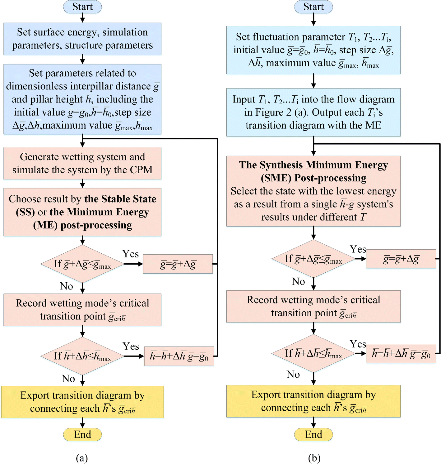 | ||
| Fig. 2 Flow diagram of obtaining the transition diagram. (a) Uses the Stable State (SS) post-processing and the Minimum Energy (ME) post-processing. (b) Uses the Synthesis Minimum Energy (SME) post-processing. | ||
In Figure (b), transition diagrams are simulated under T1, T2…, Ti firstly. Fig. 2(a) with the Minimum Energy (ME) post-processing is used as the flow diagram. The Synthesis Minimum Energy (SME) post-processing is used to export results. The SME records state with the minimum energy during the simulation process by various T, then it selects the state with the lowest energy from the records as the result. In all post-processing, each transition diagram is simulated five times and take the average diagram as the final result.
3. Results and discussion
The influence of the simulation time on wetting mode simulation is analyzed. An individual system is chosen as an example. The unit of simulation time is Monte Carlo Step (MCS). MCS is defined as the number of the trial of spin flips. MCS equals the total number of lattice sites in the simulated system. Surface energy, simulation, and structure parameters of the individual system simulation are set as follows. Liquid–vapor, solid–vapor, liquid–solid surface energy γlv, γsv, γls are 82, 82, and 130, where the intrinsic contact angle is 125.8°.25 This value is closed to the intrinsic contact angle of 126°, which was used to give an example in ref. 29. The surface energy is used as the Esa,sb in eqn (1). For example, when the sa is 1 and sb is 0, Esa,sb = E1,0 = γlv. 1 and 0 represent liquid and vapor. For the simulation parameters, the simulation time is set as 0.5 × 10⁴, 1.0 × 10⁴, 2.0 × 10⁴, 3.0 × 10⁴ MCSs to discuss the influence. Let T = 300 to ensure larger T have enough simulation time. λ = 25 to control the fluctuation rate of liquid volume within 0.50%, excluding the influence of volume fluctuation during the simulation. Width x and length y are 125 of the simulation area. For structure parameters, droplet radius R = 25. Since the droplet is very small in this paper, the influence of gravity can be neglected.29 Dimensionless pillar width![[w with combining macron]](https://www.rsc.org/images/entities/i_char_0077_0304.gif) = 0.16, pillar height = 0.40, and interpillar distance ḡ = 0.64. = w/R, where w is pillar width. Wetting modes of the results are clustered by visual inspection, but another possibility is to use an automatic unbiased approach (as clustering in ref. 30) and the latter possibility is probably the best for more complex systems.
= 0.16, pillar height = 0.40, and interpillar distance ḡ = 0.64. = w/R, where w is pillar width. Wetting modes of the results are clustered by visual inspection, but another possibility is to use an automatic unbiased approach (as clustering in ref. 30) and the latter possibility is probably the best for more complex systems.
The theoretical model is selected from Shahraz et al. in 2012.29 It is because that Shahraz et al. established a theoretical model of a two-dimensional droplet on the periodical grooved surface. In ref. 29, firstly, an energy equation was built to calculate the energy difference between a system consisting of a droplet on the surface and the surface without a droplet. Secondly, wetting modes were divided into Wenzel, Cassie, Mixed, and Epitaxial Cassie. The number of grooves beneath the drop was used as a parameter in each wetting mode. Finally, the energy difference of each wetting mode was calculated by the energy equation. The wetting mode, which had the lowest energy, was used as the result. Eqn (8)–(15) and (18)–(19) in ref. 29 are used in this paper. The theoretical model neglects the influence of gravity since the droplet is very small. The value of the droplet radius in ref. 29 is the same as this paper. The results of the theoretical model had compared with the experimental study under the same predictions and showed good accordance.
Fig. 3 reveals the change of energy variation rate of a system during the simulation process. Number 0 and 250 of the abscissa mean the start and the end sample of the simulation process. Result energy and wetting mode of the Stable State (SS) post-processing and the Minimum Energy (ME) post-processing are also showed. The simulation time is 3.0 × 10⁴ MCSs. Hf is the energy variation rate. Hf = [(Hr − H0)/H0] × 100%, Hr is the energy of the current system, H0 is the energy of the initial system. When Hf is negative, it means that the system has evolved into a state with a lower energy compared with the initial state. In Fig. 3, Hf decreases with an increase in the first few samples, and then a fluctuation is showed in the rest of the samples. It is because the purpose of the Metropolis algorithm is to evolve the simulated system into a stable state with lower energy. Hf = −5.8% of the ME result is lower than Hf = −2.0% of the SS result. The position of the ME result is in the middle of the simulation process. Wenzel mode of the ME result is the same as the theoretical prediction, while the wetting mode of the SS result is Cassie.
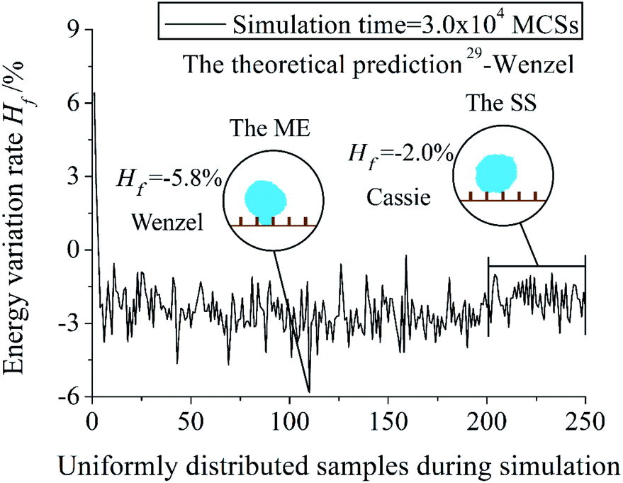 | ||
| Fig. 3 Energy variation of a single system during simulation. The dimensionless pillar width , pillar height , and interpillar distance ḡ of the system are 0.16, 0.40, and 0.64. Number 0 and 250 of the abscissa mean the start and the end sample of the simulation process. Post-processings of the Stable State (SS) and the Minimum Energy (ME) are used. | ||
In Fig. 4, the simulation of the system in Fig. 3 is extended to several simulation times. Positions of the Minimum Energy (ME) post-processing results in the simulation process are shown by the ring with the same number in the graph of energy variation during simulation. With an increase in the simulation time, the proportion of the stable state with lower energy in the total simulation process increases. Hf of the result of the ME post-processing decreases as the simulation time rises. It is because the simulation time is the total operation times of the Metropolis algorithm. The larger simulation time means the Metropolis algorithm gets more chances to evolve the system into a state with lower energy. The energy of the ME result is lower than the Stable State (SS) post-processing at the same simulation time. The Synthesis Minimum Energy (SME) post-processing selects the state with the minimum energy from all the ME results as a result. The increase in the simulation time will cause the deviating of the wetting mode of the SS results from the theoretical prediction at the simulation time = 2.0 × 10⁴ MCSs. Results of the ME and the SME are all Wenzel mode. The simulation time is set as 3.0 × 10⁴ MCSs to discuss the impact of T and post-processing. This setting can ensure the wetting systems in this paper have enough operation steps.
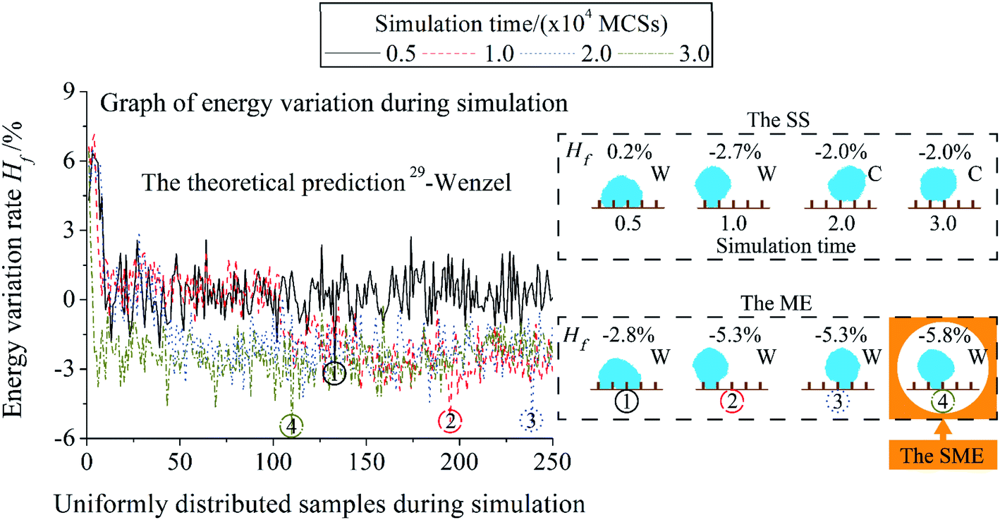 | ||
| Fig. 4 The influence of the simulation time on the simulation of a single system. The dimensionless pillar width , pillar height , and interpillar distance ḡ of the system are 0.16, 0.40, and 0.64. Black-solid, red-dash, blue-dot, and gold-dash-dot are used to represent the simulation time = 0.5, 1, 2, 3 × 10⁴ MCSs. Post-processings of the Stable State (SS), Minimum Energy (ME), and Synthesis Minimum Energy (SME) are used. Positions of the results of the ME in the simulation process are shown by the ring with the same number in the graph of energy variation during simulation. C represents Cassie mode and W represents Wenzel mode. | ||
For the discussion of the influence of T and post-processing, a system is selected as a research object at first. Dimensionless pillar width , pillar height and interpillar distance ḡ of the system are 0.16, 0.72, and 0.76. Fig. 5 shows the simulation results of the system as a function of T. T is set as 300, 325, 350, 375, and 400. The value of T is larger than the setting in ref. 21–23, 25, 27. It is because two Moore neighbour layers are used to calculate surface energy in this paper. |ΔH| in eqn (2) is larger than ref. 21–23, 25, 27 in the same flip of a site. A large T is set to adapt to the rise in |ΔH|. The simulation time is 3.0 × 10⁴ MCSs. Other simulation parameters are the same as the simulation in Fig. 3.
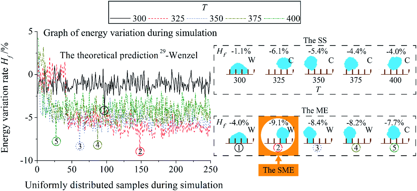 | ||
| Fig. 5 The influence of T on the simulation of a single system. The dimensionless pillar width , pillar height , and interpillar distance ḡ of the system are 0.16, 0.72, and 0.76. Black-solid, red-dash, blue-dot, gold-dash-dot, and green-dash-dot-dot are used to represent T = 300, 325, 350, 375, 400. Post-processings of the Stable State (SS), Minimum Energy (ME), and Synthesis Minimum Energy (SME) are used. Positions of the results of the ME in the simulation process are shown by the ring with the same number in the graph of energy variation during simulation. C represents Cassie mode and W represents Wenzel mode. | ||
In Fig. 5, for the energy of the result, a large T leads to a low result Hf of the Stable State (SS) post-processing and the Minimum Energy (ME) post-processing. Hf of the ME and the SS result gets its minimum value at T = 325. Thereafter, Hf of the SS and the ME result increase with an increase in T. For the wetting mode of the result, with a rise in T, the wetting mode of the SS result is different from the theoretical prediction at T = 325, while for the ME is at T = 400. Accept rate of the flip of a lattice site will go up in proportion to T when ΔH > 0. It can accelerate the speed of evolution and make the system evolve into a state with lower energy. However, too large T can evolve the system into a state with larger energy. Wenzel mode of the result of the Synthesis Minimum Energy (SME) post-processing is accordant to theory. An increase in T can induce the position of ME results close to the beginning of the simulation process.
Fig. 6 shows the influence of T on three different systems. Dimensionless pillar height of the system D, E, and F are 0.56, 0.72, and 0.88. Dimensionless pillar width , and interpillar distance ḡ of all the systems are 0.16 and 0.76. Each system is simulated five times and take the average as the result. In the same system, Hf of the result of the Minimum Energy (ME) post-processing is lower than the result of the Stable State (SS) post-processing. For the system D, the result Hf increases with an increase in T. While for the system E and F, a large T results in a reduction in the result Hf firstly. The system E gets its minimum Hf at T = 325. However, the system F is at T = 350. Thereafter, Hf of the system E and F increase as T increases. It is because the difference of pillar parameters causes the difference of ΔH during simulation. T needed to be changed to adapt to the ΔH change.
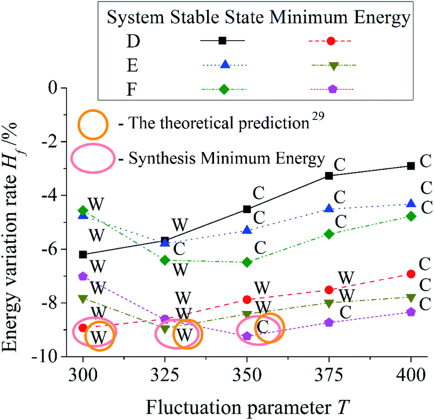 | ||
| Fig. 6 The influence of T on the simulation of three different systems. Three systems have different pillar height. Yellow-circular-ring and pink-oval-ring are used to point out the theoretical prediction and the result of the Syntheses Minimum Energy (SME) post-processing. C represents Cassie mode and W represents Wenzel mode. | ||
In Fig. 6, C represents Cassie mode and W represents Wenzel mode. For the Stable State (SS) post-processing, with an increase in T, the wetting modes of the system D and E deviate from the theoretical predictions at T = 350 and 325. However, the system F can't get the same wetting mode as theory before T = 350. For the Minimum Energy (ME) post-processing, the wetting modes of the system D and E deviate from the theoretical predictions at T = 400 with a rise in T. The ME shows more stability than the SS under the influence of T. Both the SS and the ME can't reach an agreement with the theoretical prediction in every T. In other words, a single value of T can't make every system get the accurate result due to the difference of pillar parameters. For the Synthesis Minimum Energy (SME) post-processing, the wetting modes of the results of the system D, E, and F are Wenzel, Wenzel, and Cassie mode. They are the same as theoretical predictions. It is because the SME selects the state with the lowest energy from the simulation results by various T. It satisfies the needs of various systems.
Fig. 7 and 8 show two transition diagram as a function of and ḡ. They are obtained by the flow diagram in Fig. 2. In Fig. 7, structure parameters are set as 0 = ḡ0 = 0.24, max = ḡmax = 0.96, Δ = Δḡ = 0.08. Other parameters are the same as the simulation in Fig. 5. In Fig. 8, surface energy γlv = 70, γsv = 25, γls = 50,24 simulation parameter T = 300, 350, 400, pillars structure 0 = 0.24, ḡ0 = 0, ḡmax = 0.64, = 0.64. The intrinsic contact angle is 110.9°. Other parameters are the same as Fig. 7. Mean standard deviation δm of the simulation result is calculated by  . The mean absolute error between the simulation result and theoretical prediction is ΔNm.
  . n is the total number of different in transition diagram, δi and ΔNi are the standard deviation and the absolute error of ḡLastC under a single .
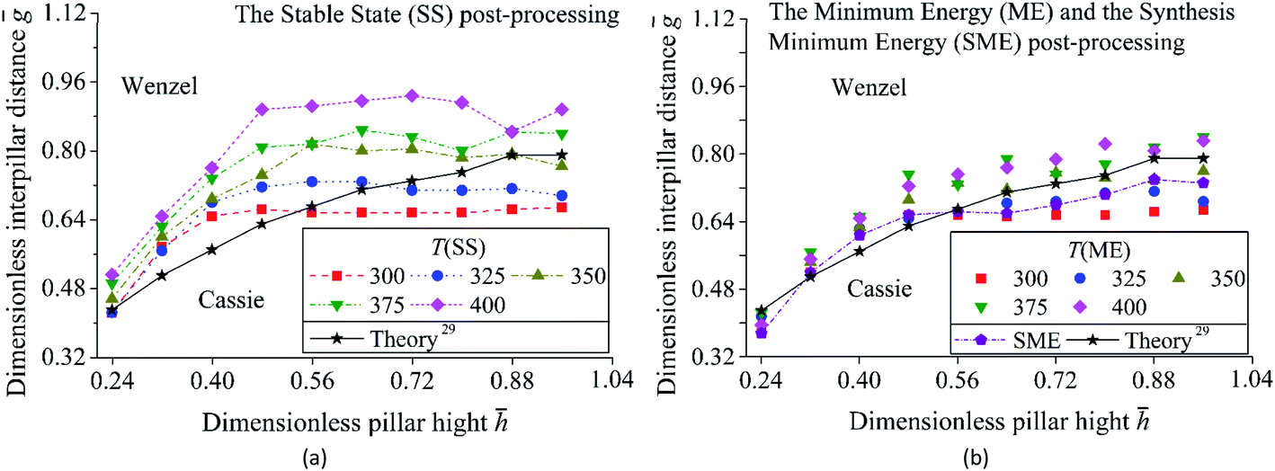 | ||
| Fig. 7 Transition diagram with an intrinsic contact angle 125.8°. (a) Uses the Stable State (SS) post-processing. (b) Uses the Minimum Energy (ME) post-processing and the Synthesis Minimum Energy (SME) post-processing. Above each transition curve is Wenzel mode, while the other is Cassie mode. | ||
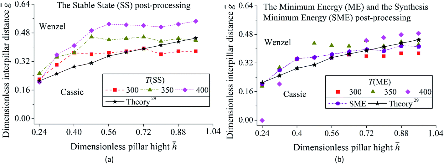 | ||
| Fig. 8 Transition diagram with an intrinsic contact angle 110.9°. (a) Uses the Stable State (SS) post-processing. (b) Uses the Minimum Energy (ME) post-processing and the Synthesis Minimum Energy (SME) post-processing. Above each transition curve is Wenzel mode, while the other is Cassie mode. | ||
In Fig. 7 and Table 1, wetting mode changes from Wenzel to Cassie with an increase in . However, with a rise in ḡ, wetting mode changes from Cassie to Wenzel. For the transition curve, a large leads to a high ḡ. The proportion of Cassie mode in the transition diagram and ΔNm show an increase with a rise in T. It is because that an increase in T leads to the wetting mode of the result changes from Wenzel to Cassie as Fig. 6 shows. The Minimum Energy (ME) post-processing and the Synthesis Minimum Energy (SME) post-processing decrease the proportion of Cassie state, δm, and ΔNm. For the ME, it gets the lowest ΔNm at T = 350 compare to other post-processings. For the SME, the result is the same as the results of the ME at T = 300, 325 when < 0.80 and a coupling of the results of the ME at T = 325, 350 when > 0.80. Its δm is less than and ΔNm is close to the result of the ME at T = 350.
| T | The Stable State (SS) post-processing | The Minimum Energy (ME) post-processing | The Synthesis Minimum Energy (SME) post-processing | |||
|---|---|---|---|---|---|---|
| δm | ΔNm | δm | ΔNm | δm | ΔNm | |
| 300 | 2.52 | 6.68 | 2.12 | 6.16 | 2.60 | 3.88 |
| 325 | 2.32 | 5.72 | 2.36 | 3.88 | ||
| 350 | 3.36 | 7.20 | 2.96 | 3.64 | ||
| 375 | 2.88 | 10.60 | 2.52 | 5.28 | ||
| 400 | 2.68 | 16.36 | 2.72 | 5.80 | ||
In Fig. 8 and Table 2, a surface with periodical pillars needs smaller ḡ to get Cassie mode compare to Fig. 7. It is because Fig. 8 has a smaller contact angle on the flat surface compare to Fig. 7. The Minimum Energy (ME) post-processing gets the best fitting to theory at T = 300, but not at T = 350 as Table 1 shows. The Synthesis Minimum Energy (SME) post-processing gets the lowest ΔNm compare to other post-processings. As Tables 1 and 2 show, ME/SME can effectively improve the accuracy of wetting modes simulation. The ME can't guarantee that each system gets a good agreement with theory under a single T. However, the SME shows good ability in promoting the accuracy of the simulation of various systems. The mean relative error of the contact angle between simulation and theory is 4–6° in all simulations.
| T | The Stable State (SS) post-processing | The Minimum Energy (ME) post-processing | The Synthesis Minimum Energy (SME) post-processing | |||
|---|---|---|---|---|---|---|
| δm | ΔNm | δm | ΔNm | δm | ΔNm | |
| 300 | 2.44 | 3.92 | 1.92 | 3.44 | 2.96 | 2.44 |
| 350 | 2.16 | 6.48 | 1.76 | 4.56 | ||
| 400 | 3.60 | 11.68 | 2.00 | 5.68 | ||
There is still has a discrepancy between the theory and simulation after used the Synthesis Minimum Energy (SME) post-processing in Fig. 7 and 8. To discuss the reason for the discrepancy, the result in Fig. 7 is reprocessed by the SME with different groups of values of T. In a group of T, the range and step size are used to represent the values of T. The mean absolute error ΔNm between the simulation result and the theoretical prediction of the reprocessing is shown in Table 3. In Table 3, when the minimum of the range and step size of T are 300 and 25, the ΔNm decreases with the increase of maximum. The ΔNm of the range with the maximum 375 and 400 is the same. For the range with the minimum 300 and maximum 400, the decrease in step size will cause a decrease in the ΔNm. While for the range with the minimum 300 and maximum 350, the value between the ΔNm with step size 25 and 50 is close. It is because that the wetting systems, which have different pillar height and interpillar distance in Fig. 7, need different values of T to get a lower energy. The more lower energy the system gets, the more the system closes to the state with the global lowest energy. The increase in the range and the decrease in the step size of T will enable more wetting systems to get closer to the global lowest energy, so the simulation accuracy of the SME will be improved. But the increase in the number of values of T will cause an increase in the total consumption of calculation time of the transition diagram and a decrease in the ability of accuracy improvement. For example, with the same minimum 300 of the range of T, ΔNm changes from 5.03 × 10⁻² to 4.04 × 10⁻² when the maximum changes from 325 to 350, while ΔNm only changes from 4.04 × 10⁻² to 3.88 × 10⁻² when the maximum changes from 350 to 375.
| Range of T | ΔNm | |||
|---|---|---|---|---|
| Step size of T | ||||
| Minimum | Maximum | 25 | 50 | 100 |
| 300 | 325 | 5.03 | Non | Non |
| 300 | 350 | 4.04 | 3.92 | Non |
| 300 | 375 | 3.88 | Non | Non |
| 300 | 400 | 3.88 | 4.16 | 5.60 |
At the same time, the range of T should be set appropriately. As Table 3 shows, after eliminating the maximum 400, the total consumption of calculation time will be decreased and the lowest ΔNm will be not changed. The reason why the ΔNm of the range with the maximum 375 and 400 is the same is because that the energy of the results is much larger than the global lowest energy when T = 400. Besides, a small step size should be combined with a large range of T to show a good improvement in the accuracy. For the result of the SME in Fig. 7, the discrepancy between the theory and simulation can be decreased by decreasing the step size of T. But this movement will cause less improvement in the accuracy and a large total consumption of calculation time of the transition diagram.
For the use of the Synthesis Minimum Energy (SME) on the simulations of other functional surfaces such as 3D periodical grooved surface by the CPM, the operational process is as bellow. Firstly, some test systems, which have different properties like structure parameters and surface energy, are chosen for setting the simulation parameters. Secondly, the simulation time should be set as enough value to guarantee the test systems have enough operation steps, as Fig. 4 shows. Thirdly, a group of values of T with the presupposed range and step size is used for the simulation test. The range of T will be reset during the test to make sure the test systems get the relatively lower energy. Fourthly, the step size can be decreased to increase the accuracy. The range of T can be decreased to eliminate the values of T, which do not influence the accuracy. The range and step size of T should be set based on the consideration of accuracy and total consumption of calculation time. Finally, all the systems can be simulated by the values of T, which were set in the previous step, to get the final result by the SME.
4. Conclusions
Wetting mode transition diagrams were simulated by using the Cellular Potts Model (CPM). The Synthesis Minimum Energy (SME) post-processing was proposed to improve the accuracy of the wetting mode simulation by using the CPM. The conclusions are as follows.(1) The Synthesis Minimum Energy (SME) post-processing can decrease the influence of T and promote the accuracy of wetting mode simulation in various systems. It is because the SME records the state with the minimum energy during the simulation process under various T firstly, and selects the state with the lowest energy from the records as the result.
(2) For the values of T used in the SME, the accuracy of the result of the SME increases as the range of T increases and the step size of T decreases. The increase in the number of values of T will also cause an increase in the total consumption of calculation time and a decrease in the ability of accuracy improvement. For the use of the SME, the range and step size of T should be set based on the consideration of accuracy and total consumption of calculation time.
Conflicts of interest
There are no conflicts to declare.Acknowledgements
This paper was supported by The State Key Program of National Natural Science Foundation of China (U1637206), Foundation for Innovative Research Groups of the National Natural Science Foundation of China (51521003), and Shanghai Sailing Program (20YF1417200).References
- J. Bico, C. Marzolin and D. Quéré, Europhys. Lett., 1999, 47, 220–226 CrossRef CAS.
- L. Ionov and A. Synytska, Phys. Chem. Chem. Phys., 2012, 14, 10497–10502 RSC.
- H. Zhang, Y. Q. Li, Y. G. Xu, Z. X. Lu, L. H. Chen, L. L. Huang and M. Z. Fan, Phys. Chem. Chem. Phys., 2016, 18, 28297–28306 RSC.
- Y. Zheng, H. Bai, Z. Huang, X. Tian, F. Nie, Y. Zhao, J. Zhai and L. Jiang, Nature, 2010, 463, 640–643 CrossRef CAS.
- E. Kang, G. S. Jeong, Y. Y. Choi, K. H. Lee, A. Khademhosseini and S. H. Lee, Nat. Mater., 2011, 10, 877–883 CrossRef CAS.
- H. Chen, P. Zhang, L. Zhang, H. Liu, Y. Jiang, D. Zhang, Z. Han and L. Jiang, Nature, 2016, 532, 85–89 CrossRef CAS.
- D. L. Tian, X. F. Zhang, X. Wang, J. Zhai and L. Jiang, Phys. Chem. Chem. Phys., 2011, 13, 14606–14610 RSC.
- J. Guo, F. C. Yang and Z. G. Guo, J. Colloid Interface Sci., 2016, 466, 36–43 CrossRef CAS.
- G. N. Ren, Y. M. Song, X. M. Li, Y. L. Zhou, Z. Z. Zhang and X. T. Zhu, Appl. Surf. Sci., 2017, 428, 520–525 CrossRef.
- X. Y. Gao, G. Wen and Z. G. Guo, New J. Chem., 2019, 43, 16656–16663 RSC.
- Y. B. Li, B. C. Li, X. Zhao, N. Tian and J. P. Zhang, ACS Appl. Mater. Interfaces, 2018, 10, 39391–39399 CrossRef CAS.
- N. A. Patankar, Langmuir, 2004, 20, 8209–8213 CrossRef CAS.
- T. Liu, Y. Li, X. Li and W. Sun, J. Phys. Chem. C, 2017, 121, 9802–9814 CrossRef CAS.
- S. Xiao, Z. Zhang and J. He, Phys. Chem. Chem. Phys., 2018, 20, 24759–24767 RSC.
- T. Li, M. Li, J. Wang, J. Li, Y. Duan and H. Li, Phys. Chem. Chem. Phys., 2018, 20, 24750–24758 RSC.
- E. S. Savoy and F. A. Escobedo, Langmuir, 2012, 28, 16080–16090 CrossRef CAS.
- S. Khan and J. K. Singh, Mol. Simulat., 2014, 40, 458–468 CrossRef CAS.
- A. Giacomello, M. Chinappi, S. Meloni and C. M. Casciola, Phys. Rev. Lett., 2012, 109, 226102 CrossRef.
- E. Lisi, M. Amabili, S. Meloni, A. Giacomello and C. M. Casciola, ACS Nano, 2018, 12, 359–367 CrossRef CAS.
- W. Ren, Langmuir, 2014, 30, 2879–2885 CrossRef CAS.
- L. R. de Oliveira, D. M. Lopes, S. M. M. Ramos and J. C. M. Mombach, Soft Matter, 2011, 7, 3763–3765 RSC.
- D. M. Lopes, S. M. M. Ramos, L. R. de Oliveira and J. C. M. Mombach, RSC Adv., 2013, 3, 24530–24534 RSC.
- V. Mortazavi, R. M. D'Souza and M. Nosonovsky, Phys. Chem. Chem. Phys., 2013, 15, 2749–2756 RSC.
- H. C. M. Fernandes, M. H. Vainstein and C. Brito, Langmuir, 2015, 31, 7652–7659 CrossRef CAS.
- D. M. Lopes and J. C. M. Mombach, Braz. J. Phys., 2017, 47, 672–677 CrossRef.
- M. Silvestrini and C. Brito, Langmuir, 2017, 33, 12535–12545 CrossRef CAS.
- V. Mortazavi and M. M. Khonsari, Tribol. Int., 2018, 123, 61–70 CrossRef.
- F. Graner and J. A. Glazier, Phys. Rev. Lett., 1992, 69, 2013–2016 CrossRef CAS.
- A. Shahraz, A. Borhan and K. A. Fichthorn, Langmuir, 2012, 28, 14227–14237 CrossRef CAS.
- A. Giacomello, S. Meloni, M. Chinappi and C. M. Casciola, Langmuir, 2012, 28, 10764–10772 CrossRef CAS.
| This journal is © The Royal Society of Chemistry 2021 |