
 Open Access Article
 This Open Access Article is licensed under a Creative Commons Attribution-Non Commercial 3.0 Unported Licence
The viscoelasticity of adherent cells follows a single power-law with distinct local variations within a single cell and across cell lines
Juan G.
Sanchez
 ,
Francisco M.
Espinosa
,
Ruben
Miguez
and
Ricardo
Garcia
*
,
Francisco M.
Espinosa
,
Ruben
Miguez
and
Ricardo
Garcia
*
Instituto de Ciencia de Materiales de Madrid, CSIC, c/Sor Juana Inés de la Cruz 3, 28049 Madrid, Spain. E-mail: r.garcia@csic.es
First published on 28th September 2021
Abstract
AFM-based force–distance curves are commonly used to characterize the nanomechanical properties of live cells. The transformation of these curves into nanomechanical properties requires the development of contact mechanics models. Spatially-resolved force–distance curves involving 1 to 2 μm deformations were obtained on HeLa and NIH 3T3 (fibroblast) cells. An elastic and two viscoelastic models were used to describe the experimental force–distance curves. The best agreement was obtained by applying a contact mechanics model that accounts for the geometry of the contact and the finite-thickness of the cell and assumes a single power-law dependence with time. Our findings show the shortcomings of elastic and semi-infinite viscoelastic models to characterize the mechanical response of a mammalian cell under micrometer-scale deformations. The parameters of the 3D power-law viscoelastic model, compressive modulus and fluidity exponent showed local variations within a single cell and across the two cell lines. The corresponding nanomechanical maps revealed structures that were not visible in the AFM topographic maps.
The last 15 years have seen the consolidation of a live cell as a system that responds to mechanical interactions and biochemical processes. This realization emphasises the close relationship among mechanical forces, cell shape and physiology.1–5 The field of mechanobiology is stimulating the development of sensitive, quantitative and high-spatial resolution methods based on mechanical probes and interactions.6–13 Atomic force microscopy (AFM) is playing a significant role in advancing of our understanding of the mechanical response of a live cell.6,14–16 High-spatial resolution imaging, force spectroscopy capabilities, non-invasiveness, nanomechanical mapping and operation in biological buffers are features exploited to advance our understanding of the properties at the single cell level.
The intrinsic heterogeneity of a cell or the lack of a generally accepted contact mechanics model to fit the data and the changes of a cell (shape) during a measurement complicate the interpretation and/or standardization of AFM measurements on cells. Commonly, Sneddon expressions17 are used to fit AFM-based force–distance curves (FDCs). However, the finite-thickness of a mammalian cell might preclude the use of Sneddon expressions to determine the elastic modulus of a cell (see below).16 The above issue has led to a paradoxical situation. At a qualitative level, AFM measurements show a high degree of reproducibility. The observation that a cancer cell is softer than a non-malignant cell has been reproduced by many groups.18–22 Similarly, AFM data have firmly established that drug inhibitors of actin polymerization reduce the Young's modulus.23,24,54 On the other hand, the values of the Young's modulus measured on cells of the same line might differ by 5-fold.25 Even the methodology applied to determine the Young's modulus of a cell might be questionable. After all, a large body of experimental data has shown conclusive evidence about the viscoelastic response of a mammalian cell.7,16,24,26–31
Here we aim to clarify the complex nanomechanical response of a mammalian cell as determined from AFM force–distance curves on three aspects. First, by showing that the intrinsic viscoelastic response of a cell is preserved in a force–distance curve measurement. Second, by implementing an analytical force reconstruction model that provides a faithful representation of the mechanical state of a live cell. This model which is called 3D power-law viscoelasticity (3D-PLR) hereafter expresses the dependence of the force exerted on a cell by a conical tip in terms of the indentation, the cell's thickness, the compressive modulus at an arbitrary time t0 and the fluidity exponent. Third, by showing that the compressive modulus and the fluidity exponent characterize the spatially-dependent nanomechanical response of a cell within the same cell line and across different cell lines. Specifically, we show that cytoplasmatic regions have more liquid-like properties than nuclear regions. By performing experiments on fibroblasts (NIH 3T3) and HeLa cells, we demonstrate that the finite-thickness of a cell must be accounted for to determine mechanical parameters from force–distance curves. In summary, our results underline the robustness of the compressive modulus and the fluidity exponent to characterize the mechanical state of a mammalian cell under micrometer deformations performed at low frequencies.
Results and discussion
We analyse separately the role of the contact mechanics models, cell's finite-thickness and the spatial heterogeneity of the nanomechanical parameters extracted from force–distance curves.Theory and contact mechanics models to determine force–distance curves
We have considered three contact mechanics models to determine the nanomechanical parameters extracted from a force–distance curve. An elastic model that incorporates bottom effect corrections.32 A linear viscoelastic model which accounts for the deformation history (approach versus retraction) and incorporates bottom effect corrections.33 Finally, we have implemented a power-law viscoelastic model that incorporates both the deformation history and bottom effect corrections.31A 3D elastic model for a finite-thickness cell
Pyramidal tips are commonly used to perform AFM experiments on cells. A conical tip might offer the closest axisymmetric geometry to model a pyramidal tip. Sneddon derived an expression to determine the force exerted by a conical tip on a semi-infinite elastic sample as a function of the indentation I, the semi-angle of the cone θ, the Poisson's ratio ν and the effective Young's modulus E of the cell17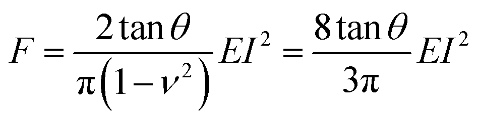 | (1) |
Starting from the above expression, Garcia and Garcia developed an analytical expression to determine the force exerted by a conical tip on a cell of thickness h that rests on a rigid solid support,34
 | (2) |
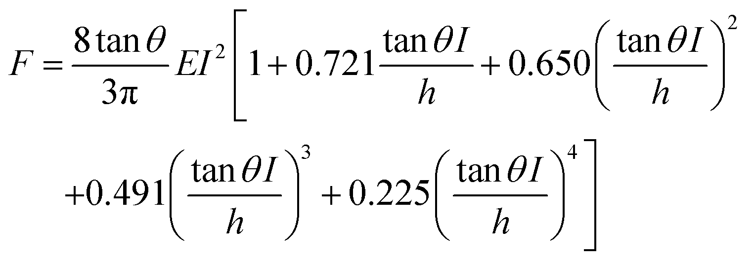
Eqn (2) enables to determine the Young's modulus of a cell without the influence of the rigid support. In this context, a polynomial expansion in terms of (I/h)n is commonly called bottom-effect correction.8,16
A 3D linear viscoelastic model for a finite-thickness cell
This model combines the standard Kelvin–Voigt model which consists in a 1D elastic spring in parallel to a 1D viscous element (dashpot) with the geometry of the deformation25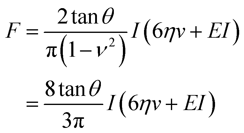 | (3) |
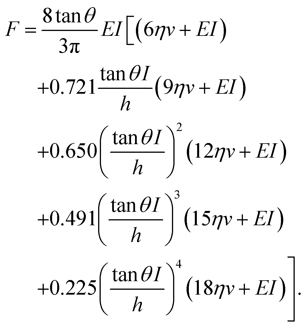 | (4) |
A 3D power law viscoelastic model for a finite-thickness cell
Kollmannsberger and Fabry proposed that the mechanical response of a cell to an external force might be explained in terms of the viscoelastic properties of soft glassy materials.27,28 This model postulates that the creep compliance follows a power law dependence on time (J = J0tγ). This response might involve a broad distribution of relaxation times. This insight opened the development and/or implementation of power-law models to fit the FDCs measured by AFM.31,34–43 We have considered that the modulus of a cell follows a single power-law dependence with time characterized by two parameters, E0 and γ,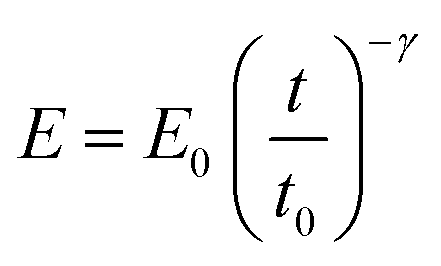 | (5) |
E 0 is defined as the compressive modulus of the material at time t0 and γ is called the fluidity exponent. In a previous publication32 we defined E0 as the Young's modulus at a time of 1 s. However, we prefer to use the term compressive modulus to avoid the identification with an elastic modulus. A value of the fluidity exponent γ = 0 indicates an elastic solid while γ = 1 indicates a viscous liquid. Based on the above power-law equation, Garcia, Guerrero and Garcia31 deduced an analytical expression to determine the force as a function of indentation. The model accounts for the geometry of the contact, the finite-thickness of a cell and the history of the deformation. The analytical force expression was deduced in several steps. First, the force was deduced for a semi-infinite, incompressible (ν = 0.5) power-law viscoelastic material,
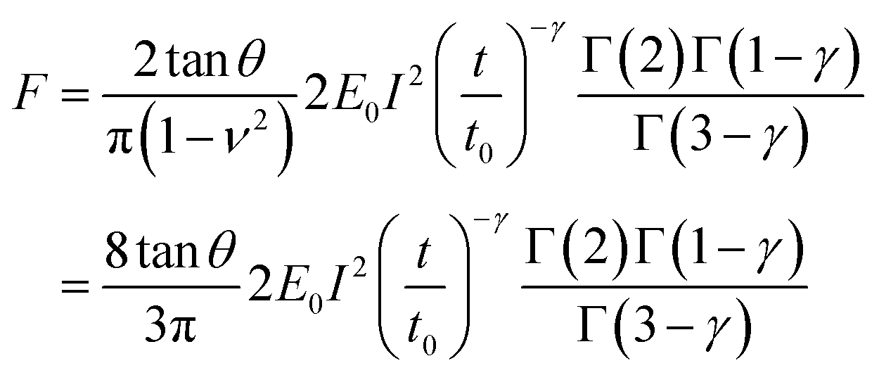 | (6) |
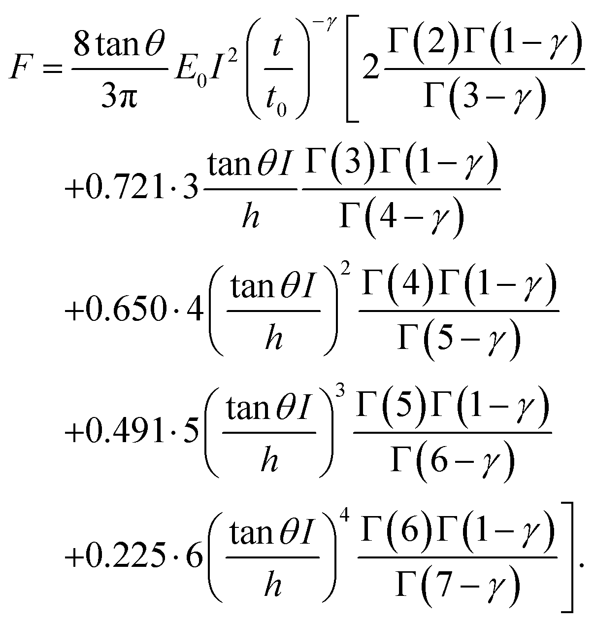 | (7) |
Third, we applied Ting's procedure44 to determine the contact area during the tip's withdrawal. A force–distance curve measurement involves the acquisition of the force as the tip approaches the cell and withdraws from it. The viscoelastic response implies the existence of a time shift between the maximum force and the maximum indentation. To determine the force applied to a viscous material during the withdrawal we applied the following transformations
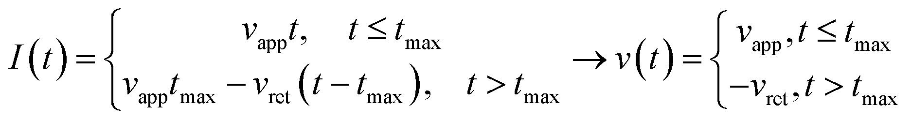 | (8) |
 | (9) |
Experimental force–distance curves
To access the cell's nanomechanical properties we have used force–distance curves generated using a triangular waveform. An FDC can be directly compared to a theory without making any implicit assumption on the experimental data. The comparison provides a direct assessment of the validity of the theory to describe the data. To the best of our knowledge, this is a distinct feature with respect other methods aimed to measure viscoelastic properties.The AFM data were used to plot the force as a function of time or indentation. The relevant AFM observations were the cantilever deflection, the z-piezo displacement and the displacement at which the tip contacts the cell surface. The distance was considered negative when the tip is indenting the cell. The indentation was stopped when the force reached a threshold level of 3 nN.
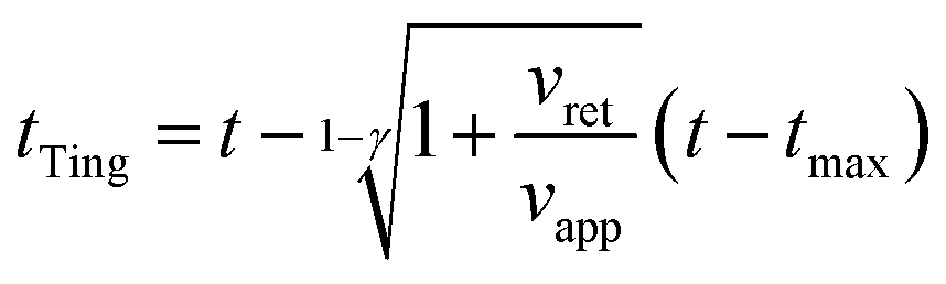
Fig. 1a shows a sequence of 5 FDCs obtained on the same spot of a HeLa cell. The thick line is the mean value. The triangular waveform and the dependence of the z-tip deflection with time are shown in Fig. 1b. Fig. 1c shows a compact representation of the FDC as a function of indentation.
 | ||
| Fig. 1 Force–distance curves obtained on HeLa cells. (a) The force is represented versus the z-piezo displacement. This is the most common representation of a FDC. Five successive curves are shown (grey). The thick curve shows the mean value (b). Mean curve plotted as a function of time. The right axis shows the indentation signal. (c) Compact representation of a FDC. The force is represented as a function of the tip's indention on the cell. Curves obtained over a region on top of the nucleus. Parameters: Fpeak = 3 nN; v = 10 μm s−1 (fm ≈ 3.5 Hz); k = 0.075 N m−1; FDC acquisition rate 500 points per μm; h = 5 μm. | ||
The acquisition of a FDC implies the selection of a velocity or a modulation frequency. The velocity is easily determined for a triangular waveform; however, the contact time or its inverse (fm = 1/tc) provides more information on the cell's nanomechanical response. Indeed, the nanomechanical response of a live cell does depend on the tip's modulation frequency or velocity.10,24 To simplify the discussion and interpretation of the experimental data, we have chosen a velocity of 10 μm s−1 (tc = 0.27 s, fm = 3.7 Hz). A velocity of 10 μm s−1 provides a good compromise between moderately quick data acquisition speed and yet the measured parameters are representative of cell's response in the 0.5–5 Hz range.
Elastic versus viscoelastic descriptions of a live cell
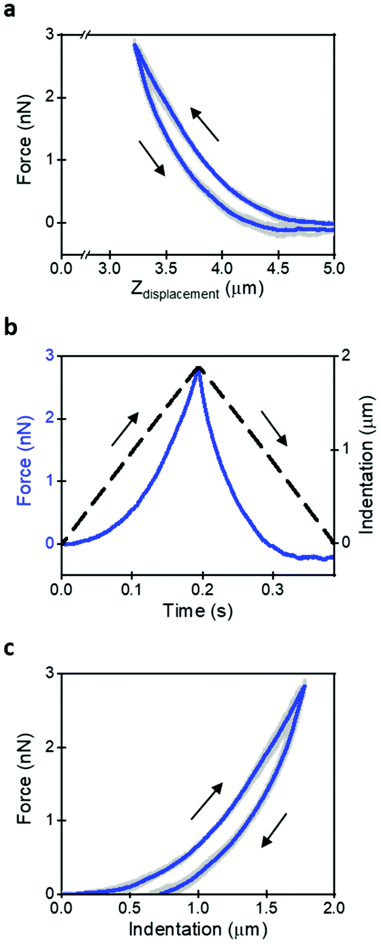
The implications derived from the intrinsic viscoelastic nature of a mammalian cell have yet to reach a general acceptance. For example, a large number of AFM-based studies are based on the use of elastic contact mechanics models.46 An FDC reveals that the approaching and retraction sections of the force–distance curve do not overlap. The hysteresis implies the existence of energy dissipative processes inside a cell.45,47,48 It must be noted that creep and other non-linearities in the z-piezo displacement might also introduce hysteresis in an FDC. Those effects must be removed before processing the data to determine the genuine viscoelastic parameters of a cell.Fig. 2 shows some FDCs obtained on HeLa and NIH 3T3 cells. The 3D elastic model leads to two Young's modulus values depending on the section of the FDC used for the fitting (approach or retraction). For both cell lines, the modulus obtained during the retraction is about 3 times higher than the one obtained during the approach. The existence of two values should question the use of elastic models. The AFM community has resorted to present the data obtained during the approach without providing a proper justification.
 | ||
| Fig. 2 Comparison experiment and elastic model expressions. (a) HeLa cell. (b) NIH 3T3 cells. Continuous curve (experiment); dotted and dashed lines are the results from the analytical model. Parameters of the FDCs: Fpeak = 3 nN, FDC acquisition rate of 500 points per μm; k (HeLa) = 0.075 N m−1, k (NIH 3T3) = 0.133 N m−1; h (HeLa) = 4.5 μm, h (NIH 3T3) = 6.8 μm. | ||
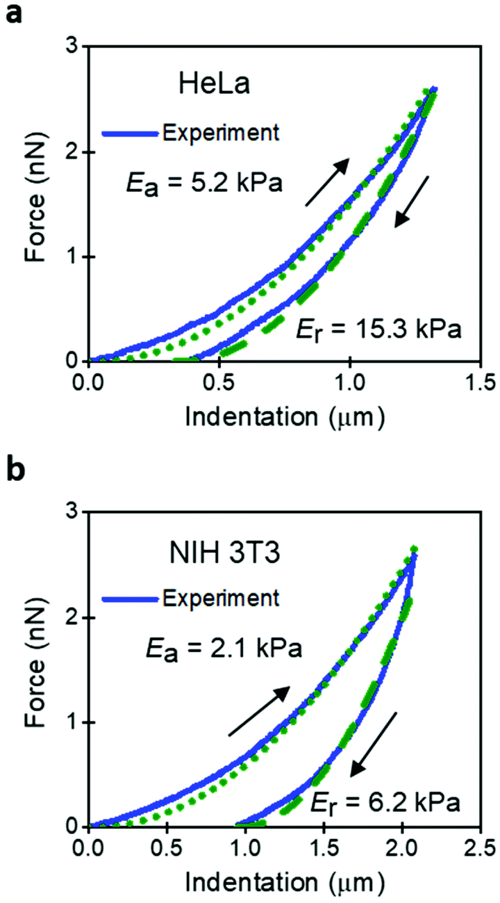
Fig. 3 compares the experimental FDCs to the force expressions of the viscoelastic models. The 3D linear viscoelastic model (3D-KV) provides an excellent fitting to the approach section for both cell lines. However, it shows a step discontinuity at the turning point which prevents a good fitting of the retraction section of the FDC. This artefact is associated with the change in the sign of the velocity. Therefore, we do not recommend the use of the 3D-KV model if the FDC was generated using a triangular waveform. On the other hand, the 3D-PLR model does provide a good fitting for the both sections (approach and retraction). This agreement cannot be considered fortuitous because the model has just two parameters. For this reason, in the next sections, the 3D-PLR model will be used to describe the nanomechanical response of live cells.
 | ||
| Fig. 3 Comparison of experiment and analytical viscoelastic models. (a) 3D power-law viscoelastic model. (b) 3D-Kelvin–Voigt. Parameters of the FDCs as in Fig. 2. | ||
From the above analysis, we conclude that the nanomechanical response of a cell cannot and should not be described by an elastic model. This conclusion comes from three reasons. First, the values Ea and Er are very different. Second, the values of the Young's modulus do not coincide with the effective modulus provided by a viscoelastic model. Third, the FDCs show hysteresis and the existence of energy dissipative processes.
It is not straightforward to understand 3D power-law rheology in terms of physical concepts. However, we consider that different effects such as poroelasticity50 and the hydrodynamic drag of cell's organelles13 contribute to 3D power law rheology.
Influence of the elastic modulus on the solid support
Commonly AFM experiments are performed on cells cultured on rigid supports such as Petri dish or glass. The Young's modulus of those materials (10–100 GPa) is several orders of magnitude higher than the effective modulus of a cell (0.2–10 kPa). The finite-thickness of a cell, its very low effective modulus and the application of relatively large indentations (1–2 μm) imply that the stiffness of the rigid support will increase the force exerted by the tip with respect to a semi-infinite material of identical mechanical properties. This is an unavoidable effect. However, it can be corrected using force–distance equations deduced with a bottom-effect correction model.To illustrate the type of numerical errors associated with the Young's modulus of the rigid support, we have compared the compressive modulus and the fluidity coefficient measured on several HeLa and NIH 3T3 cells. For HeLa cells (Fig. 4a), the box plots show mean values, respectively, 2348 Pa (semi-infinite) and 2219 Pa (finite). For NIH 3T3 cells (Fig. 4b), we obtained 574 Pa (semi-infinite) and 533 Pa (finite). This is a semi-infinite viscoelastic model overestimates the compressive modulus by about 6–10%. On the other hand, the fluidity exponent (0.29) seems to be unaffected by the stiffness of the solid support. A similar trend is obtained on NIH 3T3 cells (Fig. 4c). The same trend, semi-infinite models overestimate the modulus of cells, was observed when elastic expressions were used. Table 1 shows a summary of all the measurements.
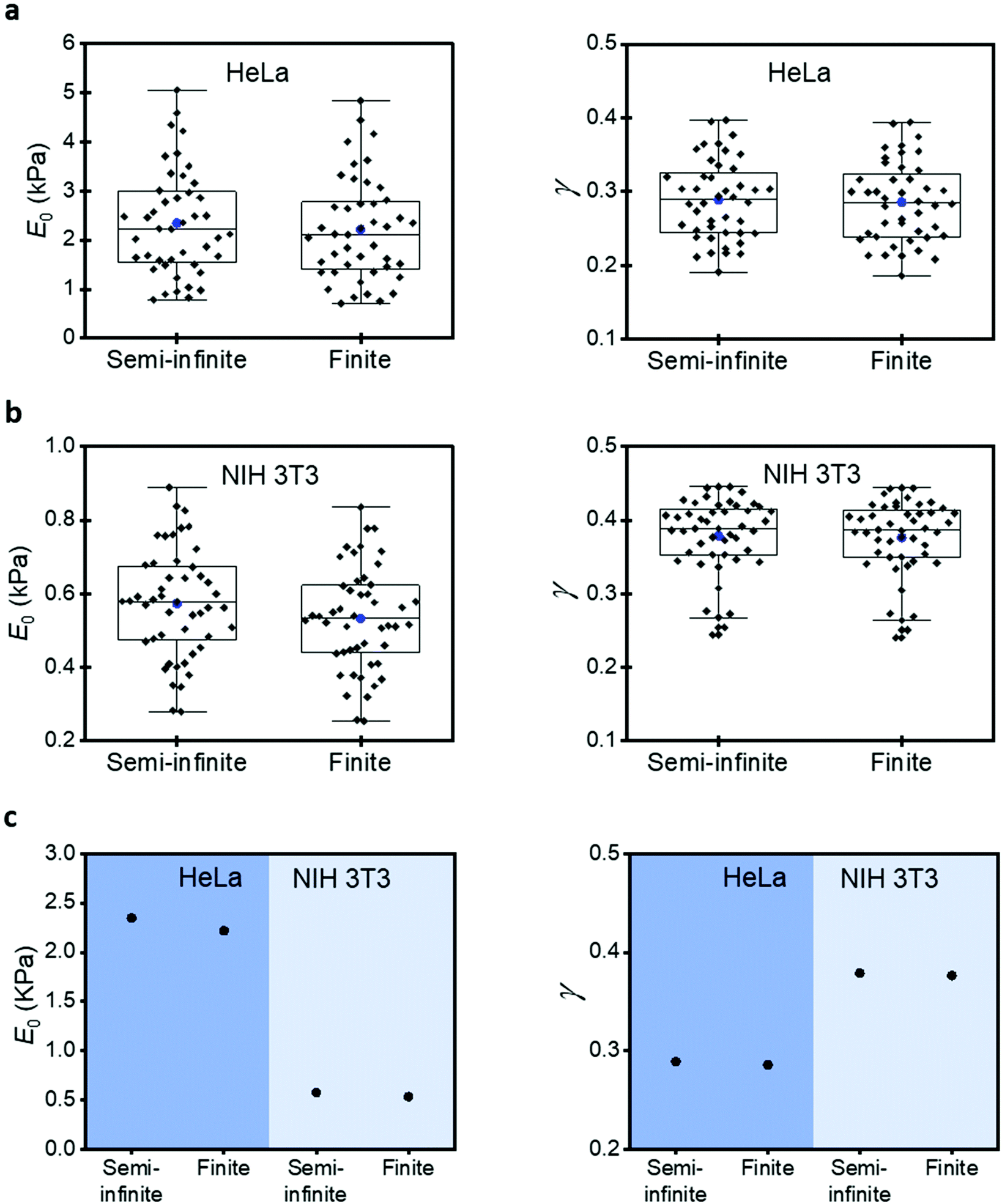 | ||
| Fig. 4 Effect of the rigid support on the compressive modulus and fluidity exponent values. (a) HeLa cells. (b) Fibroblasts (NIH 3T3). (c) Mean values for HeLa and NIH 3T3 cells. Semi-infinite and finite indicate the thickness of the material used in the theory (h (HeLa) ≈ 5 μm, h(NIH 3T3) ≈ 7 μm). FDCs obtained by applying the force on a plasma membrane region located above the nucleus. | ||
| Cell | Thickness | Elastic model | Single power law model | ||||
|---|---|---|---|---|---|---|---|
| E (Pa) | E 0 (Pa) | γ | |||||
| NIH3T3 | Semi-infinite | 2254 | 2225 | 574 | 484 | 0.38 | 0.42 |
| Finite | 2092 | 1977 | 533 | 431 | 0.38 | 0.41 | |
| HeLa | Semi-infinite | 7320 | 5769 | 2348 | 1539 | 0.29 | 0.33 |
| Finite | 6836 | 5293 | 2219 | 1416 | 0.29 | 0.32 | |
| Nucleus | Cytoplasm | Nucleus | Cytoplasm | Nucleus | Cytoplasm | ||
Mechanical differences between HeLa and NIH 3T3 cells
A mammalian cell is made of a plasma membrane that encapsulates a variety of solid elements (single proteins, RNA–protein complexes, filaments, nucleus, and organelles) immersed in an aqueous medium (cytosol). This structure gives rise to a high mechanical heterogeneity within a cell and across different cell lines.Fig. 5 compares the parameters of the 3D power-law rheology model measured on NIH 3T3 fibroblasts and HeLa cells. The compressive modulus of the HeLa cells is significantly higher (about five-fold). For example, the mean values over the nuclear region are, respectively, 2219 and 533 Pa. Similar differences are observed for the cytoplasmatic regions (1416 versus 431 Pa). The fluidity exponent also reflects the differences between HeLa and NIH 3T3 cells. Higher fluidity exponents are found on NIH 3T3 cells. The mean values over the nuclear regions are, respectively, of 0.38 (NIH 3T3) and 0.29 (HeLa) Interestingly, the differences observed between HeLa and NIH 3T3 cells are larger than the differences measured among the regions of the same cell lines. Overall, HeLa cells are stiffer and less viscous than NIH 3T3 cells.
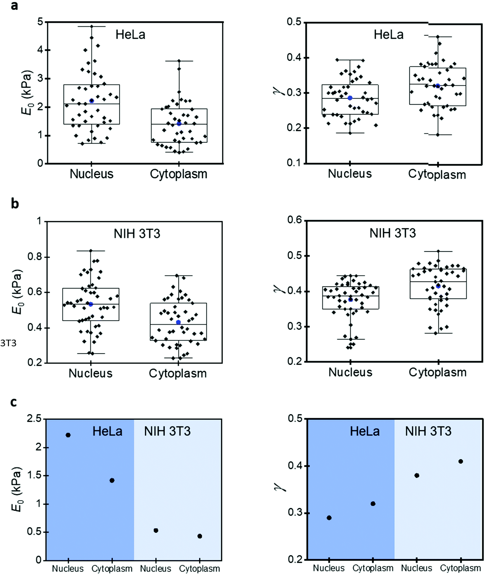 | ||
| Fig. 5 Compressive and fluidity exponent values over nuclear and cytoplasmic regions. (a) Box plot from HeLa cells. (b) Box plot from NIH 3T3 cells. (c) Mean values of the compressive modulus and fluidity exponent for different cell lines. | ||
Nucleus versus cytoplasm
Let's discuss first the effect of the cell surface curvature on the nanomechanical data. Side view confocal microscopy images (not shown) show that over the central region of the nucleus, the cell surface is perpendicular to the cantilever. Thus, all the force exerted by the tip is used to compress the cell. This is no longer the case for experiments performed on the cytoplasm. The force generating the cell's deformation is Ftip cos![[thin space (1/6-em)]](https://www.rsc.org/images/entities/char_2009.gif) α. The angles α (average value) are 37° and 10° for HeLa and NIH 3T3 cells, respectively.
α. The angles α (average value) are 37° and 10° for HeLa and NIH 3T3 cells, respectively.
Fig. 5 also shows the differences between the nuclear and cytoplasmatic regions. Those differences were reported previously by measuring variations of Young's modulus between the nuclear and cytoplasmic regions. The Young's modulus values measured over the nucleus are higher than those measured on the cytoplasm.13,49 However, we showed above the limitations of elastic models to describe the deformation of a mammalian cell, for that reason, we have revisited this problem by applying the 3D power-law model.
The results for HeLa cells show that the compressive modulus obtained over the nucleus (2219 Pa) is 36% higher than the one measured on the cytoplasm (1416 Pa). The fluidity exponent is higher over the cytoplasmic regions (0.32) than over the nucleus (0.29). These findings indicate that, on one hand, the cytosol has a more liquid-like behaviour. On the other hand, the cytosol offers a certain resistance to the displacement of the nucleus. This conclusion is supported by the findings obtained by Efremov et al. on nucleoplasts and enucleated cells.51
Nanomechanical maps
The above findings enabled us to generate spatially-resolved maps of the compressive and fluidity exponent. Fig. 6 shows the compressive and fluidity exponent maps of NIH 3T3 and HeLa cells. Both maps separated the nuclear region from the cytoplasm regions. For both cells the cytoplasm looks more homogenous than the nucleus. This result seems to be independent of the parameter. The maps revealed an internal structure within the nucleus. Specifically, several nucleoli are spotted on fluidity exponent maps. Those structures were not resolved in AFM topography images.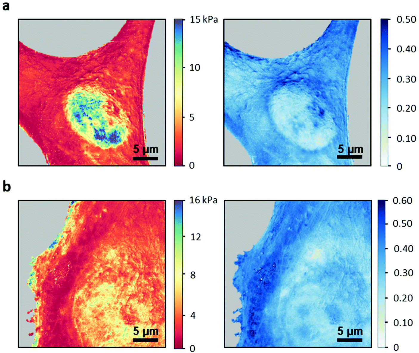 | ||
| Fig. 6 Nanomechanical maps of HeLa and NIH 3T3 cells. (a) HeLa. (b) NIH 3T3 cells. The fluidity exponent map reveals the presence of nucleoli inside the nucleous. FDCs taken at Fpeak = 3 nN, v = 150 μm s−1; maps of 512 × 512 pixels, FDC sample rate of 500 points per μm; z-displacement, 1.5 μm (HeLa), 2 μm (NIH 3T3). | ||
Conclusions
Experimental force–distance curves obtained on two different cell lines, HeLa and NIH 3T3, were compared to the analytical expressions deduced by applying linear elastic, linear viscoelastic and power-law rheology models. We showed that a cell experiencing a compressive force that involves indentations in the 1–2 μm range depended on the history of the deformation. This observation indicated the existence of energy dissipation processes within the cell. An elastic model provided two Young's modulus values for the same FDC. The lower value was obtained by fitting the approach section of the curve to the analytical expression. The larger value (Er ≈ 3Ea) was obtained by fitting the retraction section. There is not a straightforward criterion to select one value with respect to the other. For this reason, elastic models should not be used to provide quantitative characterization of the mechanical response of a live cell. This result is valid at least for experiments performed by applying relatively large deformations (say above 1 μm). Additional experiments need to be performed to generalize the above result to smaller indentations.The analytical force–distance curve generated using a 3D linear viscoelastic model presented a step discontinuity. This effect was associated with the use of triangular waveforms to generate the tip's displacement. It is associated with a discontinuity of the velocity at the turning point. On the other hand, the analytical force expression deduced for the 3D power-law model reproduced the experimental force–distance curves for HeLa and NIH 3T3 cell lines. These cell lines are very different in terms of mechanical properties and biological functionalities. Based on this result, we hypothesise that the same viscoelastic model might be applicable to other mammalian cells.
We showed that HeLa and fibroblast cells are harder to deform when the force is applied in a region of the plasma membrane located above the nucleus. A cell has higher compressive modulus values and lower fluidity exponents above the nucleus. The differences observed in the mechanical response of nuclear and cytoplasmic regions support the use of nanomechanical maps to characterize the spatial heterogeneity of a cell. The nanomechanical maps revealed structures that are hidden in the topographic images. Finally, we underlined the relevance of using analytical expressions that include bottom-effect corrections to compare experimental and theoretical force–distance curves.
Experimental methods
Cell culture and sample preparation
NIH3T3 fibroblasts (Sigma-Aldrich, UK) were cultured in Dulbecco's modified Eagle's medium-DMEM (Gibco Life Technologies, UK) supplemented with 10% fetal bovine serum-FBS (Gibco Life Technologies, UK), 1% penicillin/streptomycin FBS (Gibco Life Technologies, UK) and 2 mM L-glutamine (Sigma-Aldrich, Missouri, USA). They were maintained at 37 °C under a controlled atmosphere with 90% humidity and 5% of CO2. HeLa cells (Sigma-Aldrich, UK) were cultured in EMEM with 10% calf serum-CS (Gibco Life Technologies, UK), 1% penicillin/streptomycin (Gibco Life Technologies, UK) and 2 mM L-glutamine (Sigma-Aldrich, Missouri, USA). They were maintained at 37 °C under a controlled atmosphere with 90% humidity and 5% of CO2. The cells were seeded on an autoclaved glass cover slip for 24–48 h inside of a Petri Dish.To generate the nanomechanical maps of Fig. 6, NIH3T3 fibroblasts and HeLa cells were fixed with 4% formaldehyde (ThermoFisher Scientific, USA) in phosphate-buffered saline-PBS 0.01 M (Sigma-Aldrich, UK) for 10–15 minutes and rinsed with PBS.
Atomic force microscopy and FDCs
AFM measurements were performed using a JPK NanoWizard 3 AFM (JPK Instruments AG, Berlin, Germany) mounted on an Axio Observer D1 inverted microscope (Carl Zeiss, Oberkochen, Germany). The solid support was glass for the FDCs performed on live cells (Fig. 1–5) and a Petri dish for the nanomechanical maps (Fig. 6). The buffer used to record the FDCs was the culture medium. In Fig. 6, the imaging buffer was PBS. The temperature was kept constant at 37 °C using a temperature controller (BioCell™, JPK Instruments AG).We used BL-AC40TS cantilevers. Those cantilevers have pyramidal tips with an aperture semi angle of 18° (7 μm in height and a tip radius of 8 nm). The cantilever force constant k was calibrated using the thermal noise method.52,53 Force–distance curves on NIH 3T3 cells were recorded with k in the 0.10–0.13 N m−1 range (f0 = 38.15 kHz in liquid) while on HeLa cells the force constant was in the 0.044–0.087 N m−1 range (f0 = 30.68 kHz in liquid). The cantilever sensitivities were between 4.8–6.7 nm V−1 (NIH 3T3) and 6.9–9.5 nm V−1 (HeLa).
For each cell line, the data involved 8 single cells. For each cell, the FDCs were obtained on 12 different regions of the cell, 6 above the nucleus and 6 in cytoplasmatic region; 10 FDCs were obtained on each region of the cell.
The FDCs were obtained using a triangular waveform at 10 μm s−1. The indentation was stopped when the force reached a value of 3 nN. The z-displacement was performed with a closed-loop feedback and involved a z-displacement of 5 μm (sampling rate of 500 data points per μm). Hence the number of points was 2500 for the approach and 2500 for the retraction. The fittings were performed by applying a correlation coefficient R above 0.95.
The nanomechanical maps consisted of an ordered mesh of FDCs measured over the cell with a grid of 512 × 512 pixels. The velocity was 150 μm s−1 with a setpoint of 3 nN and a z-displacement of 1–1.5 μm. The sampling rate in the FDCs was 500 points per μm. The force constant and resonant frequency were, respectively, k = 0.13 N m−1 and f0 = 33.3 kHz (HeLa) and k = 0.16 N m−1f0 = 30.22 kHz (NIH 3T3).
Author contributions
J.G.S performed the simulations. F.M.E., R.M. and J.G.S. performed the experiments. R.G. conceived and supervised the project. R.G. wrote the manuscript. All the authors discussed the data and revised the manuscript.Conflicts of interest
There are no conflicts to declare.Acknowledgements
This project was supported by the Ministerio de Ciencia e Innovación (PID2019-106801GB-I00) and the Comunidad de Madrid S2018/NMT-4443 (Tec4Bio-CM).References
- J. Engler, S. Sen, H. L. Sweeney and D. E. Discher, Cell, 2006, 126, 677–689 CrossRef PubMed.
- A. Diz-Muñoz, O. D. Weiner and D. A. Fletcher, Nat. Phys., 2018, 14, 648–652 Search PubMed.
- T. Iskratsch, H. Wolfenson and M. P. Sheetz, Nat. Rev. Mol. Cell Biol., 2014, 15, 825–833 CrossRef CAS PubMed.
- P. Roca-Cusachs, V. Conte and X. Trepat, Nat. Cell Biol., 2017, 19, 742–751 CrossRef CAS PubMed.
- J. G. Goetz, S. Minguet, I. Navarro-Lérida, J. J. Lazcano, R. Samaniego, E. Calvo, M. Tello, T. Osteso-Ibáñez, T. Pellinen, A. Echarri, A. Cerezo, A. J. P. Klein–Szanto, R. Garcia, P. J. Keely, P. Sánchez-Mateos, E. Cukierman and M. A. Del Pozo, Cell, 2011, 146, 148–163 CrossRef CAS PubMed.
- Y. F. Dufrêne, T. Ando, R. Garcia, D. Alsteens, D. Martinez-Martin, A. Engel, C. Gerber and D. J. Müller, Nat. Nanotechnol., 2017, 12, 295–307 CrossRef PubMed.
- P.-H. Wu, D. R.-B. Aroush, A. Asnacios, W.-C. Chen, M. E. Dokukin, B. L. Doss, P. Durand-Smet, A. Ekpenyong, J. Guck, N. V. Guz, P. A. Janmey, J. S. H. Lee, N. M. Moore, A. Ott, Y.-C. Poh, R. Ros, M. Sander, I. Sokolov, J. R. Staunton, N. Wang, G. Whyte and D. Wirtz, Nat. Methods, 2018, 15, 491–498 CrossRef CAS PubMed.
- E. K. Dimitriadis, F. Horkay, J. Maresca, B. Kachar and R. S. Chadwick, Biophys. J., 2002, 82, 2798–2810 CrossRef CAS PubMed.
- H. Liu, J. Wen, Y. Xiao, J. Liu, S. Hopyan, M. Radisic, C. A. Simmons and Y. Sun, ACS Nano, 2014, 8, 3821–3828 CrossRef CAS PubMed.
- A. Rigato, A. Miyagi, S. Scheuring and F. Rico, Nat. Phys., 2017, 13, 771–775 Search PubMed.
- D. Martinez-Martin, G. Fläschner, B. Gaub, S. Martin, R. Newton, C. Beerli, J. Mercer, C. Gerber and D. J. Müller, Nature, 2017, 550, 500–505 CrossRef CAS PubMed.
- N. Mandriota, C. Friedsam, J. A. Jones-Molina, K. V. Tatem, D. E. Ingber and O. Sahin, Nat. Mater., 2019, 18, 1071–1077 CrossRef CAS PubMed.
- C. R. Guerrero, P. D. Garcia and R. Garcia, ACS Nano, 2019, 13, 9629–9637 CrossRef CAS PubMed.
- G. Zhou, B. Zhang, G. Tang, X.–F. Yu and M. Galluzzi, Adv. Phys. X, 2021, 6, 1866668 Search PubMed.
- M. Li, N. Xi, Y. Wang and L. Liu, Nano Res., 2019, 12, 703–718 CrossRef CAS.
- R. Garcia, Chem. Soc. Rev., 2020, 49, 5850–5884 RSC.
- I. N. Sneddon, Int. J. Eng. Sci., 1965, 3, 47–57 CrossRef.
- M. Lekka, K. Pogoda, J. Gostek, O. Klymenko, S. Prauzner-Bechcicki, J. Wiltowska-Zuber, J. Jaczewska, J. Lekki and Z. Stachura, Micron, 2012, 43, 1259–1266 CrossRef PubMed.
- J. R. Ramos, J. Pabijan, R. Garcia and M. Lekka, Beilstein J. Nanotechnol., 2014, 5, 447–457 CrossRef PubMed.
- J. R. Staunton, B. L. Doss, S. Lindsay and R. Ros, Sci. Rep., 2016, 6, 19686 CrossRef CAS PubMed.
- C. Alibert, B. Goud and J.-B. Manneville, Biol. Cell, 2017, 109, 167–189 CrossRef PubMed.
- A. Calzado-Martín, M. Encinar, J. Tamayo, M. Calleja and A. San Paulo, ACS Nano, 2016, 10, 3365–3374 CrossRef PubMed.
- C. Rotsch and M. Radmacher, Biophys. J., 2000, 78, 520–535 CrossRef CAS PubMed.
- H. W. Wu, T. Kuhn and V. T. Moy, Scanning, 1998, 20, 389–397 CrossRef CAS PubMed.
- P. D. Garcia, C. R. Guerrero and R. Garcia, Nanoscale, 2017, 9, 12051–12059 RSC.
- H. Schillers, C. Rianna, J. Schäpe, T. Luque, H. Doschke, M. Wälte, J. J. Uriarte, N. Campillo, G. P. A. Michanetzis, J. Bobrowska, A. Dumitru, E. T. Herruzo, S. Bovio, P. Parot, M. Galluzzi, A. Podestà, L. Puricelli, S. Scheuring, Y. Missirlis, R. Garcia, M. Odorico, J.-M. Teulon, F. Lafont, M. Lekka, F. Rico, A. Rigato, J.-L. Pellequer, H. Oberleithner, D. Navajas and M. Radmacher, Sci. Rep., 2017, 7, 5117 CrossRef PubMed.
- P. Kollmannsberger and B. Fabry, Annu. Rev. Mater. Res., 2011, 41, 75–97 CrossRef CAS.
- P. Kollmannsberger, C. T. Mierke and B. Fabry, Soft Matter, 2011, 7, 3127–3132 RSC.
- S. Moreno-Flores, R. Benitez, M. Vivanco and J. L. Toca-Herrera, Nanotechnology, 2010, 21, 445101 CrossRef PubMed.
- A. X. Cartagena-Rivera, W. H. Wang, R. L. Geahlen and A. Raman, Sci. Rep., 2015, 5, 11692 CrossRef CAS PubMed.
- B. R. Bruckner, H. Nöding and A. Janshoff, Biophys. J., 2017, 112, 724–735 CrossRef PubMed.
- P. D. Garcia, C. R. Guerrero and R. Garcia, Nanoscale, 2020, 12, 9133–9143 RSC.
- P. D. Garcia and R. Garcia, Biophys. J., 2018, 114, 2923–2932 CrossRef CAS PubMed.
- P. D. Garcia and R. Garcia, Nanoscale, 2018, 10, 19799–19809 RSC.
- F. M. Hecht, J. Rheinlaender, N. Schierbaum, W. H. Goldmann, B. Fabry and T. E. Schäffer, Soft Matter, 2015, 11, 4584–4591 RSC.
- J. S. de Sousa, J. A. C. Santos, E. B. Barros, L. M. R. Alencar, W. T. Cruz, M. V. Ramos and J. Mendes-Filho, J. Appl. Phys., 2017, 121, 034901 CrossRef.
- J. S. de Sousa, R. S. Freire, F. D. Sousa, M. Radmacher, A. F. B. Silva, M. V. Ramos, A. C. O. Monteiro-Moreira, F. P. Mesquita, M. E. A. Moraes, R. C. Montenegro and C. L. N. Oliveira, Sci. Rep., 2020, 10, 4749 CrossRef CAS PubMed.
- Y. M. Efremov, T. Okajima and A. Raman, Soft Matter, 2019, 16, 64–81 RSC.
- Y. M. Efremov, W.-H. Wang, S. D. Hardy, R. L. Geahlen and A. Raman, Sci. Rep., 2017, 7, 1541 CrossRef PubMed.
- N. Schierbaum, J. Rheinlaender and T. E. Schäffer, Soft Matter, 2019, 15, 1721–1729 RSC.
- H. Hubrich, I. P. Mey, B. R. Brückner, P. Mühlenbrock, S. Nehls, L. Grabenhorst, T. Oswald, C. Steinem and A. Janshoff, Nano Lett., 2020, 20, 6329–6335 CrossRef CAS PubMed.
- Y. M. Efremov, S. L. Kotova and P. S. Timashev, Sci. Rep., 2020, 10, 13302 CrossRef CAS PubMed.
- A. Cordes, H. Witt, A. Gallemí-Pérez, B. Brückner, F. Grimm, M. Vache, T. Oswald, J. Bodenschatz, D. Flormann, F. Lautenschläger, M. Tarantola and A. Janshoff, Phys. Rev. Lett., 2020, 125, 068101 CrossRef CAS PubMed.
- A. Bonfanti, J. L. Kaplan, G. Charras and A. Kabla, Soft Matter, 2020, 16, 6002–6020 RSC.
- T. C. T. Ting, J. Appl. Mech., 1966, 33, 845–854 CrossRef.
- C. J. Gomez and R. Garcia, Ultramicroscopy, 2010, 110, 626–633 CrossRef CAS PubMed.
- N. Guz, M. Dokukin, V. Kalaparthi and I. Sokolov, Biophys. J., 2014, 107, 564–575 CrossRef CAS PubMed.
- S. Santos, K. Gadelrab, C.-Y. Lai, T. Olukan, J. Font, V. Barcons, A. Verdaguer and M. Chiesa, J. Appl. Phys., 2021, 129, 134302 CrossRef CAS.
- C. H. Parvini, M. A. S. R. Saadi and S. D. Solares, Beilstein J. Nanotechnol., 2020, 11, 922–937 CrossRef CAS PubMed.
- G. Tang, M. Galluzzi, B. Zhang, Y.-L. Shen and F. J. Stadler, Langmuir, 2019, 35, 7578–7587 CrossRef CAS PubMed.
- E. Moeendarbary, L. Valon, M. Fritzsche, A. R. Harris, D. A. Moulding, A. J. Thrasher, E. Stride, L. Mahadevan and G. T. Charras, Nat. Mater., 2013, 12, 253–261 CrossRef CAS PubMed.
- Y. M. Efremov, S. L. Kotova, A. A. Akovantseva and P. S. Timashev, J. Nanobiotechnol., 2020, 18, 134 CrossRef CAS PubMed.
- J. L. Hutter and J. Bechhoefer, Rev. Sci. Instrum., 1993, 64, 1868 CrossRef CAS.
- R. Garcia, Amplitude Modulation AFM, Wiley-VCH, Weinheim, Germany, 2010 Search PubMed.
| This journal is © The Royal Society of Chemistry 2021 |