
 Open Access Article
 This Open Access Article is licensed under a Creative Commons Attribution-Non Commercial 3.0 Unported Licence
Unlocking the decoding of unknown magnetic nanobarcode signatures†
Mohammad Reza
Zamani Kouhpanji
 ab and
Bethanie J. H.
Stadler
*ac
ab and
Bethanie J. H.
Stadler
*ac
aDepartment of Electrical and Computer Engineering, University of Minnesota Twin Cities, Minneapolis, MN 55455, USA
bDepartment of Biomedical Engineering, University of Minnesota Twin Cities, Minneapolis, MN 55455, USA
cDepartment of Chemical Engineering and Materials Science, University of Minnesota Twin Cities, Minneapolis, MN 55455, USA. E-mail: stadler@umn.edu; Tel: +1 612 626 1628
First published on 9th December 2020
Abstract
Magnetic nanowires (MNWs) rank among the most promising multifunctional magnetic nanomaterials for nanobarcoding applications owing to their safety, nontoxicity, and remote decoding using a single magnetic excitation source. Until recently, coercivity and saturation magnetization have been proposed as encoding parameters. Herein, backward remanence magnetization (BRM) is used to decode unknown remanence spectra of MNWs-based nanobarcodes. A simple and fast expectation algorithm is proposed to decode the unknown remanence spectra with a success rate of 86% even though the MNWs have similar coercivities, which cannot be accomplished by other decoding schemes. Our experimental approach and analytical analysis open a promising direction towards reliably decoding magnetic nanobarcodes to expand their capabilities for security and labeling applications.
1. Introduction
Nanobarcodes are an inseparable part of daily lives, playing a critical role in industry heavyweights, such as the car industry, the food industry, and the medical industry. Encoding and decoding techniques are the two main bottlenecks hindering the successful interchange of nanobarcodes within diverse applications.1 As a result, numerous types of nanobarcodes, such as photonic nanoparticles,2–4 magnetic nanoparticles,5–7 and magneto-optic nanoparticles,8 have emerged to meet the desired requirements for individual applications. The synthesis approach of nanobarcodes can allow one to engineer multiple properties, such as absorption/emission spectra of photonic nanoparticles,9–11 coercivity and saturation magnetization of magnetic nanoparticles,7,12–15 to leverage their encoding through various synthesis strategies, both chemical and physical strategies.16–19 However, producing nanobarcodes with diverse encodings does not necessarily guarantee their successful decoding. For example, it was shown the magnetic signature of magnetic nanowires (MNWs) could be engineered by tuning their dimensions and compositions to provide several magnetic nanobarcodes.19 Even though these magnetic nanobarcodes render unique magnetic signatures while being measured individually, decoding their magnetic signature from the measurements of unknown combinations has not been demonstrated. This problem is not limited to magnetic nanobarcodes because other nanobarcodes, such as optical, radio-frequency identification (RFID), and morphological-based nanobarcodes, also suffer from this problem.1We believe this technological limitation, inability to decode unknown combinations of magnetic nanobarcodes, is due to the magnetic measurements and a lack of a robust analytical approaches for decoding the measured magnetic signature. For example, the hysteresis loop method has been widely used to measure the saturation magnetization (Ms) and coercivity (Hc) as magnetic signatures for decoding the magnetic nanobarcodes.7,12,14,20,21 Since the hysteresis loop method only provides averaged values for Ms and Hc, it does not provide any insight for decoding them if there is no prior knowledge about the number and types of magnetic nanobarcodes at the readout. More importantly, even though other magnetic measurements, such as first-order reversal curves (FORC)22–25 and magnetic nanoparticles spectroscopy,26–28 provide distributions as magnetic signatures, there is still a lack of robust analytical approaches to reliably decode the measured magnetic signatures without prior knowledge about the magnetic nanobarcodes.
To overcome these limitations, we propose to use magnetic remanence measurements as they can provide three main advantages compared to the aforementioned methods. First, the magnetic remanence measurements provide a unique remanence spectrum for the magnetic nanobarcodes that is related to the Hc, the Hc standard deviation, interaction fields (Hu), and their correlations, in contrast to the hysteresis loop measurements only provide a single value for decoding. Second, similar to the FORC method, the remanence measurement provides remanence distributions instead of single values, and it is significantly faster than FORC measurement. Lastly yet most importantly, the remanence measurements measure the magnetization at zero applied field, so there is no background signal to reduce its sensitivity. Indeed, the standard remanence measurements, isothermal remanence magnetization (IRM) and DC demagnetization (DCD) measurements, have been widely used in rock magnetism for predicting the unknown magnetic phases in natural minerals.29–34 According to the Stoner–Wohlfarth model, the IRM and DCD spectra are identical for non-interacting MNWs (Hu = 0), but they will yield different results when Hu is not negligible. Since Hu dictates the initial and final magnetization states, the initial magnetization state of an array of MNWs plays an important role in their magnetic remanence. Therefore, to further enhance the reliability and reproducibility decoding using the remanence spectra, we propose to use a modified remanence measurement that is different from the standard remanence measurements. We reported our protocol for this method, named “backward remanence magnetization (BRM)”, in our previous work.35 Details about the BRM measurement and how it is beneficial compared to the IRM and DCD measurements are fully discussed in ESI† using experimental comparison. An expectation algorithm was used to decode unknown magnetic remanence spectra that will be fully described in the experimental and analytical section below.
More specifically, in this study, we measure the magnetic remanence spectra of several MNWs arrays inside polycarbonate templates using the BRM measurement to investigate the capability of the BRM method and the expectation algorithm for decoding unknown combinations of MNWs arrays. The BRM spectra of magnetic nanobarcodes were engineered by composition and geometrical parameters, e.g. diameter and interwire distance—characterized by the filling factor of the polycarbonate templates. Next, we prepared several combinations of magnetic nanobarcodes and re-measured their magnetic remanence spectra. We show that the ∼86% of all ‘unknown’ combinations of two magnetic nanobarcodes can be reliably decoded using our algorithm. We also discuss the fundamentals of our experimental and analytical approaches to improve the decoding rate when there are more than two magnetic nanobarcodes in unknown combinations.
2. Experimental and analytical approaches
As proof of concept, several MNWs were electrodeposited in polycarbonate templates, Fig. 1.36–38 Details about the three-electrode electrodeposition technique are given in the ESI.† Specifically, we tailored the magnetic remanence spectra of the eight magnetic nanobarcodes that can be classified into two groups according to their compositions, diameters, and filling factors (defined as the ratio of the MNWs to the templates). The first group was made of nickel (Ni) and another was made of iron:cobalt (Fe65Co35) alloy. Each group included four MNWs types with the same interwire distance but different diameters. Therefore, the filling factor was adjusted using the MNWs diameter. The diameter (filling factor) are 30 nm (∼0.5%), 50 nm (∼1%), 100 nm (∼2%), and 200 nm (∼12%). Note the filling factor helps to tune the interaction fields (Hu) among the MNWs inside the templates. To reach the highest saturation remanence (Msr), it is necessary to assure that the shape anisotropy and crystal anisotropy are in the same direction to induce uniaxial anisotropy along the MNWs long axis (here, we tailored the MNWs to have their long axis as their easy axis). We fabricated the MNWs with aspect ratios (length to diameter) >10, see SEM images given in ESI,† to have the shape anisotropy along the MNWs easy axis leading to a magnetically bi-stable condition. Furthermore, we adjusted the electrodeposition parameters, such as bath composition, pH, and deposition voltage, to have crystal anisotropy along the MNWs easy axis, see the XRD results given in ESI.† We chose Ni and FeCo because they have almost the same crystal anisotropy, therefore, we can have the same coercivity (Hc) but they have very different saturation magnetizations (Ms = 0.63 and 2.45 T, respectively). Furthermore, since Ni and FeCo have significantly different magnetic moments, we chose them to tune Hu for the same diameter and filling factor.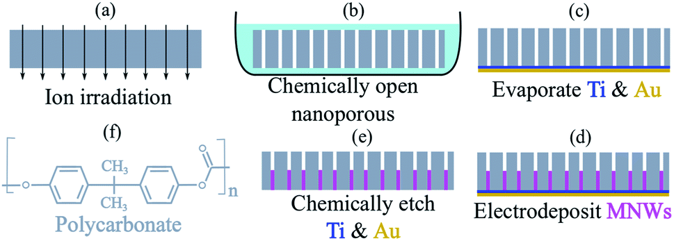 | ||
| Fig. 1 A schematic depicting magnetic nanobarcodes synthesis procedure, dimensions are not drawn to scale. (a) The ion irradiation of a raw polycarbonate foil (grey), (b) chemical etching (light blue) of the ion irradiated polycarbonate, (c) evaporation of Ti (blue) then Au (yellow) for a back contacts, (d) electrodeposition of MNWs (pink), and (e) a combination wet and dry etch process to remove the back contacts. (f) The chemical structure of polycarbonate. Further details are in ESI.† | ||
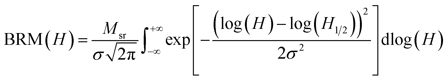
To realize the strength of remanence spectra for encoding, we systematically measured the remanence spectra using the backward remanence magnetization (BRM) technique, see ESI† for more details. Briefly, samples are saturated using a positive field before applying and removing a negative field. The positive saturation is repeated before applying and removing progressively more negative fields. Each time the negative field is removed (H = 0), the remanent moment is measured and normalized by the sample's remanent saturation magnetization (Msr), as shown in Fig. 2. Msr is the amplitude of each BRM spectrum, and it is equal to the hysteresis loop remanence, or the amount of the magnetic material in each magnetic nanobarcode that is magnetically stable once the field (H) is removed after saturation.
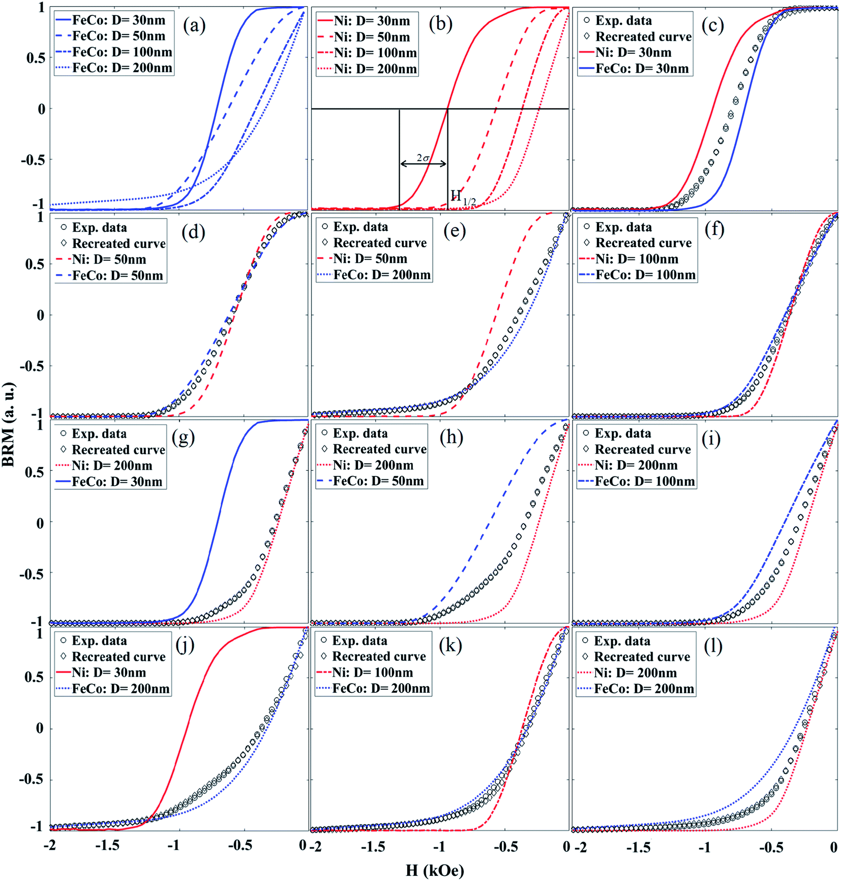 | ||
| Fig. 2 The backward remanence magnetization (BRM) spectra of the individual MNWs arrays: (a) FeCo and (b) Ni of various diameters as marked. (c–l) BRM spectra for several combinations (according to the legends). The individual BRM spectra were linearly summed (recreated curves) and compared with the measured BRM of the combinations (exp. data). (b) Shows H1/2 (the field at the center of the BRM spectrum, where BRM = 0) and σ (the dispersion parameter), which are used to describe the BRM spectra below. | ||
To utilize the BRM spectra for decoding, we combined at least two different types of magnetic nanobarcodes and measured the BRM spectra of each combination, labeled as “Exp. data” in Fig. 2. Then the BRM spectra of these combinations were compared with the linear summation of the weighted BRM spectra of the known individual magnetic nanobarcodes in the combination, labeled as “Recreated curve” in Fig. 2. As can be seen in Fig. 2, a very good agreement between the “Exp. data” and the “Recreated curve” was achieved. The weights were also used to calculate the volume ratio of each magnetic nanobarcode; the details and results are given in ESI.† The good agreement between the “Exp. data” and the “Recreated curve” indicates that the MNWs from one nanobarcode do not cross-talk with the MNWs of the other nanobarcodes in the combination. Therefore, the BRM spectra can be linearly summed for decoding. For practical applications, where two different subjects are labeled using magnetic nanobarcodes, the physical distance between the magnetic nanobarcodes will be significantly larger than the interwire distances used here (∼500 nm), see SEM images in ESI.† This observation is our hypothesis for using a cumulative log-normal distribution, which was proposed by ref. 39 and 40 for unmixing unknown mixtures of natural minerals with complex geometries in rock magnetism. This cumulative log-normal distribution is
 | (1) |
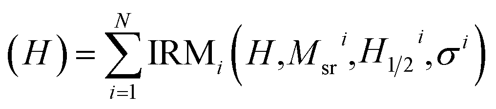 | (2) |
For an unknown BRM spectrum, in addition to Msri, H1/2i, and σi; the number of magnetic nanobarcodes (N) is also unknown. Undoubtedly, increasing the N improves the fitting quality (defined as the root mean square (RMS) error between eqn (2) and the experimentally measured BRM spectra) leading to boundless values for N. However, after a certain increase in N, the RMS error does not improve, and it converges to a constant value. Therefore, to determine number of the magnetic nanobarcodes in an unknown combination, we use the expectation algorithm similar to what was proposed and developed by ref. 42–44. Briefly, we assume there are N types of unknown magnetic nanobarcodes in an unknown combination. We fit eqn (2) to the BRM spectra of the unknown combination to calculate the BRM parameters for each N types of magnetic nanobarcodes. Then, we construct the BRM spectra of the combination using eqn (1) and (2) and we calculate the RMS error between the constructed BRM spectra and the experimental BRM spectra. Next, we increase the number of nanobarcodes to N + 1 and repeat the fitting to find the new set of the remanence parameters and recalculate the RMS error of the new fit. At this point, the new RMS error is compared with the previous RMS error to evaluate how much the RMS error is improved. If the RMS improvement is not significant, we stop the procedure and the number of magnetic nanobarcodes is equal to the N of the previous step. However, if the RMS error improvement is significant, we increase the number of magnetic nanobarcodes to N + 2 and repeat the procedure. The “significant” improvement of the RMS error depends on the number of nanobarcodes and how unique their BRM spectra are. For example, we found a 50% hierarchy improvement is sufficient to correctly decode unknown combinations, as discussed below. Eventually, these N BRM spectra were individually compared with the BRM spectrum of each individual magnetic nanobarcode to find the best matches, as discussed below and tabulated in Table 1.
| Best matches | Ni30:FeCo30 | Ni30:FeCo50 | Ni30:FeCo100 | Ni30:FeCo200 | ||||
| RMS for best matches (%) | 6 | 22 | 6 | 24 | 15 | 10 | 4 | 4 |
| Best matches | Ni50:FeCo30 | Ni50:FeCo50 | Ni50:FeCo100 | Ni50:FeCo200 | ||||
| RMS for best matches (%) | 10 | 25 | 12 | 17 | 6 | 24 | 15 | 11 |
| Best matches | Ni100:FeCo30 | Ni100:FeCo50 | Ni100:FeCo100 | Ni100:FeCo200 | ||||
| RMS for best matches (%) | 14 | 26 | 10 | 12 | 10 | 11 | ||
| Best matches | Ni200:FeCo30 | Ni200:FeCo50 | Ni200:FeCo100 | Ni200:FeCo200 | ||||
| RMS for best matches (%) | 5 | 7 | 12 | 13 | 10 | 13 | ||
| Best matches | Ni30:Ni50 | Ni50:Ni100 | FeCo30:FeCo50 | FeCo50:FeCo100 | ||||
| RMS for best matches (%) | 8 | 17 | 15 | 16 | 7 | 15 | ||
| Best matches | Ni30:Ni100 | Ni50:Ni200 | FeCo30:FeCo100 | FeCo50:FeCo100 | ||||
| RMS for best matches (%) | 3 | 4 | 20 | 23 | 7 | 18 | ||
| Best matches | Ni30:Ni200 | Ni100:Ni200 | FeCo30:FeCo200 | FeCo100:FeCo200 | ||||
| RMS for best matches (%) | 3 | 3 | 9 | 18 | 6 | 9 | 10 | 27 |
3. Results
Before walking through the decoding procedure, we first explain the BRM spectra features and how the MNWs dimensions and compositions can tailor them. As mentioned above Msr shows the amount of the magnetic material in each magnetic nanobarcode that is magnetically stable once the field (H) is removed after saturation. In contrast, the curvature of the BRM spectra determines the intrinsic response of the magnetic nanobarcodes related to its coercivity (Hc), Hc standard deviation, interaction field (Hu), and their correlations. The curvature of the BRM spectra can be indexed by the field where BRM is zero (H1/2) and its broadening (2σ) that shows how fast it responds to variations of H, these parameters are labeled in Fig. 2b. Note, if one takes a derivative of BRM spectra (dBRM), the dBRM will be similar to a Gaussian distribution, in which its maximum is located at H1/2 and its standard deviation is σ; the dBRM spectra are given in the ESI.†H 1/2 and σ are correlated to the magnetic moment (Ms), Hc, relative strength of Hc and Hu, and the standard deviation of Hc, which is related to MNWs compositions and the pore size distributions of the templates. Since the BRM spectra are measured at zero applied field, the total field experienced by each MNW inside the nanobarcode is simply the Hu among the MNWs. If the Hu is larger than the MNWs Hc, it causes some MNWs to switch until an equilibrium state is reached, where the magnetization at the equilibrium state is called the remanence, or remenant magnetization. Since Hu is maximum after saturation of MNWs, analyzing the squareness (Msr/Ms) is the simplest way to understand the relative strength of the Hu and Hc for the MNWs in this study. Thus, the Hc, H1/2, σ, and squareness of our magnetic nanobarcodes are given in Fig. 3. Hc is a function of the shape anisotropy and crystal anisotropy. Both Ni and FeCo MNWs have the same Hc and it reduces as the MNWs diameter increases, Fig. 3a. Since the Ni and FeCo MNWs have similar dimensions, it can be concluded that the shape anisotropy is the dominant term determining the Hc. Note H1/2 is dominantly determined by Hc, so they are the same for our MNWs, see Fig. 3a. Furthermore, since FeCo has higher magnetic moment (∼2.45 T) compared to Ni (∼0.63 T), the FeCo MNWs have larger Hu compared to the Ni MNWs for the same diameter and filling factor. Therefore, the FeCo MNWs have smaller squareness compared to the Ni MNWs, see Fig. 3b, and the squareness decreases as the diameter increases due to the fact that the Hc decreases. Even though the Hc decreases as the diameter increases, σ is fairly constant. Since all templates were prepared in the same way, this indicates that the pore size distributions were the same for all of our magnetic nanobarcodes and it profoundly impacts σ compared to Hu. Indeed, because the FeCo magnetic nanobarcodes had higher Hu (due to larger Ms), they have larger σ which shows that Hu only causes a vertical shift in σ. Note, the MNWs with 30 nm diameter are non-interacting, Hu ≈ 0, thus they have similar σ values. Therefore, it can be realized that the curvature of the BRM spectra, see Fig. 2, can be tailored using the MNWs composition and diameter to achieve unique BRM spectra, which we will explain how to decode in the discussion section.
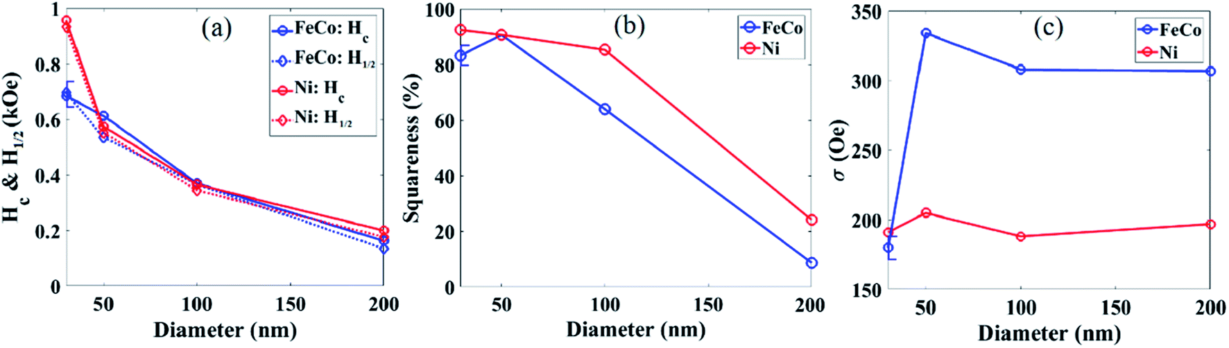 | ||
| Fig. 3 Magnetic parameters that were tailored to produce unique BRM spectra, (a) coercivity (Hc) and half BRM field (H1/2), (b) squareness (Msr/Ms), and (c) the broadening parameter (σ). See ESI† for hysteresis loops (Hc, Msr, Ms) and Fig. 2b for BRM spectra (H1/2, σ). The maximum error bar (n = 2) for subfigures (a–c) are shown. | ||
4. Discussion
To demonstrate our analytical approach for the decoding of unknown BRM spectra, here we prepared unknown combinations of magnetic nanobarcodes and measured their BRM spectra. For simplicity, we prepared unknown combinations of two magnetic nanobarcodes, and this can be increased to larger numbers of magnetic nanobarcodes in the same fashion. To decode any unknown BRM spectra, the first and most important step is to determine the number of magnetic nanobarcodes composing the unknown BRM spectra. As illustrated in the result section, the magnetic nanobarcodes were engineered using the MNW compositions and diameters to have distinct BRM spectra, which can be indexed by the Msr, H1/2, and σ parameters. Once the number of the magnetic nanobarcodes is determined correctly, identifying the present type of the magnetic nanobarcode can be readily accomplished by comparing the fitting results (Msr, H1/2, and σ) with those of the magnetic nanobarcodes to find the best match.Fig. 4 shows the results for determining the number (N) of magnetic nanobarcodes in unknown combinations of magnetic nanobarcodes. The important feature in these curves is the N at which the RMS error reaches a plateau, which is why the curves were normalized with respect to the RMS error found by matching the experimental data to N = 1. According to our procedure in the experimental and analytical approaches section above, we first assume the unknown sample is made up of only one magnetic nanobarcode (N = 1). Therefore, we fit its BRM spectrum to a single BRM(H) function given in eqn (1) and calculate the RMS error. For example, the curve labeled by a star in Fig. 4b was fit to one BRM curve with Msr, H1/2 and σ proportional to 7.8, 6.2, and 0.9 of the actual values, respectively, but the RMS1 error (the superscript “1” indicates N = 1) for was 22%. Also, these values do not match any of the samples in Fig. 3.
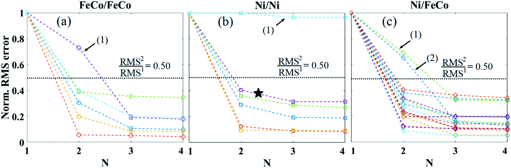 | ||
| Fig. 4 RMS error as a function of the assumed number of magnetic nanobarcodes (N) in unknown combinations, normalized to the RMS error of the best fit to N = 1. As the N increases, the RMS error decreases for combination samples until N equals the real number of the magnetic nanobarcodes in each unknown combination. Here all unknown combinations were prepared with two magnetic nanobarcodes. The combinations shown each had varying diameters with (a) both FeCo, (b) both Ni, and (c) one Ni and one FeCo magnetic nanobarcodes. The unsuccessful decodings were shown by arrows. | ||
Next, we assume there were two magnetic nanobarcodes (N = 2) forming the unknown BRM spectrum. In this case, two BRM(H) function were linearly added according to eqn (2) and the resulting function was fitted to the unknown BRM spectrum. In this case, the RMS2 error (the superscript “2” indicates N = 2) was found to be 9% for the same labeled curve in Fig. 4b. By comparing RMS1 and RMS2, the RMS2 error was decreased by a factor of 2.4 (∼40% of the RMS1 error). Next, we increased the number of magnetic nanobarcodes to three (N = 3) and recalculated the RMS3 error, which was 7%, or 22% of RMS2, see N = 3 point for the starred curve in Fig. 4b. RMS4 error for this same sample was calculated as 7% again, which means zero improvement in the RMS, so we stopped the decoding procedure.
To determine the number of magnetic nanobarcodes in this unknown combination, it is critical to answer “what reduction percentage is optimum?” For unknown combinations of our magnetic nanobarcodes, we found a 50% reduction of the RMS error in each step (RMSi+1 ≤ 50% of RMSi, superscript “i” indicates ith step of decoding) is sufficient to determine the number of magnetic nanobarcodes in unknown BRM spectra. Choosing 50% reduction, we managed to successfully decode 24 out of 28 (∼86% success rate) unknown combinations of two magnetic nanobarcodes. If the chosen reduction percentage is too small, the determined number of magnetic nanobarcodes will be incorrectly large. In contrast, choosing a large reduction percentage can cause the determined number of the magnetic nanobarcodes to be incorrectly small. This latter case is observed in Fig. 4 (arrows) where all of the samples contained only 2 barcodes (N = 2). Moreover, we can improve the decoding rate further in at least two ways. First, we can design and synthesize multi-segmented or multi-component MNWs to engineer the magnetic anisotropy for minimal overlap in nanobarcode signatures.45–48 Second, more advanced decoding algorithms based on machine learning can be implemented.
Once the number of the magnetic nanobarcodes in an unknown combination is determined, we compare the fitting results (Msr, H1/2, and σ) to those of our magnetic nanobarcodes to find the best match indicating the type of magnetic nanobarcodes in the unknown combination. The best match was found by calculating the lowest RMS error between the BRM spectra of the individual magnetic nanobarcodes and the fitting results. Table 1 shows the best matches and the corresponding RMS errors.
As mentioned in experimental and analytical section, we intentionally chose the Ni and FeCo because they have roughly the same crystal anisotropy, so Hc is only a function of the MNWs diameter except for the smallest diameter (30 nm), see Fig. 3a. In the 30 nm diameter case, the mechanism of reversal most likely changes for the low moment Ni nanowires to coherent rotation vs. vortex walls, which are likely the mechanism in all other cases based on simulations.48 Furthermore, the templates for electrodeposition of the MNWs were prepared in the same way thus the σ is only a function of composition, Ni or FeCo, and not diameter except for the 30 nm sample, see Fig. 3c. The 30 m samples have the lowest interactions between nanowires (lowest filling factor templates), which is likely why σ of FeCo matches Ni in this case.
Therefore, it can be realized that indeed there was only one encoding parameter when decoding the magnetic nanobarcodes with the same composition or the same diameter. These results indicate the unprecedented advantage of the BRM measurement compared to the current state of the art, such as the hysteresis loop measurement or magnetic nanoparticle spectroscopy.1 Specifically, hysteresis loops only provide a single value for Hc and Ms that cannot be used to distinguish between the different types of magnetic nanobarcodes in an unknown combinations. Moreover, since the BRM measurement is able to decode the magnetic nanobarcodes with only one distinct encoding, it can boost the number of codes.
5. Conclusion
In this study, we explore the application of the backward remanence magnetization (BRM) measurement for decoding unknown combinations of magnetic nanobarcodes prepared by electrodeposition of magnetic nanowires (MNWs) inside polycarbonate templates. Using an expectation algorithm, we decoded unknown combinations of the magnetic nanobarcodes by determining the number and types of the present magnetic nanobarcode in the unknown combinations. We indexed the BRM spectra of the magnetic nanobarcodes using two parameters (1) the field where the BRM spectra is zero (H1/2) and (2) its broadening (σ) that demonstrates how fast the BRM spectra raise from zero to its maximum. We illustrated the dependency of these two parameters to the magnetic moment (Ms), coercivity (Hc), standard deviation of Hc, interaction field (Hu), and the correlation of Hc and Hu, which we engineered using the MNWs diameter and composition. Our experimental observations show that the BRM measurement is a promising approach to decode unknown combinations as far as only one of these two parameters (H1/2 and σ) is unique. This indicates that our experimental and analytical approach is able to decode even a combination of magnetic nanobarcodes with similar Hc, something that is impossible to be done using the most commonly techniques for decoding, such as hysteresis loop method. More importantly, enabling the decoding of magnetic nanobarcodes with only one unique parameters paves the route to readily expand the number of magnetic nanobarcodes. Furthermore, this expectation algorithm can be used with other methods, such as magnetic nanoparticle spectroscopy, for decoding magnetic nanobarcodes.Data availability
All presented data in this manuscript will be provided by the corresponding author under a reasonable request.Conflicts of interest
There are no conflicts to declare.Acknowledgements
This work is primarily supported by the National Science Foundation (NSF) under grant number CMMI-1762884. Part of this work was performed at the Institute for Rock Magnetism (IRM) at the University of Minnesota. The IRM is a US National Multi-user Facility supported through the Instrumentation and Facilities program of the National Science Foundation, Earth Sciences Division (NSF/EAR 1642268), and by funding from the University of Minnesota. Portions of this work were conducted in the Minnesota Nano Center, which is supported by the National Science Foundation through the National Nano Coordinated Infrastructure Network (NNCI) under Award Number ECCS-2025124. Parts of this work were also carried out in the Characterization Facility, University of Minnesota, which receives partial support from NSF through the MRSEC program.References
- S. Shikha, T. Salafi, J. Cheng and Y. Zhang, Versatile design and synthesis of nano-barcodes, Chem. Soc. Rev., 2017, 46, 7054–7093, 10.1039/c7cs00271h.
- A. G. Mark, J. G. Gibbs, T. C. Lee and P. Fischer, Hybrid nanocolloids with programmed three-dimensional shape and material composition, Nat. Mater., 2013, 12, 802–807, DOI:10.1038/nmat3685.
- S. Kalytchuk, Y. Wang, K. Poláková and R. Zbořil, Carbon Dot Fluorescence-Lifetime-Encoded Anti-Counterfeiting, ACS Appl. Mater. Interfaces, 2018, 10, 29902–29908, DOI:10.1021/acsami.8b11663.
- A. Hlaváček, J. Křivánková, J. Přikryl and F. Foret, Photon-Upconversion Barcoding with Multiple Barcode Channels: Application for Droplet Microfluidics, Anal. Chem., 2019, 91(20), 12630–12635 CrossRef PubMed.
- L. Clime, S. Y. Zhao, P. Chen, F. Normandin, H. Roberge and T. Veres, The interaction field in arrays of ferromagnetic barcode nanowires, Nanotechnology, 2007, 18(43), 435709 CrossRef.
- S. Moraes, D. Navas, F. Béron, M. Proenca, K. Pirota, C. Sousa and J. Araújo, The Role of Cu Length on the Magnetic Behaviour of Fe/Cu Multi-Segmented Nanowires, Nanomaterials, 2018, 8, 490, DOI:10.3390/nano8070490.
- Y. S. Jeon, H. M. Shin, Y. J. Kim, D. Y. Nam, B. C. Park, E. Yoo, H.-R. Kim and Y. K. Kim, Metallic Fe–Au Barcode Nanowires as a Simultaneous T Cell Capturing and Cytokine Sensing Platform for Immunoassay at the Single-Cell Level, ACS Appl. Mater. Interfaces, 2019, 11, 23901–23908, DOI:10.1021/acsami.9b06535.
- D. S. Koktysh and W. Pham, A combinatorial approach for the fabrication of magneto-optical hybrid nanoparticles, Int. J. Nanomed., 2019, 14, 9855–9863, DOI:10.2147/ijn.S228962.
- X. Zhao, W. Zhang, X. Qiu, Q. Mei, Y. Luo and W. Fu, Rapid and sensitive exosome detection with CRISPR/Cas12a, Anal. Bioanal. Chem., 2020, 412, 601–609, DOI:10.1007/s00216-019-02211-4.
- J. Zhu, P. Zhao, J. Yang, J. Shi, J. Chu, W. Miao, Y. Zhao and B. Zhou, Sharpening upconversion nanoparticles to reduce surface quenching, Dalton Trans., 2020, 49, 285–288, 10.1039/c9dt04266k.
- H. Li, M. Tan, X. Wang, F. Li, Y. Zhang, L. Zhao, C. Yang and G. Chen, Temporal multiplexed in vivo upconversion imaging, J. Am. Chem. Soc., 2020, 142(4), 2023–2030 CrossRef CAS PubMed.
- S. J. Yoon, B. G. Kim, I. T. Jeon, J. H. Wu and Y. K. Kim, Compositional Dependence of Magnetic Properties in CoFe/Au Nanobarcodes, Appl. Phys. Express, 2012, 5, 103003, DOI:10.1143/apex.5.103003.
- I. T. Jeon, S. J. Yoon, B. G. Kim, J. S. Lee, B. H. An, J.-S. Ju, J. H. Wu and Y. K. Kim, Magnetic NiFe/Au barcode nanowires with self-powered motion, J. Appl. Phys., 2012, 111, 07B513, DOI:10.1063/1.3676062.
- J. H. Lee, J. H. Wu, H. L. Liu, J. U. Cho, M. K. Cho, B. H. An, J. H. Min, S. J. Noh and Y. K. Kim, Iron-gold barcode nanowires, Angew. Chem., Int. Ed., 2007, 46, 3663–3667, DOI:10.1002/anie.200605136.
- M. R. Zamani Kouhpanji and B. J. H. Stadler, Projection method as a probe for multiplexing/demultiplexing of magnetically enriched biological tissues, RSC Adv., 2020, 10, 13286–13292, 10.1039/d0ra01574a.
- M. Layegh, F. E. Ghodsi and H. Hadipour, Experimental and theoretical study of Fe doping as a modifying factor in electrochemical behavior of mixed-phase molybdenum oxide thin films, Appl. Phys. A, 2020, 126, 14, DOI:10.1007/s00339-019-3188-2.
- M. Layegh, F. E. Ghodsi and H. Hadipour, Improving the electrochemical response of nanostructured MoO3 electrodes by Co doping: Synthesis and characterization, J. Phys. Chem. Solids, 2018, 121, 375–385, DOI:10.1016/j.jpcs.2018.05.044.
- K. Thorkelsson, P. Bai and T. Xu, Self-assembly and applications of anisotropic nanomaterials: a review, Nano Today, 2015, 10, 48–66, DOI:10.1016/j.nantod.2014.12.005.
- M. R. Zamani Kouhpanji and B. J. H. Stadler, A Guideline for Effectively Synthesizing and Characterizing Magnetic Nanoparticles for Advancing Nanobiotechnology: A Review, Sensors, 2020, 20, 2554, DOI:10.3390/s20092554.
- I. T. Jeon, S. J. Yoon, B. G. Kim, J. S. Lee, B. H. An, J. S. Ju, J. H. Wu and Y. K. Kim, Magnetic NiFe/Au barcode nanowires with self-powered motion, J. Appl. Phys., 2012, 111, 5–8, DOI:10.1063/1.3676062.
- J. U. Cho, J. H. Wu, J. H. Min, J. H. Lee, H. L. Liu and Y. K. Kim, Effect of field deposition and pore size on Co/Cu barcode nanowires by electrodeposition, J. Magn. Magn. Mater., 2007, 310, 2420–2422, DOI:10.1016/j.jmmm.2006.10.809.
- J. G. Fernández, V. V. Martínez, A. Thomas, V. M. de la Prida Pidal and K. Nielsch, Two-step magnetization reversal FORC fingerprint of coupled bi-segmented Ni/Co magnetic nanowire arrays, Nanomaterials, 2018, 8, 1–15, DOI:10.3390/nano8070548.
- A. Ramazani, V. Asgari, A. H. Montazer and M. A. Kashi, Tuning magnetic fingerprints of FeNi nanowire arrays by varying length and diameter, Curr. Appl. Phys., 2015, 15, 819–828 CrossRef.
- M. R. Zamani Kouhpanji, J. Um and B. J. H. Stadler, Demultiplexing of Magnetic Nanowires with Overlapping Signatures for Tagged Biological Species, ACS Appl. Nano Mater., 2020, 3, 3080–3087, DOI:10.1021/acsanm.0c00593.
- M. R. Zamani Kouhpanji and B. J. H. Stadler, Beyond the qualitative description of complex magnetic nanoparticle arrays using FORC measurement, Nano Express, 2020, 1, 010017, DOI:10.1088/2632-959X/ab844d.
- T. Wawrzik, M. Schilling and F. Ludwig, in Perspectives of Magnetic Particle Spectroscopy for Magnetic Nanoparticle Characterization, 2012, pp. 41–45, DOI:10.1007/978-3-642-24133-8_7.
- D. B. Reeves and J. B. Weaver, Magnetic nanoparticle sensing: decoupling the magnetization from the excitation field, J. Phys. D: Appl. Phys., 2014, 47, 045002, DOI:10.1088/0022-3727/47/4/045002.
- S. Biederer, T. Knopp, T. F. Sattel, K. Lüdtke-Buzug, B. Gleich, J. Weizenecker, J. Borgert and T. M. Buzug, Magnetization response spectroscopy of superparamagnetic nanoparticles for magnetic particle imaging, J. Phys. D: Appl. Phys., 2009, 42, 205007, DOI:10.1088/0022-3727/42/20/205007.
- H. Pfeiffer, Determination of anisotropy field distribution in particle assemblies taking into account thermal fluctuations, Phys. Status Solidi, 1990, 118, 295–306, DOI:10.1002/pssa.2211180133.
- P. S. Fodor, G. M. Tsoi and L. E. Wenger, Investigation of magnetic interactions in large arrays of magnetic nanowires, J. Appl. Phys., 2008, 103(7), 07B713 CrossRef.
- L. Elbaile, R. D. Crespo, V. Vega and J. A. García, Magnetostatic interaction in Fe-Co nanowires, J. Nanomater., 2012, 2012, 198453 Search PubMed.
- E. Araujo, J. M. Martínez-Huerta, L. Piraux and A. Encinas, Quantification of the Interaction Field in Arrays of Magnetic Nanowires from the Remanence Curves, J. Supercond. Novel Magn., 2018, 31, 3981–3987, DOI:10.1007/s10948-018-4671-2.
- J. A. De Toro, M. Vasilakaki, S. S. Lee, M. S. Andersson, P. S. Normile, N. Yaacoub, P. Murray, E. H. Sánchez, P. Muñiz, D. Peddis, R. Mathieu, K. Liu, J. Geshev, K. N. Trohidou and J. Nogués, Remanence plots as a probe of spin disorder in magnetic nanoparticles, Chem. Mater., 2017, 29, 8258–8268, DOI:10.1021/acs.chemmater.7b02522.
- J. M. Martnez Huerta, J. De La Torre Medina, L. Piraux and A. Encinas, Self consistent measurement and removal of the dipolar interaction field in magnetic particle assemblies and the determination of their intrinsic switching field distribution, J. Appl. Phys., 2012, 111(8), 083914 CrossRef.
- M. R. Zamani Kouhpanji, A. Ghoreyshi, P. B. Visscher and B. J. H. Stadler, Facile decoding of quantitative signatures from magnetic nanowire arrays, Sci. Rep., 2020, 10, 15482, DOI:10.1038/s41598-020-72094-4.
- A. P. Safronov, B. J. H. Stadler, J. Um, M. R. Zamani Kouhpanji, J. Alonso Masa, A. G. Galyas and G. V. Kurlyandskaya, Polyacrylamide Ferrogels with Ni Nanowires, Materials, 2019, 12, 2582, DOI:10.3390/ma12162582.
- Z. Nemati, M. R. Zamani Kouhpanji, F. Zhou, R. Das, K. Makielski, J. Um, M.-H. Phan, A. Muela, M. L. Fdez-Gubieda, R. R. Franklin, B. J. H. Stadler, J. F. Modiano and J. Alonso, Isolation of Cancer-Derived Exosomes Using a Variety of Magnetic Nanostructures: From Fe3O4 Nanoparticles to Ni Nanowires, Nanomaterials, 2020, 10, 1662, DOI:10.3390/nano10091662.
- J. Um, M. R. Zamani Kouhpanji, S. Liu, Z. Nemati Porshokouh, S. Y. Sung, J. Kosel and B. Stadler, Fabrication of Long-Range Ordered Aluminum Oxide and Fe/Au Multilayered Nanowires for 3-D Magnetic Memory, IEEE Trans. Magn., 2020, 56(2), 1–6 Search PubMed.
- G. McIntosh, T. C. Rolph, J. Shaw and P. Dagley, A detailed record of normal-reversed-polarity transition obtained from a thick loess sequence at Jiuzhoutai, near Lanzhou, China, Geophys. J. Int., 1996, 127, 651–664, DOI:10.1111/j.1365-246X.1996.tb04045.x.
- H. Stockhausen, Some new aspects for the modelling of isothermal remanent magnetization acquisition curves by cumulative log Gaussian functions, Geophys. Res. Lett., 1998, 25, 2217–2220, DOI:10.1029/98gl01580.
- D. Heslop, M. J. Dekkers, P. P. Kruiver and I. H. M. van Oorschot, Analysis of isothermal remanent magnetization acquisition curves using the expectation-maximization algorithm, Geophys. J. Int., 2002, 148, 58–64, DOI:10.1046/j.0956-540x.2001.01558.x.
- D. Heslop and M. Dillon, Unmixing magnetic remanence curves without a priori knowledge, Geophys. J. Int., 2007, 170, 556–566, DOI:10.1111/j.1365-246X.2007.03432.x.
- P. P. Kruiver, M. J. Dekkers and D. Heslop, Quantification of magnetic coercivity components by the analysis of acquisition curves of isothermal remanent magnetisation, Earth Planet. Sci. Lett., 2001, 189, 269–276, DOI:10.1016/S0012-821X(01)00367-3.
- A. P. Dempster, N. M. Laird and D. B. Rubin, Maximum Likelihood from Incomplete Data Via the EM Algorithm, J. R. Stat. Soc. Series B Stat. Methodol., 1977, 39, 1–22, DOI:10.1111/j.2517-6161.1977.tb01600.x.
- M. H. Abbas, A. Ramazani, A. H. Montazer and M. A. Kashi, Fixed vortex domain wall propagation in FeNi/Cu multilayered nanowire arrays driven by reversible magnetization evolution, J. Appl. Phys., 2019, 125(17), 173902 CrossRef.
- C. Bran, E. Berganza, J. A. Fernandez-Roldan, E. M. Palmero, J. Meier, E. Calle, M. Jaafar, M. Foerster, L. Aballe, A. Fraile Rodriguez, R. P. Del Real, A. Asenjo, O. Chubykalo-Fesenko and M. Vazquez, Magnetization Ratchet in Cylindrical Nanowires, ACS Nano, 2018, 12, 5932–5939, DOI:10.1021/acsnano.8b02153.
- A. Pierrot, F. Béron and T. Blon, FORC signatures and switching-field distributions of dipolar coupled nanowire-based hysterons, J. Appl. Phys., 2020, 128, 093903, DOI:10.1063/5.0020407.
- S. Agramunt-Puig, N. Del-Valle, E. Pellicer, J. Zhang, J. Nogués, C. Navau, A. Sanchez and J. Sort, Modeling the collective magnetic behavior of highly-packed arrays of multi-segmented nanowires, New J. Phys., 2016, 18, 013026, DOI:10.1088/1367-2630/18/1/013026.
Footnote |
| † Electronic supplementary information (ESI) available. See DOI: 10.1039/d0na00924e |
| This journal is © The Royal Society of Chemistry 2021 |