
iDHS-DASTS: identifying DNase I hypersensitive sites based on LASSO and stacking learning†
Shengli
Zhang
 *a,
Zhengpeng
Duan
b,
Wenhao
Yang
b,
Chenlai
Qian
b and
Yiwei
You
c
*a,
Zhengpeng
Duan
b,
Wenhao
Yang
b,
Chenlai
Qian
b and
Yiwei
You
c
aSchool of Mathematics and Statistics, Xidian University, Xi’an 710071, P. R. China. E-mail: shengli0201@163.com; Fax: +86-29-88202860; Tel: +86-29-88202860
bSchool of Electronic Enginnering, Xidian University, Xi’an 710071, P. R. China
cInternational Business School, Shanghai University of International Business and Economics, Shanghai, 201620, P. R. China
First published on 12th November 2020
Abstract
The DNase I hypersensitivity site is an important marker of the DNA regulatory region, and its identification in the DNA sequence is of great significance for biomedical research. However, traditional identification methods are extremely time-consuming and can not obtain an accurate result. In this paper, we proposed a predictor called iDHS-DASTS to identify the DHS based on benchmark datasets. First, we adopt a feature extraction method called PseDNC which can incorporate the original DNA properties and spatial information of the DNA sequence. Then we use a method called LASSO to reduce the dimensions of the original data. Finally, we utilize stacking learning as a classifier, which includes Adaboost, random forest, gradient boosting, extra trees and SVM. Before we train the classifier, we use SMOTE-Tomek to overcome the imbalance of the datasets. In the experiment, our iDHS-DASTS achieves remarkable performance on three benchmark datasets. We achieve state-of-the-art results with over 92.06%, 91.06% and 90.72% accuracy for datasets ![[Doublestruck S]](https://www.rsc.org/images/entities/char_e176.gif) 1, 2 and 3, respectively. To verify the validation and transferability of our model, we establish another independent dataset 4, for which the accuracy can reach 90.31%. Furthermore, we used the proposed model to construct a user friendly web server called iDHS-DASTS, which is available at http://www.xdu-duan.cn/.
1, 2 and 3, respectively. To verify the validation and transferability of our model, we establish another independent dataset 4, for which the accuracy can reach 90.31%. Furthermore, we used the proposed model to construct a user friendly web server called iDHS-DASTS, which is available at http://www.xdu-duan.cn/.
1. Introduction
DNase I hypersensitive sites (DHSs) are relatively short regions of chromatin. They can be found in all active genes and are sensitive to cleavage by the DNase I enzyme. Since they were reported in 1979,1 they have been used as markers of DNA regulatory elements. These regulatory elements include many types, such as promoters, silencers, enhancers, insulators2–4 and locus control regions. In molecular biology, DHSs are used as markers of regulatory DNA regions. There is already considerable evidence that we can obtain high-throughput measurements of these regions, where DNase-seq is based on whole gene sequencing of DHSs. From the study of DHSs, it can be found that in addition to the close relationship between chromatin structure and gene expression, the binding sites of individual regulatory proteins can also be accurately identified. Therefore, if the DHS in the DNA sequence can be identified accurately, it will play an important role in further study of DNA function, biomedical research, and discovery of new drugs.The traditional DHS identification method is Southern blotting,5 but this method is extremely time-consuming and inaccurate. With the development of computer science and technology and the rise of machine learning, several computational methods have been proposed to predict DHSs. In 2005, Noble et al.6 proposed a support vector machine (SVM) model for predicting DHSs in the K562 cell line using the reverse complementation method. However, in this model the sequence effects in DNA are not taken into consideration. Therefore, in order to improve the accuracy of the prediction model, how to take more sequence information into account and discretize the DNA sequence has become one of the most difficult and important issues in computational biology and biomedicine.
In order to solve this issue, the concept of PseDNA7 was proposed and described in detail by Chen8 in 2013. After the introduction of the concept of PseDNA, some researchers proposed a new DNA feature vector, called the Pse-dinucleotide composition method (PseDNC),9 which utilizes 64 types of triple nucleotide chemical properties for discrete representation of DNA. In terms of prediction methods, there are many classification algorithms like KNN,10 K-means clustering algorithms,11 Bayesian discriminant methods,12 Forests,13 support vector machine (SVM)14–16 and other machine learning methods. In addition, new effective algorithms such as integrated learning and deep learning17 have been proposed and widely used in bioinformatics and functional genomics,18 protein secondary structure prediction,19etc.
At present, the research on the prediction of DHSs is still under development. The existing experimental methods to achieve this goal are time-consuming and labor-intensive, so new and effective computational methods are needed.
Driven by previous studies, our work was focused on how to select the features and how to use the most effective classifier to achieve great performance. In this work, a new computational model named iDHS-DASTS is developed for identifying DHS in DNA sequences, and the general framework of it is shown in Fig. 1. The proposed model mainly focused on four aspects:
 | ||
| Fig. 1 The general framework of our work on iDHS-DASTS. | ||
(1) Apply a feature extraction method called pseudo-dinucleotide composition (PseDNC).
(2) In order to avoid the curse of dimensionality, use the least absolute shrinkage and selection operator (LASSO) to reduce the dimensions of the original data.
(3) Deal with the class imbalance by using SMOTE-Tomek.
(4) The classifier named stacking learning is used to discriminate between DHS and non-DHS.
2. Materials and methods
2.1. Dataset
Four benchmark datasets are used in this study to validate our method and directly compare it with other methods. For convenience, the four datasets are denoted as1, 2, 3 and 4. 1 and 1 come from Noble et al.,6 and Feng et al.,20 while 3 and 4 are obtained after processing the data on the website http://www.plantdhs.org/Download.
1 contains 280 DHSs and 738 non-DHSs. Dataset 1 can be expressed as:
| 1 = +1∪−1, | (1) |
+1 is the set of DHSs, −1 is the set of non-DHSs, and ∪ is a mathematical operator representing union. Dataset 2 contains 247 DHSs and 710 non-DHSs. Dataset 2 can be expressed as:| 2 = +2∪−2. | (2) |
3 and 4 are based on the DHS data of arabidopsis from the website http://www.plantdhs.org/Download. Then, in order to ensure the stability of the model, we limit the length of the DNA fragment to 200 to 800 bp. Meanwhile, we select an equal length DNA fragment for each DHS in the non-DHS region of the same chromosome as a negative sample. Finally, we use cd-hit21 software to remove the higher identity sequence in both the positive and negative samples. In order to maintain the same positive and negative sample ratio as 1 and 2, we choose 600 DHSs and 1400 non-DHSs as 3. Dataset 3 can be expressed as:
| 3 = 3+∪3−. | (3) |
4 as an independent dataset through the same methods as 3, which is made up of 200 DHSs and 200 non-DHSs. Dataset 4 can be expressed as:| 4 = +4∪−4. | (4) |
2.2. Feature extraction
PseDNC (pseudo-dinucleotide composition) is one of the very classic methods, and each triplet has different physicochemical properties. We can use their physicochemical properties to extract DNA feature vectors.As shown in Fig. 2, the DNA sequence can now be expressed as:
| D = D1D2D3…DL−1 | (5) |
 | (6) |
 | (7) |
 | (8) |
 | ||
| Fig. 2 The correlation of dinucleotides in DNA sequences. | ||
In this paper, we selected 15 physicochemical properties, which means that the value of m is 15. The 15 physicochemical properties are: P1: F-roll; P2: F-tilt; P3: F-twist; P4: F-slide; P5: F-shift; P6: F-rise; P7: roll; P8: tilt; P9: twist; P10: slide; P11: shift; P12: rise; P13: energy; P14: enthalpy; and P15: entropy. The origin values of the 15 physicochemical properties of the dinucleotide22 are shown in Table 1.
| Code | AA/TT | AC/GT | AG/CT | AT | CA/TG | CC/GG | CG | GA/TC | GC | TA |
|---|---|---|---|---|---|---|---|---|---|---|
| F-Roll | 0.04 | 0.06 | 0.04 | 0.05 | 0.04 | 0.04 | 0.04 | 0.05 | 0.05 | 0.03 |
| F-Tilt | 0.08 | 0.07 | 0.06 | 0.1 | 0.06 | 0.06 | 0.06 | 0.07 | 0.07 | 0.07 |
| F-Twist | 0.07 | 0.06 | 0.05 | 0.07 | 0.05 | 0.06 | 0.05 | 0.06 | 0.06 | 0.05 |
| F-Slide | 6.69 | 6.8 | 3.47 | 9.61 | 2 | 2.99 | 2.71 | 4.27 | 4.21 | 1.85 |
| F-Shift | 6.24 | 2.91 | 2.8 | 4.66 | 2.88 | 2.67 | 3.02 | 3.58 | 2.66 | 4.11 |
| F-Rise | 21.34 | 21.98 | 17.48 | 24.79 | 14.51 | 14.25 | 14.66 | 18.41 | 17.31 | 14.24 |
| Roll | 1.05 | 2.01 | 3.6 | 0.61 | 5.6 | 4.68 | 6.02 | 2.44 | 1.7 | 3.5 |
| Tilt | −1.26 | 0.33 | −1.66 | 0 | 0.14 | −0.77 | 0 | 1.44 | 0 | 0 |
| Twist | 35.02 | 31.53 | 32.29 | 30.72 | 35.43 | 33.54 | 33.67 | 35.67 | 34.07 | 36.94 |
| Slide | −0.18 | −0.59 | −0.22 | −0.68 | 0.48 | −0.17 | 0.44 | −0.05 | −0.19 | 0.04 |
| Shift | 0.01 | −0.02 | −0.02 | 0 | 0.01 | 0.03 | 0 | −0.01 | 0 | 0 |
| Rise | 3.25 | 3.24 | 3.32 | 3.21 | 3.37 | 3.36 | 3.29 | 3.3 | 3.27 | 3.39 |
| Energy | −1 | −1.44 | −1.28 | −0.88 | −1.45 | −1.84 | −2.17 | −1.3 | −2.24 | −0.58 |
| Enthalpy | −7.6 | −8.4 | −7.8 | −7.2 | −8.5 | −8 | −10.6 | −8.2 | −9.8 | −7.2 |
| Entropy | −21.3 | −22.4 | −21 | −20.4 | −22.7 | 19.9 | −27.2 | −2.2 | −24.4 | −21.3 |
As the dimensions of the 15 properties are different, the original data need to be standardized. The normalization formulas used are as follows:
 | (9) |
The meaning of the first 16 components of the DNA sequence feature vector obtained in this way is the effect of the dinucleotide component, and the meaning of components 16 to (16 + λ) is the longer or global information on the DNA.
2.3. Least absolute shrinkage and selection operator (LASSO)
The least absolute shrinkage and selection operator (LASSO)23 is a feature selection method. Consider a dataset which includes features xi and labels yi (1 ≤ i ≤ m): | (10) |
Let us consider the simplest linear regression model, with the square error as the loss function. Then the optimization goal is:
 | (11) |
When the samples have many features and the number of samples is relatively small, eqn (11) easily falls into overfitting. In order to alleviate the problem of overfitting, a regularization term can be introduced into eqn (11). If the L1 norm is used, we can obtain:
 | (12) |
LASSO can be solved using a method called coordinate descent.24 As the name implies, it is to descend along the direction of the coordinate axis, which is different from gradient descent.25 Gradient descent is the descent along the negative direction of the gradient. However, gradient descent and coordinate descent are both iterative methods, and solve for the minimum value of the function step by step through heuristics iteratively.
The specific algorithm process is as follows:
Step 1. First, we randomly take an initial value for the w vector denoted as w(0). The number in the brackets above represents the number of iterations, which is zero now.
Step 2. For the k-th iteration: we find w(k)i in turn from w(k)1 until w(k)n. The expression of w(k)i, which is the i-th element of w, is as follows:
 | (13) |
In eqn (13),  .
.
At this time, only wi of J(w) is a variable, and the rest are constant, so the minimum value can be easily obtained by derivation.
Step 3. Check the change of the w(k) vector and w(k−1) vector in each dimension. If the change in all dimensions is small enough, w(k) is the final result, otherwise transfer to Step 2, and continue the (k + 1)-th iteration.
2.4. SMOTE-Tomek
Datasets1, 2 and 3 are imbalanced, which means that the number of positive samples is significantly lower than that of negative samples. Imbalanced data can cause confusion during training. There are basically two methods to deal with this issue. The first is under-sampling, which means removing some negative samples to make them balanced. The other is called over-sampling, which multiplies the positive samples. In this paper we use a more comprehensive method combining under-sampling and over-sampling, which is called SMOTE-Tomek. First, we use SMOTE, a representative algorithm of oversampling, to generate additional positive examples by interpolating the positive examples in the training set. However, during SMOTE,26 the generated minority class samples easily overlap with the surrounding majority class samples, thus easily generating some noise. Therefore, the samples need to be washed after over-sampling to deal with overlapping samples. As a result, we use a method called Tomek27 to wash the samples, which applies the nearest neighbor algorithm to edit the data set, finds those samples that are not friendly to the neighbors, and removes them. After using this comprehensive method called SMOTE-Tomek,28 we solve the issue of data imbalance effectively.
2.5. Stacking learning
In order to improve the accuracy of data set classification, we adopt an ensemble learning classifier that is significantly superior to a weak learner. Ensemble learning,29 as its name implies, combines multiple learners and lets them complete learning tasks together, that is, a multi-classifier system. Its main steps are divided into two steps: generate a cluster of individual learners and take some strategies to organically combine individual learners. The reason why individual learners are combined for prediction is that a single learner may not perform so well. A single learner is generally generated by an existing machine learning algorithm. If the individual learners in the integration are homogeneous, such as all decision trees, then such individual learners are called base learners; if the integration contains different kinds of individual learners, which are heterogeneous, such as including both support vector machines and decision trees, then the individual learners are component learners.In this paper, our model is based on stacking learning. Stacking learning is a layered model integration framework. Take two layers as an example. The first layer is composed of multiple base learners and its input is the original training set. The model of the second layer is added to the training set for retraining based on the output of the first layer base learner and finally we get the complete stacking learning model.
In the first layer, our model uses five models of RF (Random Forest),30 Ada (Adaboost),31 GB (Gradient Boosting),32 ET (Extra Trees)33 and SVC34 to predict the training samples, and then use the prediction results as the training samples for the next layer. The specific training processing can be divided into three steps: Firstly, we divide the training data k-fold, laying the foundation for the training of each model. Secondly, k − 1 trainings are performed for each model, and the remaining one sample is retained for each training as a test during training. After training is completed, the test data is predicted, and we will repeat this training k times to ensure that each subset of the dataset can be selected as a test. In this way, a model will correspond to k prediction results, and then we obtain the average of these k results. Finally, the average value of the five models after running 5 times was obtained, and the prediction results of each series of models on the training data set were stitched into the next layer. In the second layer, the five prediction results are stitched with the true labels of each sample and brought into the model for training. Then we obtain the final prediction result after stacking learning fusion. The entire process can be clearly seen in Fig. 3.
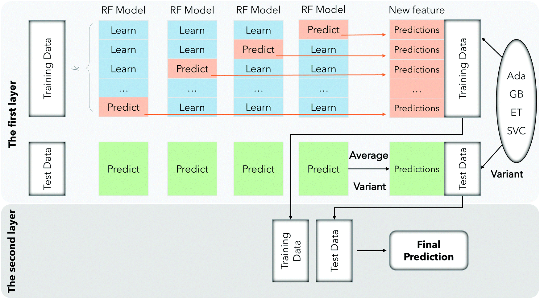 | ||
| Fig. 3 Flowchart of the stacking learning process. | ||
2.6. k-Fold cross validation
The cross-validation method35 is taken because it can obtain as much useful information as possible from limited data, make full use of sample data, and avoid or reduce the occurrence of overfitting situations.Cross validation firstly divides dataset ![[Doublestruck D]](https://www.rsc.org/images/entities/char_e167.gif) into k mutually exclusive subsets of similar size, D = D1∪D2∪…∪Dk, Di∩Dj = ∅ (i ≠ j). Each subset sampling from to get a subset is kept as consistent as possible in the data distribution. Then we use the union of (k − 1) subsets each time as the training set and the remaining subsets as the test set. In this way, k training and testing sets can be obtained, so that k training and testing cycles can be performed, and the average of the k test results is finally returned.
into k mutually exclusive subsets of similar size, D = D1∪D2∪…∪Dk, Di∩Dj = ∅ (i ≠ j). Each subset sampling from to get a subset is kept as consistent as possible in the data distribution. Then we use the union of (k − 1) subsets each time as the training set and the remaining subsets as the test set. In this way, k training and testing sets can be obtained, so that k training and testing cycles can be performed, and the average of the k test results is finally returned.
2.7. Prediction assessment
There are many types of machine learning algorithms in classification, and each algorithm has different mathematical theories and optimization goals. Furthermore, each classification algorithm will perform differently on different training datasets, but there is no classifier whose accuracy can reach 100%. So when a classification task is determined, how to choose a classification algorithm is a problem worth studying. In other words, how to measure the quality of a classifier is what we should talk about. In order to solve this problem, we need a unified set of evaluation criteria.For a binary classification problem,36 the data sample can be divided into true positive (TP), false positive (FP), true negative (TN) and false negative (FN) according to the combination of its real class and the prediction class of the learner.
In this paper, we adopt the following five indicators to test our model. They are Sn (sensitivity), Sp (specificity), Acc (accuracy), Mcc (Matthews correlation coefficient) and the F1-score.
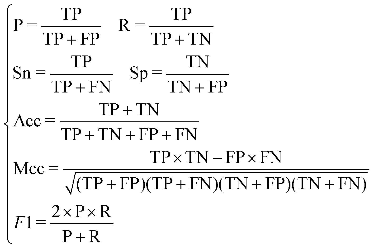 | (14) |
It can be seen from the formula that the recall rate reflects the ability of the classification model to recognize positive examples. The higher the recall rate, the stronger the classifier's ability to recognize positive examples becomes. The precision rate reflects the classifier's ability to distinguish counter examples. The higher the precision rate, the stronger the classifier's ability to distinguish counter examples becomes. The F1-score can be understood as the effect of the classifier when the precision rate and the recall rate reach a balance. Three indicators are considered comprehensively to investigate whether the classification of the classifier has practical significance.
In general, the ROC (Receiver Operating Characteristic) and AUC (Area Under the ROC Curve) are also important indicators to evaluate the prediction. The ROC curve has the TPR (true positive rate) as the x-axis and FPR (false positive rate) as the y-axis, and the class-to-class boundary is defined by a threshold.
The TPR and FPR are defined as follows.
 | (15) |
Then, given a two-classifier model and a threshold, a coordinate position can be determined from the true classification and predicted classification of all data. In this way, the diagonal from coordinates (0,0) to (1,1) divides the ROC space into two regions. The points above the diagonal indicate a classification result that is superior to random classification, and the others below the diagonal represent a poor classification result.
Obviously, for the same classifier, if the given thresholds are different, a different FPR and TPR will be obtained. Therefore, we draw the coordinates of each threshold of the same classifier in the ROC space to form the ROC curve37 of the classifier model. Definitely, when the classification threshold is set to the maximum, all samples are predicted to be negative (counter example), where a point is marked at coordinates (0,0), and, when the classification threshold is set to the minimum, all samples are predicted to be positive (positive example), where a point is marked at coordinates (1,1).
The AUC is the area under the ROC curve, and then we can judge the effectiveness of the classifier.
3. Results and discussion
3.1. Prediction performance
In this study, a novel predictor iDHS-DASTS is developed by the procedures mentioned above.Having determined the test method, another important parameter should also be ascertained, which is the optimal max number of iterations for LASSO. We choose 500, 1000, 1500, 2000, 2500 and 3000 iterations to calculate Acc, Mcc, Sn, Sp, and the F1-score for dataset 1, 2 and 3, respectively, by using a 10-fold cross validation test. From Fig. 4, we can see that Acc obtains the highest value with 93% and the other indicators are the most stable when we choose 1000 iterations for dataset 1. For dataset 2, as shown in Fig. 5, there is nothing ambiguous in the fact that four indicators including Acc, Mcc, Sp and the F1-score are very stable when we choose 1000 iterations. As shown in Fig. 6, Acc, Mcc, Sp and the F1-score all show the best performance when we choose 1000 iterations for dataset 3. Comprehensively, our prediction model becomes less stable when we choose iterations above 1500. In order to make our prediction results more effective and stable, we should choose 1000 iterations to be more reasonable.
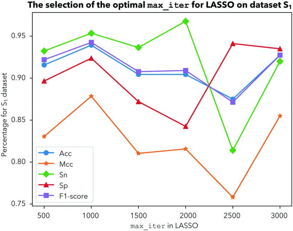 | ||
| Fig. 4 The selection of the optimal max_iter for LASSO on dataset 1. | ||
 | ||
| Fig. 5 The selection of the optimal max_iter for LASSO on dataset 2. | ||
 | ||
| Fig. 6 The selection of the optimal max_iter for LASSO on dataset 3. | ||
As listed in Table 2, the accuracy reaches 92.06%, 91.06% and 90.72% for dataset 1, 2 and 3, respectively. Meanwhile, the values of Sn, Sp, Mcc and the F1-score reach 94.28%, 88.60%, 84.00%, and 92.91%; 87.61%, 94.26%, 82.21%, and 90.41%; and 90.76%, 90.69%, 81.44% and 90.57% for dataset 1, 2 and 3, respectively. We can also obtain the ROC curves of dataset 1, 2 and 3, as shown in Fig. 7, where the AUCs reach 0.91, 0.93 and 0.94. The numerical experiment results indicate that the iDHS-DASTS model achieves excellent and stable performance no matter which dataset it is applied.
1, 2 and 3 by 10-fold cross validation
| Dataset | Acc (%) | Mcc (%) | Sn (%) | Sp (%) | F1-Score (%) |
|---|---|---|---|---|---|
| 1 |
92.06 | 84.00 | 94.28 | 88.60 | 92.91 |
| 2 |
91.06 | 82.21 | 87.61 | 94.26 | 90.41 |
| 3 |
90.72 | 81.44 | 90.76 | 90.69 | 90.57 |
 | ||
| Fig. 7 ROC curve of iDHS-DASTS. | ||
3.2. Performance comparison of different methods
In order to prove the effectiveness of our method, we compare our method with the effectiveness of others. Firstly, we compare different dimensionality reduction methods. In the model of this paper, we use the LASSO dimensionality reduction method. Here we use three other different dimensionality reduction methods to process the data. They are UMAP,38 t-SNE39 and Isomap.40 Through cross-validation, the accuracy of the test set under different dimensionality reduction methods is obtained. In all datasets1, 2 and 3, all indicators of LASSO dimensionality reduction are significantly better than the other three methods, including the fact that the accuracy rate has also been considerably improved.
As is vividly illustrated in Table 3, Acc and Mcc of LASSO reach 92.06% and 84.00% for dataset 1, 91.06% and 82.21% for dataset 2, and 90.72% and 81.44% for dataset 3. Sn and Sp of LASSO also reach 94.28% and 88.60%, 87.61% and 94.26% and 90.76% and 90.69% for dataset 1, 2 and 3, respectively, which are better than UMAP, Isomap and t-SNE. For the two indicators of Sn and Sp, UMAP performs very poorly, showing only 77.69% and 76.98% and 79.20% and 82.35% for dataset 1 and 2, respectively, indicating that the dimensionality reduction effect on the feature vector is not good, and the classification effect is not ideal. The gap between Sn and Sp of the t-SNE dimensionality reduction method is very large, where Sn is 82.03% and 86.29%, and Sp is 64.06% and 69.57%, indicating that the dimensionality reduction method is very unstable. The dimensionality reduction effect of Isomap is more stable, whose accuracy is 86.33%, 84.45% and 83.98%, and Sn and Sp are 87.97% and 89.15%, 84.83% and 80.14%, and 81.89% and 81.17% for dataset 1, 2 and 3, respectively. However, when using Isomap, they all have unsatisfactory results, the Mcc of which is very poor for dataset 1, 2 and 3.
1, 2 and 3 by 10-fold cross validation
| Dataset | Method | Acc (%) | Mcc (%) | Sn (%) | Sp (%) | F1-Score (%) |
|---|---|---|---|---|---|---|
| 1 |
UMAP | 77.34 | 54.68 | 77.69 | 76.98 | 77.69 |
| Isomap | 86.33 | 72.73 | 87.97 | 84.83 | 86.03 | |
| t-SNE | 73.05 | 46.86 | 82.03 | 64.06 | 75.27 | |
| LASSO | 92.06 | 84.00 | 94.28 | 88.60 | 92.91 | |
| 2 |
UMAP | 80.74 | 61.54 | 79.20 | 82.35 | 80.82 |
| Isomap | 84.45 | 69.34 | 89.15 | 80.14 | 84.56 | |
| t-SNE | 78.24 | 56.83 | 86.29 | 69.57 | 80.45 | |
| LASSO | 91.06 | 82.21 | 87.61 | 94.26 | 90.41 | |
| 3 |
UMAP | 83.16 | 66.31 | 83.97 | 82.33 | 83.44 |
| Isomap | 83.98 | 67.66 | 81.89 | 85.71 | 82.25 | |
| t-SNE | 83.37 | 66.82 | 85.09 | 81.82 | 82.90 | |
| LASSO | 90.72 | 81.44 | 90.76 | 90.69 | 90.57 | |
Secondly, when the dataset given by DNA is imbalanced, in order to achieve the best training and classification results, we have adopted SMOTE-Tomek to deal with the data imbalance. Here we take four other methods to deal with the data imbalance or not deal with it. The four methods are Adasyn,41 Boderline-SMOTE,42 SMOTE26 and RandomOverSampling.43 We also try not dealing with the data imbalance to confirm whether our feature extraction is effective. Through cross-validation, the accuracy rate under different methods is obtained.
As shown in Table 4, without over-sampling in our model, Sn and Sp reach 72.22% and 90.67% for dataset 1, 65.96% and 92.41% for dataset 2, and 63.20% and 92.00% for dataset 3. These two indicators are not very good, so it is not appropriate in a stable prediction system. Moreover, Acc and Mcc are pretty good at about 85.78% and 85.94%, 63.27% and 60.71%, and 83.00% and 58.89% before over-sampling, indicating that our feature extraction and dimensionality reduction are effective. As depicted in Table 5, when using Borderline-SMOTE and Adasyn, the accuracy rate is reduced by 10% compared to the original, indicating that the two imbalance treatments are ineffective. However, when using the other two methods, the accuracy of SMOTE is almost the same as before, but, from other indicators, the classifier becomes more stable. The RandomOverSampling method has a certain improvement in various indicators, and the effect is also very good. Obviously, SMOTE-Tomek is a great approach in addressing the data imbalance problem. Acc and Mcc are 6.28% and 5.12%, 20.73% and 21.50%, and 7.72% and 22.55% better than without over-sampling, respectively, for dataset 1, 2 and 3.
| Dataset | Order | Acc (%) | Mcc (%) | Sn (%) | Sp (%) | F1-Score (%) |
|---|---|---|---|---|---|---|
| 1 |
Before | 85.78 | 63.27 | 72.22 | 90.67 | 72.90 |
| After | 92.06 | 84.00 | 94.28 | 88.60 | 92.91 | |
| 2 |
Before | 85.94 | 60.71 | 65.96 | 92.41 | 73.56 |
| After | 91.06 | 82.21 | 87.61 | 94.26 | 90.41 | |
| 3 |
Before | 83.00 | 58.89 | 63.20 | 92.00 | 69.91 |
| After | 90.72 | 81.44 | 90.76 | 90.69 | 90.57 | |
1, 2 and 3 by 10-fold cross validation
| Dataset | Method | Acc (%) | Mcc (%) | Sn (%) | Sp (%) | F1-Score (%) |
|---|---|---|---|---|---|---|
| 1 |
Boderline-SMOTE | 77.68 | 53.67 | 65.96 | 86.15 | 71.26 |
| Adasyn | 74.50 | 49.24 | 72.22 | 77.14 | 75.24 | |
| SMOTE | 84.75 | 69.38 | 79.22 | 84.05 | 83.39 | |
| RandomOverSampling | 86.78 | 73.57 | 90.26 | 82.98 | 87.70 | |
| SMOTE-Tomek | 92.06 | 84.00 | 94.28 | 88.60 | 92.91 | |
| 2 |
Boderline-SMOTE | 73.37 | 47.58 | 72.92 | 78.00 | 72.34 |
| Adasyn | 75.69 | 51.13 | 72.59 | 78.43 | 73.68 | |
| SMOTE | 83.10 | 65.99 | 82.81 | 83.33 | 81.54 | |
| RandomOverSampling | 89.08 | 78.76 | 96.69 | 80.45 | 90.40 | |
| SMOTE-Tomek | 91.06 | 82.21 | 87.61 | 94.26 | 90.41 | |
| 3 |
Boderline-SMOTE | 78.75 | 58.28 | 85.09 | 73.02 | 79.18 |
| Adasyn | 81.14 | 62.80 | 87.54 | 74.73 | 82.27 | |
| SMOTE | 84.29 | 68.55 | 84.37 | 84.19 | 84.67 | |
| RandomOverSampling | 88.39 | 77.39 | 94.64 | 82.14 | 89.08 | |
| SMOTE-Tomek | 90.72 | 81.44 | 90.76 | 90.69 | 90.57 | |
Thirdly, in the case of using LASSO to reduce the dimensionality of the data, we use four classifiers to classify the data set and obtain four group of indicators. The accuracy rate is obtained by cross-validation. The four classifiers are Adaboost,44 random forest,45 support vector machine46 and stacking learning.29 The five indicators are Acc, Mcc, Sn, Sp and the F1-score. As shown in the following Table 6, we can see that the performance of stacking is better than the other three classifier algorithms over the five predictors. Using stacking learning, Acc, Mcc, Sn, Sp and the F1-score significantly improved by 2.68%, 5.18%, 2.78%, 2.33% and 2.98% for dataset 1, and 2.32%, 4.41%, 3.45%, 0.79% and 2.99% for dataset 2 when compared to the best classifier called random forest. For dataset 3, stacking learning has a similar performance to random forest.
1, 2 and 3 by 10-fold cross validation
| Dataset | Classifier | Acc (%) | Mcc (%) | Sn (%) | Sp (%) | F1-Score (%) |
|---|---|---|---|---|---|---|
| 1 |
Adaboost | 86.29 | 73.22 | 80.73 | 92.22 | 85.87 |
| Random forest | 88.92 | 77.79 | 90.40 | 87.29 | 89.50 | |
| SVM | 87.53 | 75.62 | 80.55 | 94.18 | 86.31 | |
| Stacking | 92.06 | 84.00 | 94.28 | 88.60 | 92.91 | |
| 2 |
Adaboost | 85.87 | 72.73 | 79.49 | 93.06 | 85.64 |
| Random forest | 89.28 | 78.56 | 89.73 | 88.83 | 89.49 | |
| SVM | 86.66 | 74.32 | 77.14 | 92.57 | 84.91 | |
| Stacking | 91.06 | 82.21 | 87.61 | 94.26 | 90.41 | |
| 3 |
Adaboost | 89.61 | 79.48 | 93.37 | 85.95 | 89.89 |
| Random forest | 90.78 | 81.59 | 91.71 | 89.89 | 90.71 | |
| SVM | 89.59 | 79.41 | 93.44 | 85.71 | 80.00 | |
| Stacking | 90.72 | 81.44 | 90.76 | 90.69 | 90.57 | |
Finally, in order to more rigorously illustrate the superiority of our model, we selected other models for comparison with our method, and listed various indicators of the different models in classification. In this way, we list the measured values of Acc, Mcc, Sn, Sp and the F1-score for SVM-RevcKmer,47 SVM-PseDNC,20 iDHS-EL,48 iDHS-MFF,49 iDHS-TSA,50 iDHS-DSAMS,50 DHSpred51 and our model iDHS-DASTS in Tables 7 and 8. As shown in Tables 7 and 8, our model represents a significant improvement over the four predictors. The accuracy of iDHS-DASTS model is 6.81%, 8.48%, 5.92%, 5.43%, 4.19%, 2.56% and 4.96% higher than that obtained by the SVM-RevcKmer, SVM-PseDNC, iDHS-EL, iDHS-MFF, iDHS-TSA and iDHS-DSAMS models for dataset 1, respectively, and is 10.49%, 8.06%, 4.92%, 4.12%, 2.12% and 1.41% higher than that obtained by the SVM-RevcKmer, SVM-PseDNC, iDHS-EL, iDHS-MFF, iDHS-TSA, iDHS-DSAMS and DHSpred models for dataset 2, respectively. For dataset 3, as shown in Table 9, among the models testing this dataset, our model has the highest Acc and Mcc, which are 92.51% and 0.85. The accuracy of dataset 3 is 10.75%, 12.4%, 13.9%, 7.4% and 4.03% higher than that obtained by SVM-RevcKmer,47 SVM-PseDNC,20 iDHS-EL,48 Unb-PseTNC52 and pDHS-ELM.53 Furthermore, our model is the most stable method among the five models through the Sn and Sp indicators, whose Sn and Sp both reach about 90% for dataset 1, 2 and 3.
1
| Model | Acc (%) | Mcc | Sn (%) | Sp (%) |
|---|---|---|---|---|
| SVM-RevcKmer | 85.25 | 0.62 | 65.36 | 92.81 |
| SVM-PseDNC | 83.68 | 0.57 | 61.07 | 92.26 |
| iDHS-EL | 86.14 | 0.64 | 64.64 | 94.30 |
| iDHS-MFF | 86.63 | 0.65 | 66.43 | 94.30 |
| iDHS-TSA | 87.87 | 0.76 | 85.91 | 89.84 |
| iDHS-DSAMS | 89.50 | 0.79 | 88.48 | 90.51 |
| DHSpred | 87.10 | 0.66 | 65.50 | 95.20 |
| iDHS-DASTS | 92.06 | 0.84 | 94.28 | 88.60 |
2
| Model | Acc (%) | Mcc | Sn (%) | Sp (%) |
|---|---|---|---|---|
| SVM-RevcKmer | 80.12 | 0.52 | 70.43 | 84.23 |
| SVM-PseDNC | 83.00 | 0.57 | 72.12 | 86.78 |
| iDHS-EL | 86.14 | 0.66 | 64.64 | 94.30 |
| iDHS-MFF | 86.94 | 0.64 | 63.56 | 95.07 |
| iDHS-TSA | 88.94 | 0.78 | 86.48 | 91.41 |
| iDHS-DSAMS | 89.65 | 0.79 | 88.17 | 91.13 |
| iDHS-DASTS | 91.06 | 0.82 | 87.61 | 94.26 |
3
| Model | Acc (%) | Mcc | Sn (%) | Sp (%) |
|---|---|---|---|---|
| SVM-RevcKmer | 81.66 | 0.63 | 82.54 | 79.78 |
| SVM-PseDNC | 80.11 | 0.60 | 81.30 | 78.91 |
| iDHS-EL | 78.61 | 0.57 | 81.24 | 76.11 |
| Unb-PseTNC | 85.11 | 0.70 | 86.48 | 83.74 |
| pDHS-ELM | 88.48 | 0.72 | 89.17 | 87.78 |
| iDHS-DASTS | 92.51 | 0.85 | 93.30 | 91.95 |
4. New independent dataset test
To show the transferability of our model, we validate our prediction model using a new independent dataset. In Section 3, we trained and validated the new and recent dataset, which gained very fantastic results. In this section, we will use our method to train the3 dataset and run separate tests on the 4 dataset, which can solidly prove that our method has great practical results. Through our method, this model testing on the 4 dataset independently has excellent performance. Acc, Mcc, Sn, Sp and the F1-score of this model reached 90.31%, 0.81, 91.90%, 88.59% and 90.78%, respectively.
5. Web-server
In order to improve the practical application value of the model in this paper, we have developed an online web-server for discriminating DNA sequences (Fig. 8). To facilitate the vast majority of experimental scholars, we provide a guide to the use of the web server of this online website. Users do not need to understand the complex mathematical formulas in the prediction process. They only need to input the predicted sequence to get the desired results. | ||
| Fig. 8 The prediction interface of the web-server iDHS-DASTS. | ||
On this website, we explain the source of our dataset in Data, and you can view the use and features of the predictor in Read me, and literature we cited in Citation.
Then you can enter or paste the DNA sequence to be predicted in the center text box. Note that the input format must be in FASTA format. Users can click on Example to view the FASTA format of the standard query given by us. If the query sequence contains irregular characters, an error will be reported and a new entry will be required.
In order to get the query results, the user can also select the data set he needs, and the source of the data set can be found in Data above. Click Submit to submit the DNA sequence you want to predict. Clear will clear the text box content. Of course, the more sequences you enter, the longer it takes to parse them. The web-server for the new predictor is available by clicking the link at http://www.xdu-duan.cn/.
6. Conclusion
This study aimed to develop a classifier for predicting DHSs and non-DHSs. Considering the importance of the global and mutual information in a given sequence, a novel feature extraction method called iDHS-DASTS is constructed in our study. In the feature extraction method, we perform a recombination based on the physicochemical properties, instead of a simple trade-off of the original variables. Meanwhile, compared to others, iDHS-DASTS focuses more on cross-correlation and spatial autocorrelation of the sequence. We adopt the Least Absolute Shrinkage and Selection Operator (LASSO) to reduce the dimensions. In addition, it is of great use to deal with imbalanced datasets1, 2 and 3via SMOTE-Tomek. By balancing the datasets, it can be more accurate for the classifier to find the potential connections between the feature and the DHSs. Finally, in the process of constructing the classifier, stacking learning decreases the possibility of overfitting and greatly reduces the instability of the trained classifier due to its random sampling. Furthermore, to show the transferability of our model, we validate our prediction model using a new independent dataset 4. More significantly, in order to increase its practical value, we created a website http://www.xdu-duan.cn to provide a iDHS-DASTS web-server. Users do not need to understand the complex formulas in the prediction process, just input the predicted sequence, and can easily obtain the forecast results.
Availability of data and materials
Experimental datasets are available at http://www.xdu-duan.cn.Conflicts of interest
The authors declare that there is no conflict of interest regarding the publication of this paper.Acknowledgements
This work was supported by the National Natural Science Foundation of China (No. 11601407), and the Natural Science Basic Research Plan in Shaanxi Province of China (No. 2018JM1037, 2019JQ-279).References
- C. Wu, P. M. Bingham, K. J. Livak, R. Holmgren and S. C. R. Elgin, The chromatin structure of specific genes: I. Evidence for higher order domains of defined DNA sequence, Cell, 1979, 16(4), 797–806 CrossRef CAS.
- D. S. Gross and W. T. Garrard, Nuclease Hypersensitive Sites in Chromatin, Annu. Rev. Biochem., 1988, 57(1), 159–197 CrossRef CAS.
- G. Felsenfeld, Chromatin as an essential part of the transcriptional mechanim, Nature, 1988, 355(6357), 219–224 CrossRef.
- G. Felsenfeld and M. Groudine, Controlling the double helix, Nature, 2003, 421(6921), 448–453 CrossRef.
- G. E. Crawford, I. Holt, J. R. R. Whittle, B. D. Webb, D. Tai, S. Davis, E. H. Margulies, Y. Chen, J. A. Bernat and D. Ginsburg, et al., Genome-wide mapping of dnase hypersensitive sites using massively parallel signature sequencing (mpss), Genome Res., 2005, 16(1), 123–131 CrossRef.
- N. W. Stafford, K. Scott, T. Robert, Y. Man and S. John, Predicting the in vivo signature of human gene regulatory sequences, Bioinformatics, 2005, i338–i343 Search PubMed.
- X. Zhou, Z. Li, Z. Dai and X. Zou, Predicting methylation status of human DNA sequences by pseudo-trinucleotide composition, Talanta, 2011, 85(2), 0–1147 CrossRef CAS.
- C. Wei, P. M. Feng, L. Hao and C. Kuo-Chen, iRSpot-PseDNC: identify recombination spots with pseudo dinucleotide composition, Nucleic Acids Res., 2013, 6, 6 Search PubMed.
- W. R. Qiu, X. Xiao and K.-C. Chou, iRSpot-TNCPseAAC: Identify Recombination Spots with Trinucleotide Composition and Pseudo Amino Acid Components, Int. J. Mol. Sci., 2014, 15(2), 1746–1766 CrossRef.
- S. Li, E. J. Harner and D. A. Adjeroh, Random KNN feature selection – a fast and stable alternative to Random Forests, BMC Bioinf., 2011, 12(1), 450 CrossRef.
- O. Sarrafzadeh and A. M. Dehnavi, Nucleus and cytoplasm segmentation in microscopic images using K-means clustering and region growing, Adv. Biomed. Res., 2015, 4, 174 Search PubMed.
- Z. Yang, W. W. S. Wong and N. Rasmus, Bayes Empirical Bayes Inference of Amino Acid Sites Under Positive Selection, Mol. Biol. Evol., 2005, 4, 4 Search PubMed.
- K. K. Kandaswamy, K. C. Chou, T. Martinetz, S. Möller, P. N. Suganthan, S. Sridharan and G. Pugalenthi, AFP-Pred: A random forest approach for predicting antifreeze proteins from sequence-derived properties, J. Theor. Biol., 2011, 270(1), 56–62 CrossRef CAS.
- Y. Cai, P. Ricardo, C. Jen and K. Chou, Application of svm to predict membrane protein types, J. Theor. Biol., 2004, 226(4), 373–376 CrossRef CAS.
- B. Gu, V. S. Sheng and A. Robust, Regularization Path Algorithm for ν-Support Vector Classification, IEEE Trans. Neural Networks Learn. Syst., 2017, 28(5), 1241–1248 Search PubMed.
- B. Gu, V. S. Sheng, K. Y. Tay, W. Romano and S. Li, Incremental Support Vector Learning for Ordinal Regression, IEEE Trans. Neural Networks Learn. Syst., 2014, 26(7), 1403–1416 Search PubMed.
- T. W. Smith and S. A. Colby, Teaching for Deep Learning, Clearing House A Journal of Educational Strategies Issues & Ideas, 2007, 80(5), 205–210 Search PubMed.
- Y. Park and M. Kellis, Deep learning for regulatory genomics, Nat. Biotechnol., 2015, 33(8), 825–826 CrossRef CAS.
- M. Spencer, J. Eickholt and J. Cheng, A Deep Learning Network Approach to ab initio Protein Secondary Structure Prediction, IEEE/ACM Trans. Comput. Biol. Bioinform., 2015, 12(1), 103–112 CAS.
- P. Feng, N. Jiang and N. Liu, Prediction of DNase I Hypersensitive Sites by Using Pseudo Nucleotide Compositions, Sci. World J., 2014, 2014, 1–4 Search PubMed.
- L. Fu, B. Niu, Z. Zhu, S. Wu and W. Li, Cd-hit: accelerated for clustering the next-generation sequencing data, Bioinformatics, 2012, 23, 3150–3152 CrossRef.
- C.-J. Zhang, H. Tang, W.-C. Li, H. Lin, W. Chen and K.-C. Chou, iori-human: identify human origin of replication by incorporating dinucleotide physicochemical properties into pseudo nucleotide composition, Oncotarget, 2016, 7(43), 69783 CrossRef.
- T. Lee, P. Chao, H. Ting, L. Chang, Y. Huang, J. Wu, H. Wang, M. Horng, C. Chang and J. Lan, et al., Using Multivariate Regression Model with Least Absolute Shrinkage and Selection Operator (LASSO) to Predict the Incidence of Xerostomia after Intensity-Modulated Radiotherapy for Head and Neck Cancer, PLoS One, 2014, 9(2), e89700 CrossRef.
- T. T. Wu and K. Lange, Coordinate descent algorithms for lasso penalized regression, Ann. Appl. Stat., 2008, 2(1), 224–244 CrossRef.
- N. Simon, J. H. Friedman, T. Hastie and R. Tibshirani, A Sparse-Group Lasso, J. Comput. Graph. Stat., 2013, 22(2), 231–245 CrossRef.
- N. V. Chawla, K. W. Bowyer, L. O. Hall and W. P. Kegelmeyer, SMOTE: synthetic minority over-sampling technique, J. Artif. Intell. Res., 2002, 16, 321–357 CrossRef.
- M. Kubat and S. Matwin, Addressing the Curse of Imbalanced Training Sets: One-Sided Selection, International Conference on Machine Learning, 1997, pp. 179–186.
- W. Lei, Effective prediction of three common diseases by combining SMOTE with Tomek links technique for imbalanced medical data, in: IEEE International Conference of Online Analysis & Computing Science, 2016.
- T. G. Dietterich, Ensemble learning, The Handbook of Brain Theory and Neural Networks, 2002, vol. 2, pp. 110–125 Search PubMed.
- P. O. Gislason, J. A. Benediktsson and J. R. Sveinsson, Random forests for land cover classification, Pattern Recognit. Lett., 2006, 27(4), 294–300 CrossRef.
- X. Li, L. Wang and E. Sung, AdaBoost with SVM-based component classifiers, Eng. Appl. Artif. Intell., 2008, 21(5), 785–795 CrossRef.
- N. Alexey and K. Alois, Gradient boosting machines, a tutorial, Front. Neurorobotics, 2013, 7, 21 Search PubMed.
- P. Geurts, D. Ernst and L. Wehenkel, Extremely randomized trees, Mach. Learn., 2006, 63(1), 3–42 CrossRef.
- J. A. K. SuykensJ, Vandewalle, Least Squares Support Vector Machine Classifiers, Neural Process. Lett., 1999, 9(3), 293–300 CrossRef.
- J. Shao, Linear Model Selection by Cross-validation, J. Am. Stat. Assoc., 1993, 88(422), 486–494 CrossRef.
- J. T. Townsend, Theoretical analysis of an alphabet confusion matrix, Atten. Percept. Psychophys., 1971, 9(1), 40–50 CrossRef.
- K. Hajian-Tilaki, Receiver Operating Characteristic (ROC) Curve Analysis for Medical Diagnostic Test Evaluation, Caspian J. Intern. Med., 2013, 4(2), 627–635 Search PubMed.
- L. McInnes, J. Healy and J. Melville, UMAP: Uniform manifold approximation and projection for dimension reduction, 2018, arXiv preprint arXiv:1802.03426.
- L. van der Maaten and G. Hinton, Visualizing data using t-SNE, J. Mach. Learn. Res., 2008, 9, 2579–2605 Search PubMed.
- G. J. Bowen, Z. Liu, H. B. V. Zanden, Z. Lan and G. Takahashi, Geographic assignment with stable isotopes in IsoMAP, Methods Ecol. Evol., 2014, 5(3), 201–206 CrossRef.
- H. He, B. Yang, E. A. Garcia and S. Li, ADASYN: Adaptive Synthetic Sampling Approach for Imbalanced Learning, Neural Networks, 2008. IJCNN 2008. (IEEE World Congress on Computational Intelligence). IEEE International Joint Conference on, 2008, pp. 1322–1328.
- H. Han, W. Y. Wang and B. H. Mao, Borderline-SMOTE: A New Over-Sampling Method in Imbalanced Data Sets Learning, International conference on intelligent computing, Springer, Berlin, Heidelberg, 2005, pp. 878–887.
- A. Moreo, A. Esuli and F. Sebastiani, Distributional Random Oversampling for Imbalanced Text Classification, International ACM Sigir Conference on Research and Development in Information Retrieval, 2016, pp. 805–808.
- Y. Lu, W. Qu, G. Shan and C. Zhang, DELTA: A Distal Enhancer Locating Tool Based on AdaBoost Algorithm and Shape Features of Chromatin Modifications, PLoS One, 2015, 10(6), e0130622 CrossRef.
- L. R. Verónica, L. S. Maria and S. Luis, Distinguishing between productive and abortive promoters using a random forest classifier in Mycoplasma pneumoniae, Nucleic Acids Res., 2015, 7, 7 Search PubMed.
- N. Shibuya, B. T. Nukala, A. I. Rodriguez, J. Tsay, T. Q. Nguyen, S. Zupancic and D. Y. C. Lie, A real-time fall detection system using a wearable gait analysis sensor and a Support Vector Machine (SVM) classifier, in: 2015 Eighth International Conference on Mobile Computing and Ubiquitous Networking (ICMU), 2015.
- W. S. Noble, S. Kuehn, R. E. Thurman, M. Yu and J. A. Stamatoyannopoulos, Predicting the in vivo signature of human gene regulatory sequences, Bioinformatics, 2005, 21(1), 338–343 CrossRef.
- B. Liu, R. Long and K. Chou, iDHS-EL: identifying DNase I hypersensitive sites by fusing three different modes of pseudo nucleotide composition into an ensemble learning framework, Bioinformatics, 2016, 32(16), 2411–2418 CrossRef.
- Y. Liang and S. Zhang, Identifying DNase I hypersensitive sites using multi-features fusion and F-score features selection via Chou's 5-steps rule, Biophys. Chem., 2019, 253, 106227 CrossRef CAS.
- S. Zhang, Q. Yu, H. He, F. Zhu, P. Wu, L. Gu and S. Jiang, iDHS-DSAMS: Identifying DNase I hypersensitive sites based on the dinucleotide property matrix and ensemble bagged tree, Genomics, 2020, 112(2), 1282–1289 CrossRef CAS.
- B. Manavalan, T. H. Shin and G. Lee, Dhspred: support-vector-machine-based human dnase i hypersensitive sites prediction using the optimal features selected by random forest, Oncotarget, 2018, 9(2), 1944–1956 CrossRef.
- M. Kabir and D.-J. Yu, Predicting dnase i hypersensitive sites via un-biased pseudo trinucleotide composition, Chemom. Intell. Lab. Syst., 2017, 167, 78–84 CrossRef CAS.
- S. Zhang, M. Chang, Z. Zhou, X. Dai and Z. Xu, pdhs-elm: Computational predictor for plant dnase i hypersensitive sites based on extreme learning machines, Mol. Genet. Genomics, 2018, 293(4), 1035–1049 CrossRef CAS.
Footnote |
| † Electronic supplementary information (ESI) available. See DOI: 10.1039/d0mo00115e |
| This journal is © The Royal Society of Chemistry 2021 |