
Towards a machine learned thermodynamics: exploration of free energy landscapes in molecular fluids, biological systems and for gas storage and separation in metal–organic frameworks
Caroline
Desgranges
 ab and
Jerome
Delhommelle
*ab
ab and
Jerome
Delhommelle
*ab
aDepartment of Chemistry & Molecular Simulation of NonEquilibrium Processes (MSNEP), Tech Accelerator, University of North Dakota, Suite 2300, USA. E-mail: jerome.delhommelle@und.edu
bDepartment of Chemistry, New York University, USA
First published on 23rd November 2020
Abstract
In this review, we examine how machine learning (ML) can build on molecular simulation (MS) algorithms to advance tremendously our ability to predict the thermodynamic properties of a wide range of systems. The key thermodynamic properties that govern the evolution of a system and the outcome of a process include the entropy, the Helmholtz and the Gibbs free energy. However, their determination through advanced molecular simulation algorithms has remained challenging, since such methods are extremely computationally intensive. Combining MS with ML provides a solution that overcomes such challenges and, in turn, accelerates discovery through the rapid prediction of free energies. After presenting a brief overview of combined MS–ML protocols, we review how these approaches allow for the accurate prediction of these thermodynamic functions and, more broadly, of free energy landscapes for molecular and biological systems. We then discuss extensions of this approach to systems relevant to energy and environmental applications, i.e. gas storage and separation in nanoporous materials, such as metal–organic frameworks and covalent organic frameworks. We finally show in the last part of the review how ML models can suggest new ways to explore free energy landscapes, identify novel pathways and provide new insight into assembly processes.
Design, System, ApplicationMachine learning (ML) has emerged as a remarkably efficient predictive tool for thermodynamic properties, and has the potential to accelerate considerably the screening of molecules, biological systems or of nanoporous materials for specific applications. To achieve this, ML models are optimized using training datasets generated through high-resolution molecular simulations (MS). Here we focus on free energy and examine how combined MS–ML approaches shed light on the properties of molecular systems, leading to the rapid determination, e.g. of their phase behavior. We also discuss how such methods can be extended to biological systems, with the identification, for instance, of the folded states of proteins, and to fluids confined in nanoporous materials, with the fast evaluation of the free energy costs involved in the gas storage and separation of energy-related molecules, such as hydrogen or methane, and of environmental contaminants. These approaches can also be leveraged to explore free energy landscapes, leading to the elucidation of novel pathways for a wide range of activated processes. |
1 Introduction
In recent years, machine learning (ML) has emerged as an extremely useful tool to explore and predict complex phenomena.1–16 Data-driven methods yield excellent results when applied to the parametrization of new force fields and coarse-grained models17–27 or to facilitate the exploration of the chemical space in inverse design methods.28–30 ML methods have also been applied in recent years to the reconstruction of complex high-dimensional potential energy surfaces31–34 and to the prediction of thermodynamic and kinetic properties.35–37 This considerably accelerates the determination of the key properties for these systems, since their computation via conventional molecular simulation methods often requires an extensive sampling of the phase space, i.e. performing simulations over very large time-scales and length-scales that quickly become extremely computationally intensive. ML can also provide new insights into assembly processes38–40 and yield predictive models for heterogeneous catalysis.29,41 Artificial neural networks have also been shown to provide access to free energy landscapes that are difficult to compute. Examples include processes that involve transitions from one state to another, a task for which rare event sampling and enhanced sampling simulations are required.42–46 Similarly, ML models can be leveraged to predict adsorption isotherms, adsorption free energies, catalytic activities on nanoclusters surfaces47 and as a way to accelerate considerably materials discovery. ML algorithms and ensemble learning models yield new routes to quickly screen potential candidates for application in gas storage and separation.48–50 ML predictions on gas adsorption capabilities can also be carried out on the basis of crystal designs of materials such as metal–organic frameworks (MOFs) and covalent organic frameworks (COFs) at operating conditions.51–54 Such predictions, in turn, also suggest new ways of tailoring novel materials with enhanced adsorption properties.55–58In this review, we focus on how ML can help us predict the key thermodynamic properties that govern the evolution and outcome of a system. This includes the Helmholtz free energy for systems with a constant volume and temperature, the Gibbs free energy when the temperature and pressure are held constant or the entropy in the case of isolated systems. Many thermodynamic properties can be readily measured in experiments, or calculated during the course of molecular simulation (MS) runs. This is the case, e.g., of the volume, temperature, pressure, internal energy or enthalpy of a system. On the other hand, thermodynamic functions like the entropy and the Helmholtz or Gibbs free energy cannot be evaluated directly, as they require information on all the microstates available to the system. This has led to the invention of novel MS algorithms that achieve an extensive sampling of all possible configurations of the system. The next section of this review discusses several of these strategies, as these MS algorithms provide access to free energies and free energy landscapes that serve as the starting point for the construction of ML models. We briefly discuss how MS data can be used to train ML models on the example of a well-established and widely used deep learning algorithm, know as artificial neural networks (ANNs).1,59–63 We then show how MS–ML approaches lead to accelerated predictions of free energies and extend the discussion to other ML methods for free energy predictions. Then, we examine several applications of ML models to molecular and biological systems, before turning to applications in the field of gas storage and separation. We finally discuss how MS–ML approaches can be leveraged to unravel new pathways for assembly processes and provide new insights into such processes.
2 Building ML models for thermodynamics
2.1 Datasets generation
The first step consists in the generation of data on the free energy for the system under study. This data will then be used to train and teach the ML models and allow them to learn the thermodynamics, and free energy landscape, of the system. To achieve the evaluation of free energy, MS algorithms rely on determining free energy differences along a thermodynamic path connecting the system actually studied and a reference state for the system. Free energy differences can be indeed obtained by thermodynamic integration64–68 along paths that connect, for instance, a liquid to an ideal gas or a “real” crystal to an Einstein crystal.69,70 For instance, considering a crystal for a given number of atoms N, volume V and temperature T, the Helmholtz free energy difference ΔF is given by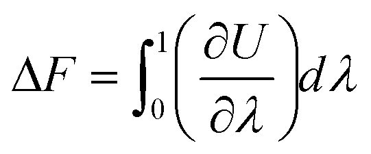 | (1) |
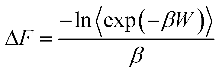
Another class of methods, known as enhanced sampling simulations, is required when the system has to overcome large free energy barriers along this thermodynamic path. This is, e.g., the case when a molecular system undergoes a phase transition through the nucleation of a new phase, or when a protein undergoes a conformational change or folding event. Examples of enhanced sampling methods include the umbrella sampling method71–73 and metadynamics.74–77 In such cases, an external potential energy ϒ may be added to the system to bolster the sampling of configurations of high free energy, which would not be observed in the absence of the external potential. This potential is often taken to be a harmonic function of a reaction coordinate ϕ that spans the thermodynamic path. Statistics for P(ϕ), the probability of observing configurations with a given value of ϕ, are collected over the course of MS runs. The free energy profile is then obtained by subtracting the external potential energy and by recognizing that the free energy along the profile can be calculated from –kBT![[thin space (1/6-em)]](https://www.rsc.org/images/entities/char_2009.gif) lnP(ϕ). For more details on the derivation of the free energy using the umbrella sampling method, we refer the readers to the excellent references by Torrie and Valleau,71 as well as recent work by Kästner.78 More specifically, examining a process for a given number of atoms N, pressure P and temperature T, the Gibbs free energy difference can be calculated along a path spanned by the reaction coordinate ϕ. In this case, ΔG is given by
lnP(ϕ). For more details on the derivation of the free energy using the umbrella sampling method, we refer the readers to the excellent references by Torrie and Valleau,71 as well as recent work by Kästner.78 More specifically, examining a process for a given number of atoms N, pressure P and temperature T, the Gibbs free energy difference can be calculated along a path spanned by the reaction coordinate ϕ. In this case, ΔG is given by
| ΔG(ϕ) = −kBTlnP(ϕ) − ϒ(ϕ) | (2) |
 | (3) |
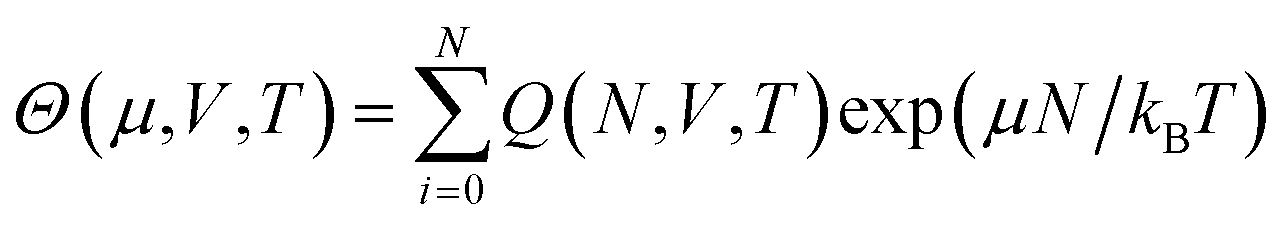
Free energy can also be determined through another broad class of simulation approaches known as flat histogram methods.107–113 Such approaches rely on an extensive sampling of all possible configurations of the system, with the aim of determining the density of states g(E) of a given system. One such approach, the Wang–Landau sampling method,107,114–116 was initially implemented in the microcanonical (N, V, E) ensemble and consists in performing a random walk in energy space with a probability proportional to the reciprocal of the density of states 1/g(E). At the start of the simulation, g(E) is unknown. Its value is initially set to g(E) = 1 for all E, with g(E) dynamically updated during the simulations until a flat histogram for the number of visits of each E interval is obtained. This method thus yields g(E) up to a multiplicative constant, It can also be extended to various ensembles including the canonical (N, V, T) ensemble109 or the isothermal–isobaric (N, P, T) ensemble110,111,117–120 to determine the corresponding partition functions up to a multiplicative factor. In some cases, the multiplicative factor can be determined, and exact values for the partition functions, and thus for the free energy, can be obtained. This has been achieved with the expanded Wang–Landau (EWL) simulation method112,121–124 that performs an extensive sampling of the grand-canonical (μ, V, T) ensemble.125–128 In this case, the algorithm yields Θ(μ, V, T), the partition function for the grand-canonical ensemble, as well as the underlying canonical partition function Q(N, V, T), as given by
 | (4) |
| F(N,V,T) = −kBTlnQ(N,V,T) | (5) |
2.2 Model training and validation
The second step consists in using the simulation data to train a ML model. ANNs have emerged as highly versatile deep learning algorithms and are popular choices for ML models.1,59–63 Thus, to illustrate how ML models can be built to interpolate between, and extrapolate beyond, the conditions covered by the simulation data, we consider an ANN as outlined in the schematic blueprint of Fig. 1 that summarizes how ML models can be built from the simulation data. Popular approaches rely on the training of neural networks with a feed-forward structure and use an optimization algorithm back-propagation error calculation136 to optimize the weights, or contributions made by each neuron, to the overall result. As an example, we consider an ANN with 4 layers. The first layer is an input layer, with a series of input neurons that correspond to the key parameters or descriptors for the system. There can be as many input neurons Gi (i = 1, 2,…) as desired. These can be thermodynamic variables, such as T or P, or geometric parameters, such as, for instance, dihedral angles in the case of free energy landscapes for protein folding. The next two layers are known as hidden layers, and contain variable numbers of neurons h1 and h2. The last layer is termed the output layer, with output neurons corresponding to the properties the ML model aims to predict including, e.g., the free energy, partition function137,138 or any other property of interest. If one of the output neurons is for the ML-predicted free energy FML, the ML model provides the following analytic equation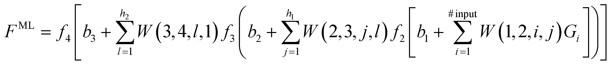 | (6) |
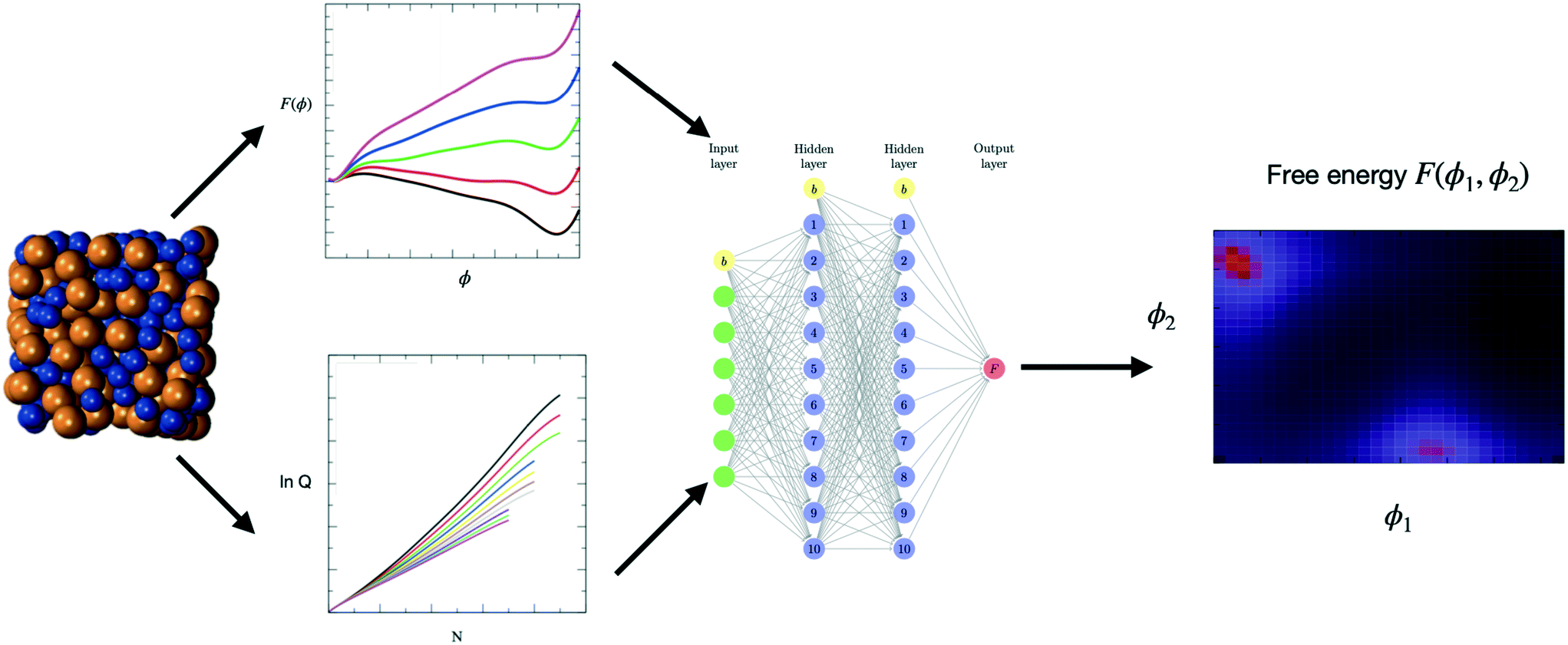 | ||
| Fig. 1 Schematic blueprint for a combined MS–ML protocol. Molecular simulations (first panel on the left) can be carried out to generate free energy profiles (top of second panel) or partition functions (bottom of second panel). The simulation data is then used to train a ML model (here the ANN of the third panel) and lead to the prediction of free energies for conditions outside of those covered by the simulation data (here a 3D plot of F(ϕ1, ϕ2) in the (ϕ1, ϕ2) plane) and of free energy minima as shown by the bright regions on the plot (fourth panel on the right). | ||
The ANN is trained by minimizing an error function that quantifies the difference between the free energy from the simulation data Fi and the free energy predicted by the ML model FMLi
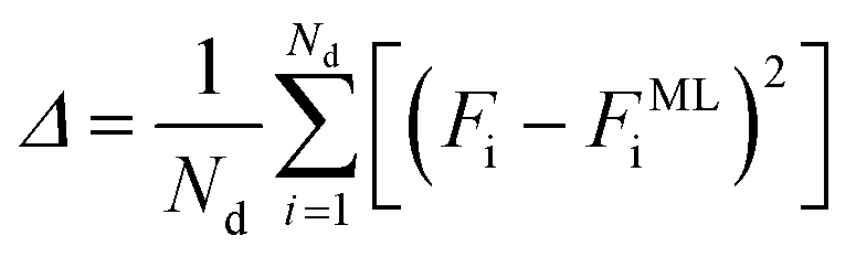 | (7) |
Weights can be adjusted after each forward pass, using an optimization algorithm during the backward pass. The process is then repeated iteratively until additional iterations do not lead to a change in the accuracy of the predictions. The back-propagation algorithm is often used to optimize all weights once per iteration, leading to the following equation
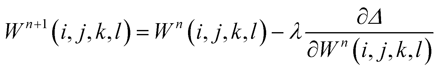 | (8) |
The simulation data is generally split between a training set for the optimization of the ANN weights and a hold-out set for validation purposes. It is often useful to carry out calculations of root-mean square errors for both the training and hold-out sets. Both RMSEs are helpful in determining the accuracy of the ML model, but also to assess if any underfitting or overfitting of the simulation data takes place. For instance, obtaining a small RMSE for the ML model with respect to the training dataset and a large RMSE with respect to the hold-out/validation dataset can be indicative of an overfit. On the other hand, having RMSEs that are small and of the same order for both datasets shows that the ML model performs very well.
The size of the datasets used to train and validate the ML model depends on several factors, such as, e.g., the complexity of the data to be modeled and the type, and architecture, of the ML model. Preliminary tests are often performed to assess how the performance of a ML model scales with the dataset size. In practice, this can be achieved through the use of a learning curve, or training curve, that captures how the performance of the ML model, measured through a training and a validation score, improves as the size of the training dataset is increased. This tool is especially useful in determining if the ML model gives rise to any underfitting or overfitting of the data, or if the ML model performs very well for the task at hand. Typical sizes for datasets used in the training of ML models for the prediction of free energy surfaces include of the order of 104–105 data points.139 A set of 104 data points is typical for datasets for partition functions used in the training of ML models.137
The preparation of the datasets is also key to the optimization of the ML model. In order to reduce bias, it may be advantageous to adopt an ensemble learning approach, in which the ML predictions are averaged over several ANNs with different W matrices.50,140 The k members of an ensemble of ANNs can be obtained through several strategies. One such strategy is known as k-fold cross-validation. In this case, a collection of ANNs with exactly the same architecture is trained on randomized subsets of the training dataset, and the k models are then used as the members of an ensemble.141 Another strategy is known as the bootstrap aggregation (bagging)142 approach with replacement. The idea there is to generate k training subsets with different sample densities, with the aim of emphasizing the weight of different parts of the dataset in the optimization process. Alternatively, a diversity approach can be adopted by using different ANN architectures and varying the number of neurons in the hidden layers.143
Several other ML methods can also be applied to build and predict free energy surfaces from the simulation data. Such methods include Bayesian inference,144–150 Gaussian progress regression,151 kernel ridge regression, support vector machines, weighted neighbor schemes,139 dimensionality reduction as well as transfer learning and reinforcement learning.152 We finally add that ML models perform extremely well when they are used to make predictions for conditions that lie between those covered in the training datasets. Extrapolations beyond the range of conditions included in the datasets can often be carried out reliably, provided that the systems exhibit similar properties, e.g. similar phases for the predictions of fluid properties.50,137 However, as a general rule, extrapolations using a ML model should be carried out with caution, especially if the system undergoes dramatic changes (e.g. conformational changes for a biomolecule) that are outside the range of possibilities considered in the training set. In that case, direct extrapolations may yield to inaccurate predictions.
3 ML-predictions of free energy landscapes for molecular and biological systems
The introduction of computer simulations in science has advanced tremendously our understanding of the mechanisms that take place at the microscopic level in molecular and biological systems. The ability of simulations to model increasingly complex systems and to bridge between different length scales and time scales via multiscale methods has been instrumental to the unraveling of many chemical processes.153–155 As simulations have taken into account finer and finer details of the intermolecular interactions, leading, in turn, to increasingly accurate results, CPU and GPU times have become more and more significant. In order to overcome such challenges, an increasing number of researchers implement ML approaches to fast-track the simulations156 and accelerate chemical discovery.157 ML methods have been used to screen materials, providing excellent starting points for the computational optimization of catalysts and for the discovery of new trends and behavior.158,159 They have also been employed to predict the properties of molecules and crystals, with the development, e.g., of novel ML models based on graph networks to obtain the formation energies, band gaps and elastic moduli of crystals with an accuracy comparable to density functional theory when very large dataset are used for training purposes.160ML methods can also be leveraged to predict the free energy of molecular and biological systems. This can be achieved, for instance, by providing a way to extrapolate the simulation data beyond the range of conditions covered by the simulations.44,137,138,148 Such protocols have been applied to molecular, polymeric and biological systems, which present stringent tests for the methods as the energy landscapes are often rugged. A variety of methods have been developed to tackle such systems. For instance, nonlinear machine techniques have been used to recover single molecule free energy landscapes from molecular simulations.42 In this case, the diffusion map nonlinear machine learning technique is used to understand the relation between changes in external conditions, or in molecular chemistry, and the free energy landscape, with applications to the n-eicosane chain and to a family of polyglutamate-derivative homopeptides, In the latter case, the helical stability-side chain length interdependence and the critical side chain length for the helix–coil transition were identified.
Artificial neural networks can also be employed to learn free energy landscapes through the use of adaptive biasing potentials and of Bayesian regularization to increasing the robustness of the approach to hyperparameters and overfitting.148 In this case, Bayesian regularization penalizes network weights and auto-regulates the number of effective parameters in the network. Alternatively, ANNs can be used to generate the free energy landscapes for the conformational equilibria in complex molecular systems.44 Starting from free energy data obtained from enhanced-sampling molecular simulations, ANNs are trained to represent the free energy surfaces of the alanine di- and tripeptides in the gas phase. Another approach consists in using ANNs to predict the partition function of molecular fluids137 and, thus, to gain access to all properties of the system, including the free energy as outlined in the previous section. Using simulation data for the partition functions obtained from expanded Wang–Landau simulations, ANNs are trained to predict the free energy and the phase behavior of molecules over a wide range of conditions. In the case of higher-dimensional surfaces, such as in the case of multicomponent mixtures,138 the determination of free energy and of the locus for phase transitions can be greatly accelerated by the combined use of ML and MS methods, with combined approaches only requiring about 20% of the computational cost involved in a conventional flat-histogram MS approach to elucidate fully the free energy landscape and phase behavior. In recent work, alternative strategies, including kernel ridge regression, support vector machines and weighted neighbor schemes have been used to learn free energy landscapes and generate accurate ensemble averages for the observable properties of oligopeptides in the gas phase, as well as in an aqueous solution.139
In addition to providing predictions for the free energy, ML models can also be used to gain access to the kinetics of processes.161 As the system under study becomes more complex, its underlying kinetic properties become increasingly challenging to determine and interpret. This is most particularly the case of proteins, and the implementation of dimensionality reduction, transfer learning and reinforcement learning is starting to show promising results.152 ML models can also be used to compute the solvation free energy. Approaches using a global optimization procedure have been developed to identify low-energy molecular clusters for different numbers of explicit solvent molecules,162 and sketch maps and nonlinear dimensionality reduction algorithms can be leveraged to quantify similarities between solute environments in microsolvated clusters. Hydration free energies have also been determined by combining alchemical free energy calculations with ML, leading to the computation of highly accurate absolute hydration free energies.163 Such approaches that combine free energy methods with machine learning show great promise, most particularly for the study of systems of increasing complexity, including the determination of the free energy of protein–ligand binding for drug design and drug development,164–167 and in the membrane transport cycle.168
4 ML thermodynamics of adsorption
The development of ML models for adsorption processes has drawn considerable interest in recent years. Several types of applications can indeed be explored through such models. This includes catalysis, with the determination of adsorption energies of molecules such as hydrogen47 on metal surfaces and metal nanoalloys through, e.g., the combination of ML with density functional theory (DFT) methods.56,169–178 ML predictions for the free energy of adsorbed phases, and the corresponding surface phase diagram over a wide range of coverages and adsorbates, has been carried out with a Gaussian process regression model on IrO2 and MoS2 surfaces for applications in electrocatalysis.179Another broad class of applications deals with the study of porous nanomaterials, such as metal–organic frameworks (MOFs) and covalent organic frameworks (COFs).58,180 These materials are candidates for gas storage and separation in energy-related processes48 and in environmental processes. Examples of systems for such applications include, among others, the storage of methane181 or hydrogen for energy applications, as well as the sequestration182 of CO2 or of polycyclic aromatic hydrocarbons (PAHs)183 for environmental applications. In these systems, a gas phase is in thermodynamic equilibrium with the gas adsorbed inside the COF or MOF, which means that the two phases share the same molar Gibbs free energy or chemical potential (as well as the same temperature). In this case, the relation between free energy and the properties of the adsorbed phase can be obtained through grand canonical Monte Carlo (GCMC) simulations. These simulations provide access to, for instance, the amount of molecules adsorbed in the framework as a function of the chemical potential, or to the selectivity towards a specific molecule in the case of the adsorption of mixtures.
ML can be combined with GCMC simulations to screen nanoporous materials and identify the best candidates to reach volumetric targets for practical applications. For instance, hydrogen storage is a major challenge for hydrogen use in contemporary applications as a fuel for automobiles and vehicular applications. Here, the idea is to have sufficiently densified hydrogen at a moderate pressure to power vehicles. Nanoporous materials such as, e.g., MOFs and COFs are novel materials that effectively alleviate the issue of storage pressure.184–188 Recent studies have started to leverage ML methods to model and predict adsorption in such systems. The combined use of grand canonical Monte Carlo simulations and of neural networks53 has led to the proposal of new crystal designs, and their performance has been assessed by determining hydrogen storage capabilities for various pressure swing conditions.51 Gaussian process regression has also been employed to predict hydrogen adsorption in nanoporous materials using the CoRE-MOF database.189 Furthermore, strategies combining Monte Carlo approaches with ML methods have yielded very promising results, in their efficiency in screening materials as candidates for the storage of several gases, including methane,190 carbon dioxide, hydrogen and hydrogen sulfide.191
Another application of ML to adsorption phenomena is the ‘in silico’ discovery of novel materials for carbon capture. Genetic algorithms have been employed to compute interactions between adsorbates like CO2 and the framework, and to derive accurate force field parameters for molecular simulations.192 Moreover, deep learning has allowed for the improved assessment of the importance of textural properties in porous carbons for CO2 adsorption. In this case, ANNs are trained as a generative model to shed light on this interdependence and, as a result, to guide the development of the next generation of porous carbon materials.57
ML can also be leveraged to tackle the adsorption of multicomponent gas mixtures. In this case, having multiple components in the adsorbate increases the dimension of the parameter space that needs to be studied. This is indeed necessary to quantify the dependence of the selectivity towards the adsorption of a given component, but also to determine how the thermodynamic properties of adsorption vary as a function of the mole fraction of each of the mixture components. Deep neural network have recently been employed to study binary sorption equilibria. In some cases, ML methods are even used as a screening method before extensive molecular simulations are run. In recent work, a multilayer perceptron was trained to model the adsorption of alchemical species in MOFs. Alchemical species are represented by variables derived from the force field parameters. MOFs are also described by simple descriptors, such as their geometric properties and chemical moieties. This protocol allowed for the prediction of adsorption for systems relevant to chemical separations, including Ar, Kr, Xe, CH4, C2H6 and N2 in MOFs.54 Another approach consists in carrying out Gibbs ensemble Monte Carlo simulations to generate simulation data on desorptive drying processes in zeolites.193 The results are then used to train a multi-task deep ANN to predict equilibrium loadings as a function of thermodynamic state variables for (1,4-butanediol or 1,5-pentanediol)/water and 1,5-pentanediol/ethanol mixtures in an all-silica MFI zeolite and for the 1,5-pentanediol/water mixture in an all-silica LTA zeolite, leading to the rapid optimization of the desorption conditions.
Ensemble learning has also been shown to provide a rapid assessment of the performance of nanoporous materials for separation purposes. In this case, the output of several ML models, e.g. the numerical values given by the output neurons of ANNs, are averaged to remove bias, either in the choice of the data used for the training dataset or, for instance, in the choice of a specific ANN architecture. As discussed in section 2, techniques that randomize the choice of the simulation data used to train the ML model, such as bagging and k-fold cross-validation, and diversity approaches, that average the results obtained with different ANN architectures, can greatly improve the accuracy and transferability of the results. Recent results have show that ensemble learning the partition functions of fluid confined in MOFs and COFs (see Fig. 2) leads to accurate predictions for the selectivity and for the free energy of immersion of the gas in the MOF/COF for H2 storage, CO2 storage. The prediction of the free energy of immersion is especially relevant to practical applications, since it captures the free energy cost of regeneration of the adsorbent for practical application. This approach was also applied to gas separation on the specific example of methane–ethane gas separation in COFs. More specifically, it allowed for the rapid screening of a series of COFs through the ML prediction of their relative performance towards the selective adsorption of one of the mixture components, and the efficient evaluation of the optimal operating conditions.50
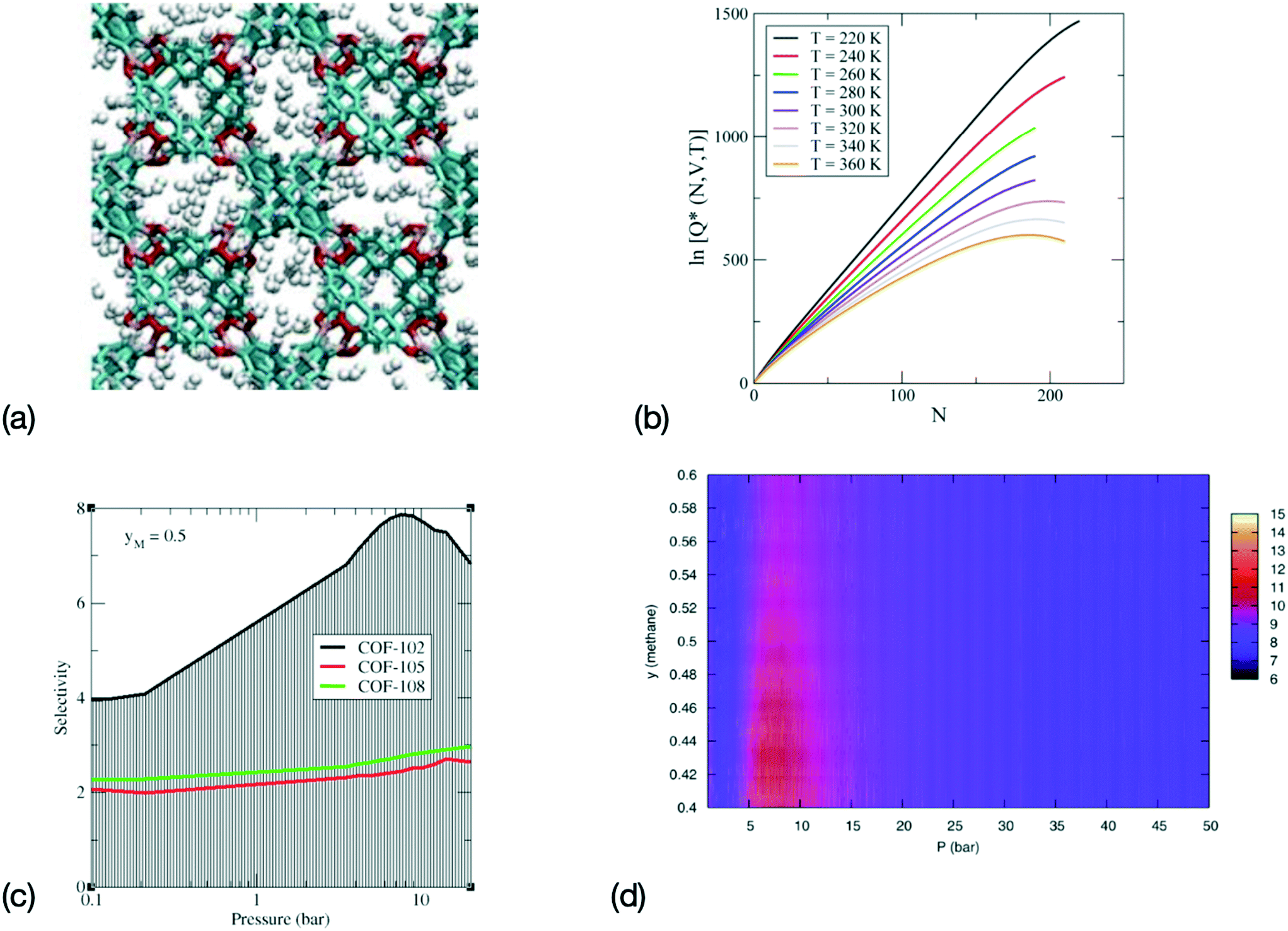 | ||
| Fig. 2 Sequence for a combined MS–ML approach for the determination of the properties of adsorption for gas storage and adsorption in MOFs and COFs. (a) Configurations are generated during MS, for instance here a configuration for a system of H2 adsorbed in COF-108 (adapted with permission from ref. 130, copyright Taylor & Francis), (b) the logarithm of the canonical partition function Q(N, V, T) is computed during MS and trains a ML model. Here representative lnQ(N, V, T) are shown for CO2 in IRMOF-1 (adapted with permission from ref. 129, copyright American Chemical Society), (c) the selectivity can then be derived from the canonical partition function for gas separation in ethane–methane mixtures with a methane mole fraction yM = 0.5 (adapted with permission from ref. 132, copyright American Chemical Society), and (d) immersion free energy for an ethane–methane mixture in COF-102 predicted via the MS-ML approach (adapted with permission from ref. 50, copyright American Chemical Society). | ||
ML has emerged in recent years as an extremely powerful tool to screen a wide range of nanoporous materials for applications in gas storage and separation. Inspired by the development of ML-based materials research,206 the ML-assisted high-throughput computational screening of MOFs and COFs is undergoing tremendous development.202,207 Examples studied through such large-scale screening methods (see Table 1) include the examination of databases of tens of thousands of MOFs for methane and carbon dioxide storage,198 the evaluation of thousands of MOFs membranes for the separation of binary gas mixtures205 and the ML-based selection of MOFs arrays for methane sensing applications.208
| System | Structure database | Notes |
|---|---|---|
| CH4 storage48 | 130938 hMOFs |
Training: 10433 |
| Testing: 119965 |
||
| CH4 storage197 | 137953 hMOFs |
Training: 10000 |
| Testing: 127953 |
||
| CH4 storage198 | 137953 hMOFs |
|
| CO2 storage199 | 324500 hMOFs |
Training: 32450 |
| Testing: 292050 |
||
| CO2 storage200 | 55163 hMOFS |
|
| CO2 storage201 | 400 hMOFs | |
| CO2 storage202 | 100 eMOFs | |
| H2 storage202 | 100 eMOFs | |
| CH4/CO2 separation203 | 324500 hMOFs |
Training: 32450 |
| Testing: 292050 |
||
| CO2/N2 separation204 | 137953 hMOF database |
|
| CO2/CH4 separation205 | 6013 CoRE-MOFMs | Top two structures XUZDUS & XEJXER |
| H2/CH4 separation205 | 6013 CoRE-MOFMs | Top candidates TESGUU & ZIJOF |
| O2/N2 separation205 | 6013 CoRE-MOFMs | Top candidates GETXAG & GOLQII |
| CO2/CH4 separation205 | 6013 CoRE-MOFMs | Top candidates YEKWOC & BAHGUN04 |
5 ML-guided exploration of free energy landscapes
As discussed in previous sections, ML models can be trained on datasets generated by molecular simulations, as a way to interpolate and/or extrapolate the data for conditions that are not covered by the simulations. This leads to ML predictions that have an accuracy close to the simulations for only a fraction of the computational costs, and thus as a way to accelerate the discovery of new materials for a wide range of applications, including high entropy alloys,209 novel glass-forming metallic systems,210 materials with improved catalytic performance,158,159 and complex tasks, such as the prediction of activation energies14,211 or the elucidation of the polymorph selection process.13,212 Operating conditions for a given system can be fine-tuned almost instantly through ML models, which provides another path towards an acceleration of purely MS schemes.Very interestingly, recent work has shown that ML methods can go beyond such interpolation/extrapolation tasks and enable the exploration of high-dimensional free energy landscapes,213 defined by cost functions associated with machine learning. In another example, free energy landscapes, associated with complex assembly processes, can be explored using enhanced sampling simulations for which the reaction coordinate is estimated from a combined MS–ML approach.45 For instance, crystal nucleation has been simulated with umbrella sampling MS along an entropic pathway, i.e. with an entropic reaction coordinate estimated on-the-fly from a machine learned Helmholtz free energy and from the current MS internal energy for each step of the enhanced sampling simulations. This combined approach allows for the exploration of novel pathways spanned by a ML-guided reaction coordinate, and, in turn, can shed light on the pathways underlying a wide range of activated processes and rare events.
In recent years, combined MS–ML approaches156 have been developed using either ANNs, recurrent neural networks,214–217 convolutional neural networks218–222 or autoencoders.223–227 In particular, combinations of deep learning methods with molecular simulations have started to demonstrate great potential in understanding the role played by the collective variables (CVs) that underlie the evolution of a molecular system.228 Such combined approaches can also yield accurate low-dimensional system representations, along which enhanced sampling simulations can be carried out. These methods can be extended to biological systems, as shown in recent work on oligopeptides using different ML strategies such as neural networks, kernel ridge regression, support vector machines and weighted neighbor schemes.139 In particular, the use of autoencoders to learn nonlinear CVs, that are differentiable functions of atomic coordinates, and their use in enhanced sampling simulations can greatly accelerate the exploration of folding free energy landscapes in macromolecular and biological systems.225 New advances in the selection of appropriate CVs for enhanced sampling simulations have also been recently implemented with the use of supervised machine learning.229 Decision functions in supervised machine learning methods can be used as initial CVs for enhanced sampling, and the distance to the support vector machines-decision hyperplane, the output probability estimates from logistic regression or the outputs from neural network classifiers can be leveraged to sample structural changes. Another approach consists in combining both ML and variational inference230 to predict and discover collective variables using deep Bayesian models, with applications to polypeptides231 and to chemical reactions.232
The sampling of rugged free energy landscapes has been the focus of considerable attention in recent years. For instance, adaptive enhanced sampling by force-biasing using neural networks (FUNN) has been shown to perform especially well for systems as diverse as simple particles, proteins and coarse-grained polymer chains.233 In studies of phase transformations, path collective variables can be defined in a space spanned by global classifiers derived from local structural units, identified via a neural-network-based classification scheme.234 Another approach relies on an analogy with reinforcement learning to explore the configurational space, i.e. carrying out a reinforced dynamics for enhanced sampling. This, in turn, allows to capture accurately the structural changes undergone by proteins in explicit solvent models.235 The combination of statistical mechanics with generative learning can also result in the formulation of a competing game between sampling engine and virtual discriminator. This approach has been applied to many-body Hamiltonian systems, with a targeted adversarial learning optimized sampling (TALOS) driving the system to a user-defined target distribution in order to bolster the sampling of rare events.236
Another emerging idea consists in using coarse-grained free energy landscapes, with the aim of reducing the time scales necessary to accurately sample the conformational topology for complex chemical and biological systems. In particular, the back-mapping based sampling method237 back-maps coarse-grained free energy landscapes to create starting points, with a resolution at the atomic level, for molecular simulations. Applications to oligopeptides have demonstrated a gain in efficiency of an order of magnitude for sampling transitions in heptamers, when compared with purely MS approaches. Similarly, coarse-grained methods can also be used for the conformational sampling of proteins and peptide chains, using a neural network to determine free energy surfaces from MS, and then leveraging the machine learned free energy surfaces to carry out simulations with a resolution at the coarse-grained level.26 Nonlinear manifold learning techniques can also be employed to accelerate the exploration of free energy surfaces, by biasing the MD simulator towards unexplored regions using the smoothness of the geometry of the surface.238
ML methods have also become increasingly instrumental in guiding free energy simulations when studying solvation environments162,239 or protein folding.152,156 Such approaches have also been applied to the determination of free energy landscapes for protein–ligand unbinding via metadynamics.240 Metadynamics can also be combined with a Hamiltonian replica-exchange algorithm (sampling water interfaces through scaled Hamiltonians or SWISH) and a machine learned-pathlike variable to compute the binding free energy for a series of chemically diverse ligands with a complex target (human soluble epoxide hydrolase) and to shed light on the role of water in the binding process.241 In recent work, combinations of supervised and unsupervised machine learning techniques have been applied to observables extracted from MS, with the aim of better understanding protein–ligand binding in the context of drug resistance in HIV-1 protease.166 Reinforcement learning adaptive sampling strategies, like the REinforcement learning based Adaptive samPling (REAP) method, provide on-the-fly estimates for the significance of collective variables for the exploration of the folding free energy landscape of proteins, and promotes the exploration of the landscape along key degrees of freedom.242 Another deep learning approach to study ligand–protein systems is the reweighted autoencoded variational Bayes for enhanced sampling (RAVE).243 Recent extensions have allowed learning of reaction coordinate expressed as a linear piecewise function, leading to an efficient protocol for the simulation of slow unbinding processes in practical ligand–protein complexes in an automated manner.
6 Conclusions
Data-driven methods have led to recent advances in the discovery of novel materials. Furthermore, combinations of machine learning with molecular simulation algorithms has provided a way to accelerate conventional computational methods, and as such, have significantly increased the number, the range and the complexity of systems that can be studied and screened as candidates for specific applications. This review first focuses on the determination of free energy via combined ML–MS approaches and examines examples of systems encompassing molecular fluids, biological systems, as well as fluid confined in nanoporous materials known as MOFs and COFs. Free energy simulations are often very computationally intensive and generally require the implementation of enhanced sampling methods for an accurate sampling of high-dimensional free energy surfaces. We thus discuss recent approaches to compute the free energy and how ML models can be trained using simulation data as training datasets. As illustrated by a series of examples presented here, the idea of such combined MS–ML approaches is to predict as accurately and as efficiently as possible the free energy, with the aim e.g. of shedding light on phase transition processes in molecular systems or on conformational changes and folding in biological systems. For nanoconfined systems, the goal is to screen as rapidly as possible materials as candidates for gas storage and gas separation applications. Given the huge number of MOFs and COFs structures that can potentially be synthesized, a purely MS computational screening of all possible structures remains a daunting task. In that case, ML-based screening methods244 can narrow down the field of nanoporous materials that are candidates for a specific application, before MS methods,58,245 or, alternatively, combined MS–ML approaches,246 are employed to test and characterize a smaller set of materials. Combined MS–ML approaches can also considerably accelerate, for instance, the computationally intensive search of the parameter space for the adsorption of multicomponent mixtures, or the determination of the free energy of immersion that quantifies the cost of regenerating the adsorbent for practical applications. The last part of the review examines several new exciting trends in combined MS–ML approaches. Such developments include the ML-guided exploration of free energy landscapes and the ML-aided identification of the crucial parameters and collective variables that underlie the occurrence of rare events in molecular and biological systems and the transitions they undergo between states. These new approaches are especially promising, as they allow for the exploration of as yet unexplored pathways for assembly, chemical reactions or folding processes, and will likely provide new insights in these phenomena.Conflicts of interest
There are no conflicts to declare.Acknowledgements
Partial funding for this research was provided by NSF through award CHE-1955403.References
- J. Behler, J. Chem. Phys., 2016, 145, 170901 CrossRef.
- K. T. Butler, D. W. Davies, H. Cartwright, O. Isayev and A. Walsh, Nature, 2018, 559, 547–555 CrossRef CAS.
- J. Hachmann, M. A. F. Afzal, M. Haghighatlari and Y. Pal, Mol. Simul., 2018, 44, 921–929 CrossRef CAS.
- M. Ceriotti, J. Chem. Phys., 2019, 150, 150901 CrossRef.
- F. Häse, S. Valleau, E. Pyzer-Knapp and A. Aspuru-Guzik, Chem. Sci., 2016, 7, 5139–5147 RSC.
- B. R. Hough, D. A. Beck, D. T. Schwartz and J. Pfaendtner, Comput. Chem. Eng., 2017, 104, 56–63 CrossRef CAS.
- W. Beckner and J. Pfaendtner, J. Chem. Inf. Model., 2019, 59, 2617–2625 CrossRef CAS.
- R. Gómez-Bombarelli, J. N. Wei, D. Duvenaud, J. M. Hernández-Lobato, B. Sánchez-Lengeling, D. Sheberla, J. Aguilera-Iparraguirre, T. D. Hirzel, R. P. Adams and A. Aspuru-Guzik, ACS Cent. Sci., 2018, 4, 268–276 CrossRef.
- D. K. Duvenaud, D. Maclaurin, J. Iparraguirre, R. Bombarell, T. Hirzel, A. Aspuru-Guzik and R. P. Adams, Advances in neural information processing systems, 2015, pp. 2224–2232 Search PubMed.
- B. Sanchez-Lengeling and A. Aspuru-Guzik, Science, 2018, 361, 360–365 CrossRef CAS.
- T. Barnard, H. Hagan, S. Tseng and G. C. Sosso, Mol. Syst. Des. Eng., 2020, 5, 317–329 RSC.
- J. P. Janet, L. Chan and H. J. Kulik, J. Phys. Chem. Lett., 2018, 9, 1064–1071 CrossRef CAS.
- F. Musil, S. De, J. Yang, J. E. Campbell, G. M. Day and M. Ceriotti, Chem. Sci., 2018, 9, 1289–1300 RSC.
- C. A. Grambow, L. Pattanaik and W. H. Green, J. Phys. Chem. Lett., 2020, 11, 2992–2997 CrossRef CAS.
- G. M. Rotskoff and E. Vanden-Eijnden, Stat, 2018, 1050, 22 Search PubMed.
- G. Carleo, I. Cirac, K. Cranmer, L. Daudet, M. Schuld, N. Tishby, L. Vogt-Maranto and L. Zdeborová, Rev. Mod. Phys., 2019, 91, 045002 CrossRef CAS.
- C. M. Handley and P. L. Popelier, J. Phys. Chem. A, 2010, 114, 3371–3383 CrossRef CAS.
- J. Behler, Phys. Chem. Chem. Phys., 2011, 13, 17930–17955 RSC.
- J. Behler, J. Phys.: Condens. Matter, 2014, 26, 183001 CrossRef CAS.
- B. Jiang, J. Li and H. Guo, Int. Rev. Phys. Chem., 2016, 35, 479–506 Search PubMed.
- J. S. Smith, O. Isayev and A. E. Roitberg, Chem. Sci., 2017, 8, 3192–3203 RSC.
- F. Nüske, L. Boninsegna and C. Clementi, J. Chem. Phys., 2019, 151, 044116 CrossRef.
- G. C. Sosso, V. L. Deringer, S. R. Elliott and G. Csányi, Mol. Simul., 2018, 44, 866–880 CrossRef CAS.
- R. Barrett, M. Chakraborty, D. B. Amirkulova, H. A. Gandhi, G. P. Wellawatte and A. D. White, J. Open Source Softw., 2020, 5, 2367 CrossRef.
- Z. Li, G. P. Wellawatte, M. Chakraborty, H. A. Gandhi, C. Xu and A. D. White, Chem. Sci., 2020, 11, 9524–9531 RSC.
- T. Lemke and C. Peter, J. Chem. Theory Comput., 2017, 13, 6213–6221 CrossRef CAS.
- F. Häse, I. F. Galván, A. Aspuru-Guzik, R. Lindh and M. Vacher, Chem. Sci., 2019, 10, 2298–2307 RSC.
- C. S. Adorf, J. Antonaglia, J. Dshemuchadse and S. C. Glotzer, J. Chem. Phys., 2018, 149, 204102 CrossRef.
- J. G. Freeze, H. R. Kelly and V. S. Batista, Chem. Rev., 2019, 119, 6595–6612 CrossRef CAS.
- Z. M. Sherman, M. P. Howard, B. A. Lindquist, R. B. Jadrich and T. M. Truskett, J. Chem. Phys., 2020, 152, 140902 CrossRef CAS.
- J. Chen, X. Xu, X. Xu and D. H. Zhang, J. Chem. Phys., 2013, 138, 221104 CrossRef.
- A. J. Ballard, R. Das, S. Martiniani, D. Mehta, L. Sagun, J. D. Stevenson and D. J. Wales, Phys. Chem. Chem. Phys., 2017, 19, 12585–12603 RSC.
- H. E. Sauceda, S. Chmiela, I. Poltavsky, K.-R. Müller and A. Tkatchenko, J. Chem. Phys., 2019, 150, 114102 CrossRef.
- M. Haghighatlari and J. Hachmann, Curr. Opin. Chem. Eng., 2019, 23, 51–57 CrossRef.
- F. Brockherde, L. Vogt, L. Li, M. E. Tuckerman, K. Burke and K.-R. Müller, Nat. Commun., 2017, 8, 1–10 CrossRef CAS.
- J. Wang, S. Olsson, C. Wehmeyer, A. Pérez, N. E. Charron, G. De Fabritiis, F. Noé and C. Clementi, ACS Cent. Sci., 2019, 5, 755–767 CAS.
- C. Duan, J. P. Janet, F. Liu, A. Nandy and H. J. Kulik, J. Chem. Theory Comput., 2019, 15, 2331–2345 CrossRef CAS.
- A. W. Long, J. Zhang, S. Granick and A. L. Ferguson, Soft Matter, 2015, 11, 8141–8153 RSC.
- C. S. Adorf, T. C. Moore, Y. J. Melle and S. C. Glotzer, J. Phys. Chem. B, 2019, 124, 69–78 CrossRef.
- N. E. Jackson, M. A. Webb and J. J. de Pablo, Curr. Opin. Chem. Eng., 2019, 23, 106–114 CrossRef.
- B. Jiang, M. Yang, D. Xie and H. Guo, Chem. Soc. Rev., 2016, 45, 3621–3640 RSC.
- R. A. Mansbach and A. L. Ferguson, J. Chem. Phys., 2015, 142, 03B607_1 CrossRef.
- L. Mones, N. Bernstein and G. Csányi, J. Chem. Theory Comput., 2016, 12, 5100–5110 CrossRef CAS.
- E. Schneider, L. Dai, R. Q. Topper, C. Drechsel-Grau and M. E. Tuckerman, Phys. Rev. Lett., 2017, 119, 150601 CrossRef.
- C. Desgranges and J. Delhommelle, Phys. Rev. E, 2018, 98, 063307 CrossRef CAS.
- F. Noé, S. Olsson, J. Köhler and H. Wu, Science, 2019, 365, eaaw1147 CrossRef.
- M. O. Jäger, E. V. Morooka, F. F. Canova, L. Himanen and A. S. Foster, npj Comput. Mater., 2018, 4, 1–8 CrossRef.
- M. Pardakhti, E. Moharreri, D. Wanik, S. L. Suib and R. Srivastava, ACS Comb. Sci., 2017, 19, 640–645 CrossRef CAS.
- A. Ahmed, S. Seth, J. Purewal, A. G. Wong-Foy, M. Veenstra, A. J. Matzger and D. J. Siegel, Nat. Commun., 2019, 10, 1–9 CrossRef CAS.
- C. Desgranges and J. Delhommelle, J. Phys. Chem. C, 2019, 124, 1907–1917 CrossRef.
- G. Anderson, B. Schweitzer, R. Anderson and D. A. Gomez-Gualdron, J. Phys. Chem. C, 2018, 123, 120–130 CrossRef.
- X. Wu, S. Xiang, J. Su and W. Cai, J. Phys. Chem. C, 2019, 123, 8550–8559 CrossRef CAS.
- N. S. Bobbitt and R. Q. Snurr, Mol. Simul., 2019, 45, 1069–1081 CrossRef CAS.
- R. Anderson, A. Biong and D. A. Gómez-Gualdrón, J. Chem. Theory Comput., 2020, 16, 1271–1283 CrossRef CAS.
- G. Bussi and A. Laio, Nat. Rev. Phys., 2020, 1–13 Search PubMed.
- T. Toyao, K. Suzuki, S. Kikuchi, S. Takakusagi, K.-i. Shimizu and I. Takigawa, J. Phys. Chem. C, 2018, 122, 8315–8326 CrossRef CAS.
- Z. Zhang, J. A. Schott, M. Liu, H. Chen, X. Lu, B. G. Sumpter, J. Fu and S. Dai, Angew. Chem., 2019, 131, 265–269 CrossRef.
- K. M. Jablonka, D. Ongari, S. M. Moosavi and B. Smit, Chem. Rev., 2020, 120, 8066–8129 CrossRef CAS.
- M. B. Christopher, Pattern Recognition and Machine Learning, Springer-Verlag, New York, 2016 Search PubMed.
- K. Hansen, G. Montavon, F. Biegler, S. Fazli, M. Rupp, M. Scheffler, O. A. Von Lilienfeld, A. Tkatchenko and K.-R. Müller, J. Chem. Theory Comput., 2013, 9, 3404–3419 CrossRef CAS.
- P. O. Dral, O. A. von Lilienfeld and W. Thiel, J. Chem. Theory Comput., 2015, 11, 2120–2125 CrossRef CAS.
- M. Rupp, A. Tkatchenko, K.-R. Müller and O. A. Von Lilienfeld, Phys. Rev. Lett., 2012, 108, 058301 CrossRef.
- J. B. Witkoskie and D. J. Doren, J. Chem. Theory Comput., 2005, 1, 14–23 CrossRef CAS.
- T. Straatsma and J. McCammon, J. Chem. Phys., 1991, 95, 1175–1188 CrossRef CAS.
- J. Kästner and W. Thiel, J. Chem. Phys., 2005, 123, 144104 CrossRef.
- M. R. Shirts and V. S. Pande, J. Chem. Phys., 2005, 122, 144107 CrossRef.
- M. Müller and K. C. Daoulas, J. Chem. Phys., 2008, 128, 024903 CrossRef.
- D. A. Kofke, Fluid Phase Equilib., 2005, 228, 41–48 CrossRef.
- D. Frenkel and A. J. Ladd, J. Chem. Phys., 1984, 81, 3188–3193 CrossRef CAS.
- E. J. Meijer, D. Frenkel, R. A. LeSar and A. J. Ladd, J. Chem. Phys., 1990, 92, 7570–7575 CrossRef CAS.
- G. M. Torrie and J. P. Valleau, J. Comput. Phys., 1977, 23, 187–199 CrossRef.
- C. Bartels and M. Karplus, J. Comput. Chem., 1997, 18, 1450–1462 CrossRef CAS.
- P. Virnau and M. Müller, J. Chem. Phys., 2004, 120, 10925–10930 CrossRef CAS.
- G. Bussi, A. Laio and M. Parrinello, Phys. Rev. Lett., 2006, 96, 090601 CrossRef.
- A. Barducci, G. Bussi and M. Parrinello, Phys. Rev. Lett., 2008, 100, 020603 CrossRef.
- J. F. Dama, M. Parrinello and G. A. Voth, Phys. Rev. Lett., 2014, 112, 240602 CrossRef.
- A. Laio and F. L. Gervasio, Rep. Prog. Phys., 2008, 71, 126601 CrossRef.
- J. Kästner, Wiley Interdiscip. Rev.: Comput. Mol. Sci., 2011, 1, 932–942 Search PubMed.
- P. R. Ten Wolde, M. J. Ruiz-Montero and D. Frenkel, Phys. Rev. Lett., 1995, 75, 2714 CrossRef CAS.
- P. Rein ten Wolde, M. J. Ruiz-Montero and D. Frenkel, J. Chem. Phys., 1996, 104, 9932–9947 CrossRef.
- S. Auer and D. Frenkel, Nature, 2001, 409, 1020–1023 CrossRef CAS.
- A. Cacciuto, S. Auer and D. Frenkel, Nature, 2004, 428, 404–406 CrossRef CAS.
- C. Desgranges and J. Delhommelle, Phys. Rev. Lett., 2007, 98, 235502 CrossRef.
- C. Desgranges and J. Delhommelle, J. Am. Chem. Soc., 2011, 133, 2872–2874 CrossRef CAS.
- R. Ni and M. Dijkstra, J. Chem. Phys., 2011, 134, 034501 CrossRef.
- M. Gonzalez, E. Sanz, C. McBride, J. Abascal, C. Vega and C. Valeriani, Phys. Chem. Chem. Phys., 2014, 16, 24913–24919 RSC.
- C. Desgranges and J. Delhommelle, J. Am. Chem. Soc., 2014, 136, 8145–8148 CrossRef CAS.
- C. Desgranges and J. Delhommelle, Phys. Rev. Lett., 2018, 120, 115701 CrossRef CAS.
- B. Chen, J. I. Siepmann, K. J. Oh and M. L. Klein, J. Chem. Phys., 2001, 115, 10903–10913 CrossRef CAS.
- H. Wang, H. Gould and W. Klein, Phys. Rev. E, 2007, 76, 031604 CrossRef.
- C. Desgranges and J. Delhommelle, J. Chem. Phys., 2016, 145, 204112 CrossRef.
- C. Desgranges and J. Delhommelle, J. Chem. Phys., 2016, 145, 234505 CrossRef.
- C. Desgranges and J. Delhommelle, J. Chem. Phys., 2017, 146, 184104 CrossRef.
- C. Desgranges and J. Delhommelle, Langmuir, 2019, 35, 15401–15409 CrossRef CAS.
- C. Desgranges and J. Delhommelle, J. Phys. Chem. C, 2019, 123, 11707–11713 CrossRef CAS.
- L. Filion, M. Hermes, R. Ni and M. Dijkstra, J. Chem. Phys., 2010, 133, 244115 CrossRef CAS.
- C. Desgranges and J. Delhommelle, Phys. Rev. Lett., 2019, 123, 195701 CrossRef CAS.
- C. Dellago, P. Bolhuis and P. L. Geissler, Adv. Chem. Phys., 2002, 123, 1–78 CAS.
- C. Dellago and P. G. Bolhuis, in Advanced Computer Simulation Approaches for Soft Matter Sciences III, Springer, 2009, pp. 167–233 Search PubMed.
- T. S. Van Erp and P. G. Bolhuis, J. Comput. Phys., 2005, 205, 157–181 CrossRef.
- E. E. Borrero, M. Weinwurm and C. Dellago, J. Chem. Phys., 2011, 134, 244118 CrossRef.
- L. Rosso, J. B. Abrams and M. E. Tuckerman, J. Phys. Chem. B, 2005, 109, 4162–4167 CrossRef CAS.
- M. A. Cuendet and M. E. Tuckerman, J. Chem. Theory Comput., 2014, 10, 2975–2986 CrossRef CAS.
- C. Jarzynski, Phys. Rev. Lett., 1997, 78, 2690 CrossRef CAS.
- G. E. Crooks, Phys. Rev. E, 1999, 60, 2721 CrossRef CAS.
- D. J. Evans, Mol. Phys., 2003, 101, 1551–1554 CrossRef CAS.
- M. S. Shell, P. G. Debenedetti and A. Z. Panagiotopoulos, Phys. Rev. E, 2002, 66, 056703 CrossRef.
- J. R. Errington, J. Chem. Phys., 2003, 118, 9915–9925 CrossRef CAS.
- G. Gazenmüller and P. J. Camp, J. Chem. Phys., 2007, 127, 154504 CrossRef.
- C. Desgranges and J. Delhommelle, J. Chem. Phys., 2009, 130, 244109 CrossRef.
- T. Aleksandrov, C. Desgranges and J. Delhommelle, Fluid Phase Equilib., 2010, 287, 79–83 CrossRef CAS.
- C. Desgranges and J. Delhommelle, J. Chem. Phys., 2012, 136, 184107 CrossRef.
- K. S. Rane, S. Murali and J. R. Errington, J. Chem. Theory Comput., 2013, 9, 2552–2566 CrossRef CAS.
- F. Wang and D. P. Landau, Phys. Rev. E, 2001, 64, 056101 CrossRef CAS.
- F. Wang and D. Landau, Phys. Rev. Lett., 2001, 86, 2050–2053 CrossRef CAS.
- Q. Yan, R. Faller and J. J. de Pablo, J. Chem. Phys., 2002, 116, 8745–8750 CrossRef CAS.
- C. Desgranges and J. Delhommelle, Energy Fuels, 2017, 31, 10699–10705 CrossRef CAS.
- K. N. Ngale, C. Desgranges and J. Delhommelle, Mol. Simul., 2012, 38, 653–658 CrossRef CAS.
- T. Aleksandrov, C. Desgranges and J. Delhommelle, Mol. Simul., 2012, 38, 1265–1270 CrossRef CAS.
- C. Desgranges and J. Delhommelle, J. Chem. Phys., 2018, 149, 072307 CrossRef.
- C. Desgranges and J. Delhommelle, J. Chem. Phys., 2012, 136, 184108 CrossRef.
- C. Desgranges and J. Delhommelle, J. Chem. Phys., 2014, 140, 104109 CrossRef.
- C. Desgranges and J. Delhommelle, J. Chem. Phys., 2016, 144, 124510 CrossRef.
- C. Desgranges and J. Delhommelle, J. Chem. Phys., 2016, 145, 184504 CrossRef.
- C. Desgranges and J. Delhommelle, J. Chem. Theory Comput., 2015, 11, 5401 CrossRef CAS.
- C. Desgranges, A. Margo and J. Delhommelle, Chem. Phys. Lett., 2016, 658, 37–42 CrossRef CAS.
- C. Desgranges and J. Delhommelle, J. Chem. Eng. Data, 2017, 62, 4032–4040 CrossRef CAS.
- C. Desgranges and J. Delhommelle, J. Phys. Chem. B, 2014, 118, 3175 CrossRef CAS.
- J. M. Hicks, C. Desgranges and J. Delhommelle, J. Phys. Chem. C, 2012, 116, 22938–22946 CrossRef CAS.
- A. R. V. Koenig, C. Desgranges and J. Delhommelle, Mol. Simul., 2014, 40, 71–79 CrossRef CAS.
- E. A. Hicks, C. Desgranges and J. Delhommelle, Mol. Simul., 2014, 40, 656–663 CrossRef CAS.
- K. Gopalsamy, C. Desgranges and J. Delhommelle, J. Phys. Chem. C, 2017, 121, 24692–24700 CrossRef CAS.
- V. K. Shen and D. W. Siderius, J. Chem. Phys., 2014, 140, 244106 CrossRef.
- M. Witman, N. A. Mahynski and B. Smit, J. Chem. Theory Comput., 2018, 14, 6149–6158 CrossRef CAS.
- N. A. Mahynski, H. W. Hatch, M. Witman, D. A. Sheen, J. R. Errington and V. K. Shen, Mol. Simul., 2020, 1–13 CrossRef.
- Y. LeCun, L. Bottou, G. B. Orr and K.-R. Müller, Efficient backprop, Springer, 1998, pp. 9–50 Search PubMed.
- C. Desgranges and J. Delhommelle, J. Chem. Phys., 2018, 149, 044118 CrossRef.
- C. Desgranges and J. Delhommelle, Chem. Phys. Lett., 2019, 715, 1–6 CrossRef CAS.
- J. R. Cendagorta, J. Tolpin, E. Schneider, R. Q. Topper and M. E. Tuckerman, J. Phys. Chem. B, 2020, 124, 3647–3660 CrossRef CAS.
- T. G. Dietterich, Multiple Classifier Systems, MCS 2000, 2000, pp. 1–15 Search PubMed.
- A. Krogh and J. Vedelsby, Adv. Neural Inf. Process Syst., 1995, 231–238 Search PubMed.
- L. Breiman, Mach. Learn., 1996, 24, 123–140 Search PubMed.
- I. Goodfellow, Y. Bengio and A. Courville, Deep Learning, MIT press, 2016 Search PubMed.
- A. L. Ferguson, J. Comput. Chem., 2017, 38, 1583–1605 CrossRef CAS.
- N. Chopin, T. Lelièvre and G. Stoltz, Stat. Comput., 2012, 22, 897–916 CrossRef.
- M. Habeck, Phys. Rev. Lett., 2012, 109, 100601 CrossRef.
- G. Hummer, New J. Phys., 2005, 7, 34 CrossRef.
- H. Sidky and J. K. Whitmer, J. Chem. Phys., 2018, 148, 104111 CrossRef.
- L. Maragliano and E. Vanden-Eijnden, J. Chem. Phys., 2008, 128, 184110 CrossRef.
- L. Cao, G. Stoltz, T. Lelièvre, M.-C. Marinica and M. Athènes, J. Chem. Phys., 2014, 140, 03B610_1 Search PubMed.
- T. Stecher, N. Bernstein and G. Csányi, J. Chem. Theory Comput., 2014, 10, 4079–4097 CrossRef CAS.
- S. Mittal and D. Shukla, Mol. Simul., 2018, 44, 891–904 CrossRef CAS.
- M. Karplus, Angew. Chem., Int. Ed., 2014, 53, 9992–10005 CrossRef CAS.
- H. M. Senn and W. Thiel, Angew. Chem., Int. Ed., 2009, 48, 1198–1229 CrossRef CAS.
- H. Lin and D. G. Truhlar, Theor. Chem. Acc., 2007, 117, 185 Search PubMed.
- F. Noé, G. De Fabritiis and C. Clementi, Curr. Opin. Struct. Biol., 2020, 60, 77–84 CrossRef.
- A. Tkatchenko, Nat. Commun., 2020, 11, 1–4 Search PubMed.
- W. Yang, T. T. Fidelis and W.-H. Sun, ACS Omega, 2019, 5, 83–88 CrossRef.
- A. R. Singh, B. A. Rohr, J. A. Gauthier and J. K. Nørskov, Catal. Lett., 2019, 149, 2347–2354 CrossRef CAS.
- C. Chen, W. Ye, Y. Zuo, C. Zheng and S. P. Ong, Chem. Mater., 2019, 31, 3564–3572 CrossRef CAS.
- Y. Wang, J. M. L. Ribeiro and P. Tiwary, Curr. Opin. Struct. Biol., 2020, 61, 139–145 CrossRef CAS.
- Y. Basdogan, M. C. Groenenboom, E. Henderson, S. De, S. B. Rempe and J. A. Keith, J. Chem. Theory Comput., 2019, 16, 633–642 CrossRef.
- J. Scheen, W. Wu, A. S. J. S. Mey, P. Tosco, M. Mackey and J. Michel, ChemRXiv, 2020, DOI:10.26434/chemrxiv.12380612.v1.
- D. Kilburg and E. Gallicchio, J. Chem. Theory Comput., 2018, 14, 6183–6196 CrossRef CAS.
- G. Bitencourt-Ferreira and W. F. de Azevedo, Biophys. Chem., 2018, 240, 63–69 CrossRef CAS.
- T. W. Whitfield, D. A. Ragland, K. B. Zeldovich and C. A. Schiffer, J. Chem. Theory Comput., 2019, 16, 1284–1299 CrossRef.
- D. A. Rufa, H. E. Bruce Macdonald, J. Fass, M. Wieder, P. B. Grinaway, A. E. Roitberg, O. Isayev and J. D. Chodera, bioRxiv, 2020, DOI:10.1101/2020.07.29.227959.
- B. Selvam, S. Mittal and D. Shukla, ACS Cent. Sci., 2018, 4, 1146–1154 CrossRef CAS.
- S. Nayak, S. Bhattacharjee, J.-H. Choi and S. C. Lee, J. Phys. Chem. A, 2019, 124, 247–254 CrossRef.
- T. Toyao, Z. Maeno, S. Takakusagi, T. Kamachi, I. Takigawa and K.-I. Shimizu, ACS Catal., 2019, 10, 2260–2297 CrossRef.
- G. Panapitiya, G. Avendaño-Franco, P. Ren, X. Wen, Y. Li and J. P. Lewis, J. Am. Chem. Soc., 2018, 140, 17508–17514 CrossRef CAS.
- M. Zafari, D. Kumar, M. Umer and K. S. Kim, J. Mater. Chem. A, 2020, 8, 5209–5216 RSC.
- Z. Li, S. Wang, W. S. Chin, L. E. Achenie and H. Xin, J. Mater. Chem. A, 2017, 5, 24131–24138 RSC.
- A. J. Chowdhury, W. Yang, K. E. Abdelfatah, M. Zare, A. Heyden and G. A. Terejanu, J. Chem. Theory Comput., 2020, 16, 1105–1114 CrossRef CAS.
- Z. W. Ulissi, A. J. Medford, T. Bligaard and J. K. Nørskov, Nat. Commun., 2017, 8, 1–7 CrossRef.
- R. Gasper, H. Shi and A. Ramasubramaniam, J. Phys. Chem. C, 2017, 121, 5612–5619 CrossRef CAS.
- R. A. Hoyt, M. M. Montemore, I. Fampiou, W. Chen, G. Tritsaris and E. Kaxiras, J. Chem. Inf. Model., 2019, 59, 1357–1365 CrossRef CAS.
- K. Takahashi and I. Miyazato, J. Comput. Chem., 2018, 39, 2405–2408 CrossRef CAS.
- Z. W. Ulissi, A. R. Singh, C. Tsai and J. K. Nørskov, J. Phys. Chem. Lett., 2016, 7, 3931–3935 CrossRef CAS.
- S. Chong, S. Lee, B. Kim and J. Kim, Coord. Chem. Rev., 2020, 423, 213487 CrossRef CAS.
- G. S. Fanourgakis, K. Gkagkas, E. Tylianakis, E. Klontzas and G. Froudakis, J. Phys. Chem. A, 2019, 123, 6080–6087 CrossRef CAS.
- H. Dureckova, M. Krykunov, M. Z. Aghaji and T. K. Woo, J. Phys. Chem. C, 2019, 123, 4133–4139 CrossRef CAS.
- H. Sui, L. Li, X. Zhu, D. Chen and G. Wu, Chemosphere, 2016, 144, 1950–1959 CrossRef CAS.
- N. L. Rosi, J. Eckert, M. Eddaoudi, D. T. Vodak, J. Kim, M. O'Keeffe and O. M. Yaghi, Science, 2003, 300, 1127–1129 CrossRef CAS.
- J. L. Rowsell, A. R. Millward, K. S. Park and O. M. Yaghi, J. Am. Chem. Soc., 2004, 126, 5666–5667 CrossRef CAS.
- D. Sun, S. Ma, Y. Ke, D. J. Collins and H.-C. Zhou, J. Am. Chem. Soc., 2006, 128, 3896–3897 CrossRef CAS.
- H. Furukawa, M. A. Miller and O. M. Yaghi, J. Mater. Chem., 2007, 17, 3197–3204 RSC.
- S. S. Han, H. Furukawa, O. M. Yaghi and W. A. Goddard Iii, J. Am. Chem. Soc., 2008, 130, 11580–11581 CrossRef CAS.
- A. Gopalan, B. J. Bucior, N. S. Bobbitt and R. Q. Snurr, Mol. Phys., 2019, 117, 3683–3694 CrossRef CAS.
- S.-Y. Kim, S.-I. Kim and Y.-S. Bae, J. Phys. Chem. C, 2020, 124, 19538–19547 CrossRef CAS.
- G. S. Fanourgakis, K. Gkagkas, E. Tylianakis and G. Froudakis, J. Phys. Chem. C, 2020, 124, 7117–7126 CrossRef CAS.
- K. S. Deeg, D. Damasceno Borges, D. Ongari, N. Rampal, L. Talirz, A. V. Yakutovich, J. M. Huck and B. Smit, ACS Appl. Mater. Interfaces, 2020, 12, 21559–21568 CrossRef CAS.
- Y. Sun, R. F. DeJaco and J. I. Siepmann, Chem. Sci., 2019, 10, 4377–4388 RSC.
- C. E. Wilmer, M. Leaf, C. Y. Lee, O. K. Farha, B. G. Hauser, J. T. Hupp and R. Q. Snurr, Nat. Chem., 2012, 4, 83 CrossRef CAS.
- F. H. Allen, Acta Crystallogr., Sect. B: Struct. Sci., 2002, 58, 380–388 CrossRef.
- Y. G. Chung, J. Camp, M. Haranczyk, B. J. Sikora, W. Bury, V. Krungleviciute, T. Yildirim, O. K. Farha, D. S. Sholl and R. Q. Snurr, Chem. Mater., 2014, 26, 6185–6192 CrossRef CAS.
- M. Fernandez, T. K. Woo, C. E. Wilmer and R. Q. Snurr, J. Phys. Chem. C, 2013, 117, 7681–7689 CrossRef CAS.
- G. S. Fanourgakis, K. Gkagkas, E. Tylianakis and G. E. Froudakis, J. Am. Chem. Soc., 2020, 142, 3814–3822 CrossRef CAS.
- M. Fernandez, P. G. Boyd, T. D. Daff, M. Z. Aghaji and T. K. Woo, J. Phys. Chem. Lett., 2014, 5, 3056–3060 CrossRef CAS.
- Y. G. Chung, E. Haldoupis, B. J. Bucior, M. Haranczyk, S. Lee, H. Zhang, K. D. Vogiatzis, M. Milisavljevic, S. Ling and J. S. Camp, et al. , J. Chem. Eng. Data, 2019, 64, 5985–5998 CrossRef CAS.
- R. Anderson, J. Rodgers, E. Argueta, A. Biong and D. A. Gómez-Gualdrón, Chem. Mater., 2018, 30, 6325–6337 CrossRef CAS.
- G. Borboudakis, T. Stergiannakos, M. Frysali, E. Klontzas, I. Tsamardinos and G. E. Froudakis, npj Comput. Mater., 2017, 3, 1–7 CrossRef CAS.
- M. Z. Aghaji, M. Fernandez, P. G. Boyd, T. D. Daff and T. K. Woo, Eur. J. Inorg. Chem., 2016, 2016, 4505–4511 CrossRef CAS.
- M. Fernandez and A. S. Barnard, ACS Comb. Sci., 2016, 18, 243–252 CrossRef CAS.
- W. Yang, H. Liang, F. Peng, Z. Liu, J. Liu and Z. Qiao, Nanomaterials, 2019, 9, 467 CrossRef CAS.
- T. Zhou, Z. Song and K. Sundmacher, Engineering, 2019, 5, 1017–1026 CrossRef CAS.
- Z. Shi, W. Yang, X. Deng, C. Cai, Y. Yan, H. Liang, Z. Liu and Z. Qiao, Mol. Syst. Des. Eng., 2020, 5, 725–742 RSC.
- J. A. Gustafson and C. E. Wilmer, ACS Sens., 2019, 4, 1586–1593 CrossRef CAS.
- Z. Zhou, Y. Zhou, Q. He, Z. Ding, F. Li and Y. Yang, npj Comput. Mater., 2019, 5, 1–9 CrossRef.
- F. Ren, L. Ward, T. Williams, K. J. Laws, C. Wolverton, J. Hattrick-Simpers and A. Mehta, Sci. Adv., 2018, 4, eaaq1566 CrossRef.
- O. A. von Lilienfeld, K.-R. Müller and A. Tkatchenko, Nat. Rev. Chem., 2020, 1–12 Search PubMed.
- J. Yang, N. Li and S. Li, CrystEngComm, 2019, 21, 6173–6185 RSC.
- D. J. Wales, Annu. Rev. Physiol., 2018, 69, 401–425 CrossRef CAS.
- J. Kadupitiya, G. C. Fox and V. Jadhao, ArXiv e-prints, 2020, arXiv:2004.06493 Search PubMed.
- L. Simine, T. C. Allen and P. J. Rossky, Proc. Natl. Acad. Sci. U. S. A., 2020, 117, 13945–13948 CrossRef CAS.
- J. Wang, C. Li, S. Shin and H. Qi, J. Phys. Chem. C, 2020, 124, 14838–14846 CrossRef CAS.
- E. Pfeiffenberger and P. A. Bates, PLoS One, 2018, 13, e0202652 CrossRef.
- T. Fukuya and Y. Shibuta, Comput. Mater. Sci., 2020, 184, 109880 CrossRef CAS.
- J. Li, W. Zhu, J. Wang, W. Li, S. Gong, J. Zhang and W. Wang, PLoS Comput. Biol., 2018, 14, e1006514 CrossRef.
- J. Jiménez, M. Skalic, G. Martinez-Rosell and G. De Fabritiis, J. Chem. Inf. Model., 2018, 58, 287–296 CrossRef.
- K. Ryczko, K. Mills, I. Luchak, C. Homenick and I. Tamblyn, Comput. Mater. Sci., 2018, 149, 134–142 CrossRef CAS.
- K. Schütt, P.-J. Kindermans, H. E. S. Felix, S. Chmiela, A. Tkatchenko and K.-R. Müller, Adv. Neural Inf. Process Syst., 2017, 991–1001 Search PubMed.
- W. Wang and R. Gómez-Bombarelli, npj Comput. Mater., 2019, 5, 1–9 CrossRef.
- P. Rajak, A. Krishnamoorthy, A. Nakano, P. Vashishta and R. Kalia, Phys. Rev. B, 2019, 100, 014108 CrossRef CAS.
- W. Chen and A. L. Ferguson, J. Comput. Chem., 2018, 39, 2079–2102 CrossRef CAS.
- C. Wehmeyer and F. Noé, J. Chem. Phys., 2018, 148, 241703 CrossRef.
- A. Moradzadeh and N. R. Aluru, J. Phys. Chem. Lett., 2019, 10, 7568–7576 CrossRef CAS.
- H. Sidky, W. Chen and A. L. Ferguson, Mol. Phys., 2020, 118, e1737742 CrossRef.
- M. M. Sultan and V. S. Pande, J. Chem. Phys., 2018, 149, 094106 CrossRef.
- L. Bonati, Y.-Y. Zhang and M. Parrinello, Proc. Natl. Acad. Sci. U. S. A., 2019, 116, 17641–17647 CrossRef CAS.
- M. Schöberl, N. Zabaras and P.-S. Koutsourelakis, J. Chem. Phys., 2019, 150, 024109 CrossRef.
- L. Bonati, V. Rizzi and M. Parrinello, J. Phys. Chem. Lett., 2020, 11, 2998–3004 CrossRef CAS.
- A. Z. Guo, E. Sevgen, H. Sidky, J. K. Whitmer, J. A. Hubbell and J. J. de Pablo, J. Chem. Phys., 2018, 148, 134108 CrossRef.
- J. Rogal, E. Schneider and M. E. Tuckerman, Phys. Rev. Lett., 2019, 123, 245701 CrossRef CAS.
- L. Zhang, H. Wang and E. Weinan, J. Chem. Phys., 2018, 148, 124113 CrossRef.
- J. Zhang, Y. I. Yang and F. Noé, J. Phys. Chem. Lett., 2019, 10, 5791–5797 CrossRef CAS.
- S. Hunkler, T. Lemke, C. Peter and O. Kukharenko, J. Chem. Phys., 2019, 151, 154102 CrossRef.
- E. Chiavazzo, R. Covino, R. R. Coifman, C. W. Gear, A. S. Georgiou, G. Hummer and I. G. Kevrekidis, Proc. Natl. Acad. Sci. U. S. A., 2017, 114, E5494–E5503 CrossRef CAS.
- P. Zhang, L. Shen and W. Yang, J. Phys. Chem. B, 2018, 123, 901–908 CrossRef.
- R. Capelli, A. Bochicchio, G. Piccini, R. Casasnovas, P. Carloni and M. Parrinello, J. Chem. Theory Comput., 2019, 15, 3354–3361 CrossRef CAS.
- R. Evans, L. Hovan, G. A. Tribello, B. P. Cossins, C. Estarellas and F. L. Gervasio, J. Chem. Theory Comput., 2020, 16, 4641–4654 CrossRef CAS.
- Z. Shamsi, K. J. Cheng and D. Shukla, J. Phys. Chem. B, 2018, 122, 8386–8395 CrossRef CAS.
- J. M. Lamim Ribeiro and P. Tiwary, J. Chem. Theory Comput., 2018, 15, 708–719 CrossRef.
- I. Tsamardinos, G. S. Fanourgakis, E. Greasidou, E. Klontzas, K. Gkagkas and G. E. Froudakis, Microporous Mesoporous Mater., 2020, 110160 CrossRef CAS.
- D. Ongari, L. Talirz and B. Smit, ACS Cent. Sci., 2020, 6, 1890–1900 CrossRef CAS.
- X. Zhang, K. Zhang and Y. Lee, ACS Appl. Mater. Interfaces, 2019, 12, 734–743 CrossRef.
| This journal is © The Royal Society of Chemistry 2021 |