
 Open Access Article
 This Open Access Article is licensed under a Creative Commons Attribution-Non Commercial 3.0 Unported Licence
A reaction-coordinate perspective of magnetic relaxation
Cassidy E.
Jackson
,
Ian P.
Moseley
 ,
Roxanna
Martinez
,
Siyoung
Sung
and
Joseph M.
Zadrozny
*
,
Roxanna
Martinez
,
Siyoung
Sung
and
Joseph M.
Zadrozny
*
Department of Chemistry, Colorado State University, Fort Collins, CO, USA. E-mail: joe.zadrozny@colostate.edu
First published on 4th May 2021
Abstract
Understanding and utilizing the dynamic quantum properties of metal ions is the frontier of many next generation technologies. One property in particular, magnetic relaxation, is a complicated physical phenomenon that is scarcely treated in undergraduate coursework. Consequently, principles of magnetic relaxation are nearly impenetrable to starting synthetic chemists, who ultimately design the molecules that fuel new discoveries. In this Tutorial Review, we describe a new paradigm for thinking of magnetic relaxation in metal complexes in terms of a simple reaction-coordinate diagram to facilitate access to the field. We cover the main mechanisms of both spin–lattice (T1) and spin–spin (T2) relaxation times within this conceptual framework and how molecular and environmental design affects these times. Ultimately, we show that many of the scientific methods used by inorganic chemists to study and manipulate reactivity are also useful for understanding and controlling magnetic relaxation. We also describe the cutting edge of magnetic relaxation within this paradigm.
 Cassidy E. Jackson | Cassidy E. Jackson received her BS in Chemistry from James Madison University where she worked under Dr Donna Amenta and Dr John Gilje on the synthesis and characterization of porous materials. She is now a PhD candidate in the Department of Chemistry at Colorado State University working in the group of Dr Joseph Zadrozny. Her graduate research in molecular magnetism aims to understand how specific placements, arrangements, and patterns of nuclei surrounding an unpaired electron on a molecule impact magnetic relaxation. She is passionate about advocating for more accessible science literature. Her favorite element is silver due to its historical significance. |
 Ian P. Moseley | Ian Moseley received his undergraduate BS degree from the University of North Carolina at Chapel Hill in 2017. He then moved to Colorado to pursue his PhD in Inorganic Chemistry at Colorado State University. His research is focused on spin bath dynamics and understanding their impact on magnetic relaxation processes. If he had to choose, his favorite element would be boron – as a nonmetal sitting above the all-metallic group 13, it is found in everything from glassware to semiconductors. |
 Roxanna Martinez | Roxanna Martinez received her BA in Chemistry from Skidmore college in 2019. She is currently pursuing her PhD in Chemistry at Colorado State University. Her research focuses on understanding the dynamics of nuclear spins in magnetic environments to develop fundamental design principles for molecular qubit systems. Her favorite element is bismuth due to its iridescence when exposed to oxygen and its use as an environmentally safe replacement for lead-based materials. |
 Siyoung Sung | Siyoung Sung obtained his Master's degree in Chemistry from Seoul National University in Seoul, South Korea. He then moved to US and completed his PhD in Chemistry at Texas A&M University, where he studied homogeneous electrocatalytic systems for CO2 reduction. In 2020, he joined the Zadrozny group as a postdoctoral fellow to investigate synthetic control of spin properties in inorganic complexes. Siyoung's favorite element is ‘Mn’ because its complexes generate a fantastic 6-line pattern in EPR spectra. |
 Joseph M. Zadrozny | Joseph (Joe) Zadrozny is an assistant professor of chemistry at Colorado State University. Joe got his BS in chemistry from Virginia Tech, then moved to UC Berkeley for his graduate studies. His subsequent postdoctoral studies proceeded at Northwestern University. He now leads a group focused on magnetism, inorganic chemistry, and the many exciting intersections between these fields. Joe's favorite element is iron because it is solid, reliable, and magnetic, like a good friend. |
Key learning points(1) Magnetic relaxation is the process of a molecular magnetic moment flipping orientation while the spin system (either a single molecule or a bulk sample) returns to equilibrium.(2) Magnetic relaxation mechanisms are analogous to reaction pathways: they proceed from a high-energy “starting material” to a lower energy “product,” where the start and end points are different orientations. (3) The mechanisms of magnetic relaxation are controlled by varying chemical composition and structure. (4) The mechanisms of magnetic relaxation are also governed by extrinsic factors, such as applied magnetic field, temperature, and local environment. (5) The cutting edge of molecular magnetic relaxation research is designing species where relaxation processes are as slow as possible. |
Introduction
Magnetic molecules are centerpiece components of numerous areas of research, ranging from quantum information processing1–3 and classical data storage1,4 to magnetic resonance imaging (Fig. 1)5–7 and spin-controlled reactions.8 Of these, open-shell transition metal complexes are particularly popular, with proposed applications as molecular qubits,2,3,9 spin-crossover sensors,10,11 single-molecule magnets,12,13 and molecular spintronic materials.14 Organic radicals are also studied for their biomedical imaging applications, polymer applications, and use in pharmaceuticals.15,16 Molecular compounds such as these two classes are notably advantageous for these applications because they offer a blank slate to design magnetic properties by harnessing synthetic chemistry.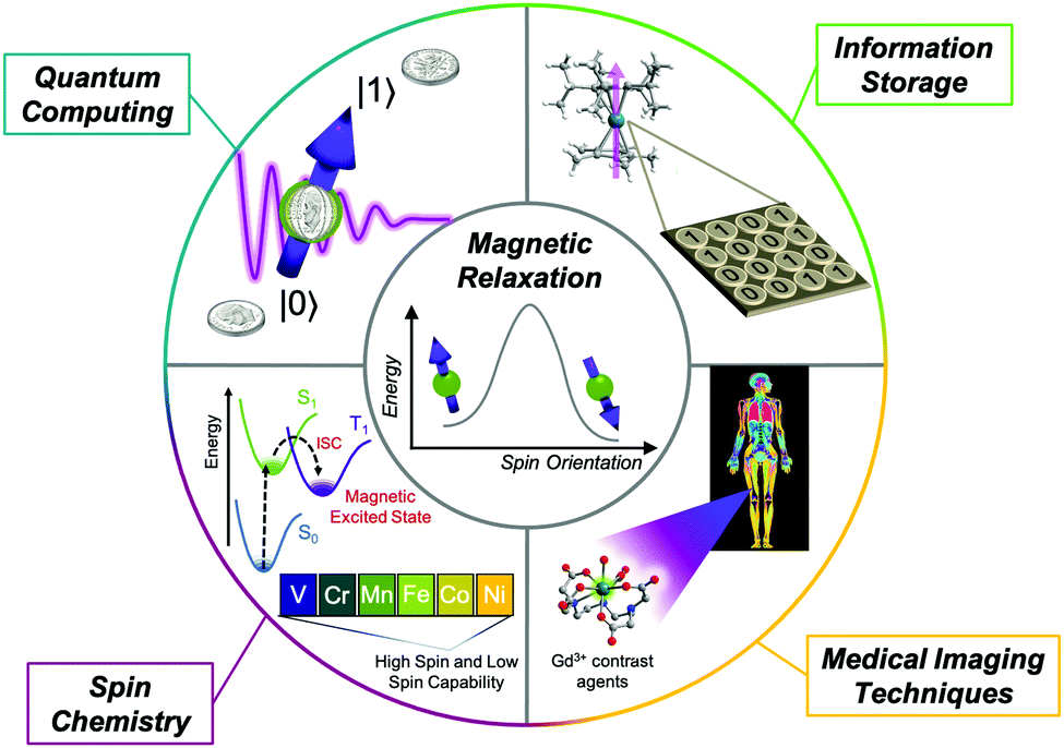 | ||
| Fig. 1 Overview of areas where understanding and designing magnetic relaxation in molecules is important to modern and future technological developments. | ||
A specific magnetic property that is important in the foregoing applications is magnetic relaxation (sometimes called spin relaxation), or the response of the magnetic moment after misalignment from an applied magnetic field (from an MRI scanner or nuclear magnetic resonance spectrometer, for example). A slow relaxation rate permits many important and exciting possibilities, e.g. the storage of information (quantum or classical) in the orientation of the magnetic molecule (here a spin-up orientation could be “0” versus spin-down orientation of “1” in analogy to a simple bit). Slow relaxation rates will also enable certain magnetic resonance spectroscopic experiments (e.g. to noninvasively detect local chemistry) while fast relaxation can make these measurements more challenging. Therefore, there is a clear necessity to understand how to use synthetic design to control and slow down magnetic relaxation – an end goal that many groups are still in pursuit of.
Magnetic relaxation is driven by interaction of the relaxing species with local electronic and magnetic fields. These fields are influenced by intrinsic properties of the molecule. For example, metal-ion identity, spin state, oxidation state, ligand field, and geometry can all affect the relaxation rate of an open-shell metal ion. Extrinsic properties, such as counterion, concentration, temperature, and matrix (e.g. solvent or local chemical surroundings), are also important. Thus, there is considerable overlap between the molecular factors that control magnetic relaxation and those that dictate commonly approached properties by chemists, like reactivity.
Despite this conceptual overlap and the importance of dynamic magnetic properties in many cutting-edge fields, education in magnetic relaxation is typically absent from undergraduate chemical curricula.17–19 As a consequence, concepts in magnetic relaxation can be intimidating for chemistry researchers to utilize in their research. Yet it is precisely these chemists that are needed to make the molecules that drive the observations of new processes, developments of new theories, and surmount the diabolical challenges to designing slow magnetic relaxation processes. This Tutorial Review aims to assist researchers unfamiliar with magnetic relaxation and provide them with an overview of the field in an accessible way. To do so, we draw a direct analogy between the complex quantum mechanical processes of spin relaxation and one of the most intuitive phenomena to the synthetic chemist: the reaction-coordinate diagram (Fig. 2). We focus primarily on metal complexes, though many of the concepts discussed here can be applied to organic radicals as well.
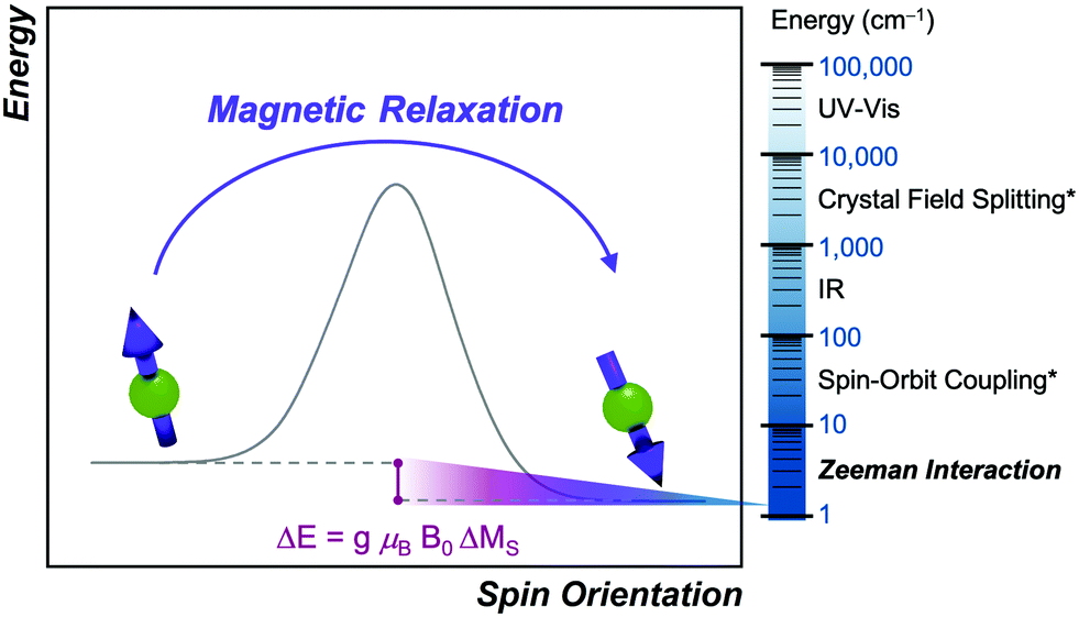 | ||
| Fig. 2 Magnetic relaxation in analogy to a standard reaction-coordinate diagram. Here, the reaction coordinate corresponds to spin orientation, with the products aligned parallel to the applied field and the starting materials aligned against it. The energy difference (ΔE) between the starting materials and products is the Zeeman energy, as defined in the plot. The energy scaling on the right compares the Zeeman interaction to other important energies. Scaling in the reaction coordinate diagram is arbitrary. Asterisks denote energy scaling for 3d transition metals. | ||
A reaction-coordinate picture of relaxation
Magnetic relaxation is the process of a magnetic moment (or a spin) coming to alignment with an applied magnetic field from some other orientation. This misaligned orientation is an excited state while the ground state is when the spin is aligned with the field. For this reason, magnetic relaxation can be thought of analogous to an exergonic reaction that proceeds from relatively high energy reactants (the misaligned orientation) to lower-energy products (the aligned orientation). In the case of a single unpaired electron in an external magnetic field undergoing relaxation (Fig. 2), the starting materials could be “spin up”, corresponding to the spin quantum number . Likewise, the products could be “spin down”, bearing the
  spin quantum number. The relaxation process is then the “reaction” that enables the spin to convert orientation.
There are some important similarities between the relaxation process and a chemical reaction. Just like many reactions, the process of magnetic relaxation is thermodynamically favored.15 There are also often many possible mechanisms by which the system can proceed with relaxation, similar to how many different reaction pathways can exist in a catalytic system. Though there are many of these pathways available to a molecule, again just like with a reaction system, it is the fastest relaxation process that typically proceeds under a given set of conditions. Several relaxation processes have an activation energy, directly analogous to a chemical reaction. However, other relaxation mechanisms can proceed by tunneling through the activation barrier, just like proton-tunneling reactions that can be interrogated through kinetic isotope studies.20 Owing to all the foregoing similarities, it should be no surprise that elucidating the operative magnetic relaxation processes is just as rich and intellectually rewarding as mechanistic investigations of reactions.
There are also some critical differences between magnetic relaxation and a typical chemical reaction. First, the energy difference separating the starting materials and products is extremely small, typically on the order of a few wavenumbers or less so the relaxation process is nearly thermoneutral. This small energy difference is because the energy separating the spin orientations in a typical applied magnetic field (from the “Zeeman” interaction, Fig. 2) is weak. This situation is in stark contrast to the multiple-kcal-energy magnitudes (1 kcal mol−1 = 350 cm−1) separating starting materials and products in a general chemical reaction. Second, the transition states of molecules in the “relaxation reaction” can correspond to high-energy spin orientations, which are discrete and quantized energy levels with mS (or MS if  ) values, or other quantum phenomena entirely. This point highlights a key contrast to a chemical reaction, where a transition state is a transient, high-energy, and distorted molecular geometry. Third, because these transition states are quantized, a given relaxation process does not proceed along a continuous potential-energy curve like molecular transformations, but instead by discrete jumps with emission/absorptions of energy.
We also note that, just like a chemical reaction, the rate of relaxation reflects the slowest step in the operative pathway. Indeed, there are often competing mechanisms, yet the slowest step in the fastest pathway is most important for the observed rate. In this light, the “rate-determining step” for magnetic relaxation is whether the environment can provide the energy to drive the process or accommodate the energy emitted during relaxation.21 This process is in contrast to reactions where rate determining steps involve structural transformations or proton/electron transfers, and possibly isolable chemical intermediates.
The figure of merit for magnetic relaxation is the time constant of the process, the magnetic relaxation time, which is the inverse of the relaxation rate. The timescale of a magnetic relaxation time is highly variable, typically ranging from picosecond to minute timescales. There are two basic types of magnetic relaxation, spin–lattice relaxation, T1, and spin–spin relaxation, T2. Both of these parameters are vital for the applications in Fig. 1. In light of this importance, it is essential that we understand how to control the processes that govern these relaxation times and how they correlate to molecular structure. Below we describe the different relaxation mechanisms that govern these two relaxation times, again in analogy to the basic chemical reaction-coordinate paradigm described above.
Basic molecular spin properties relevant to relaxation
In evaluating the reactivity of a metal complex used in a reaction or as a catalyst, common considerations might be steric congestion or electron abundance/deficiency in the ligand scaffold. Similarly, for coarse-grain prediction of a magnetic relaxation property, there are several key magnetic parameters that are important to consider as a starting point. These parameters are the g factor, hyperfine coupling interactions, and zero-field splitting (Fig. 3). Comprehensive treatments of all the magnetic properties in metal complexes, which are diverse, can be found elsewhere.15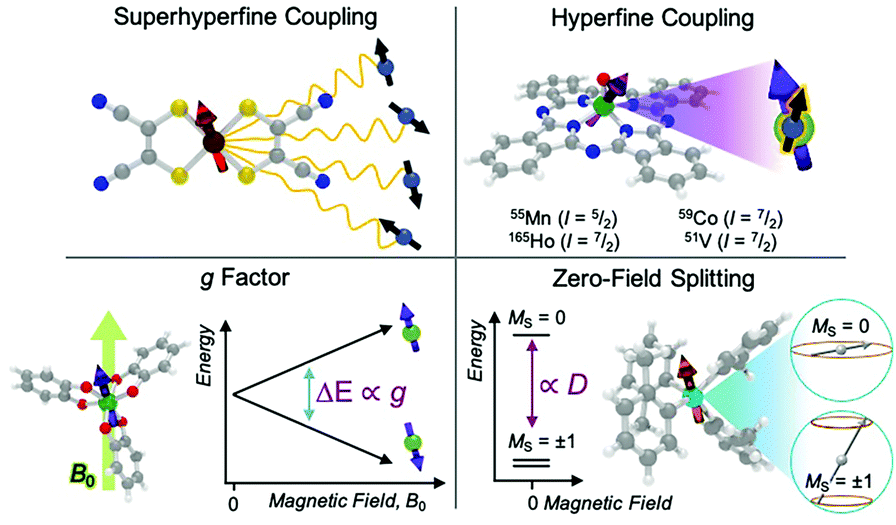 | ||
| Fig. 3 Graphical overview of chemical features that impact relaxation processes. | ||
The first magnetic factor is the electron gyromagnetic ratio, or g factor. Electrons possess an intrinsic angular momentum with a magnetic moment that interacts with an applied magnetic field. The strength (or energy) of this interaction is proportional to the applied magnetic field (B0), the Bohr magneton (μB, a fundamental constant), the mS value of the given spin orientation, and the g factor: E = gμβB0mS. The part relevant to relaxation is the g factor, a proportionality constant that describes the sensitivity of the magnetic moment to an external magnetic field. Simply stated – a larger g factor indicates a larger change in energy between different spin orientations in an applied magnetic field (Fig. 3).
The g factor often gives different values based on the orientation of a molecule in a magnetic field. The g value is often referred to as the g tensor for this point. For an organic radical, g will be close to 2.0023, which is the g factor for a free electron, and relatively independent of orientation. In contrast, metal complexes often have highly orientation dependent g values that can range from 0 to nearly 20 and are often anisotropic (i.e. gx, gy, and gz are all different, x, y, and z here defined with respect to molecular axes). The largest and most anisotropic g factors tend to be found in rare-earth ions and low-coordinate transition metals.22 Generally speaking, anisotropic g values tend to produce faster relaxation rates, though there are many exceptions.
The second important factor is the magnetic interaction between an unpaired electronic spin and a nuclear spin on the same atom. This interaction is known as the hyperfine coupling interaction and has a strength denoted by the hyperfine coupling constant (A) (Fig. 3). An example of this interaction occurs in Co(II) complexes, from the coupling of the magnetic nucleus of 59Co (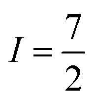 ) and the unpaired electrons. Hyperfine interactions are very similar to J-coupling in proton nuclear magnetic resonance (NMR) spectroscopy. Hyperfine couplings can also be anisotropic, just like the g factor.
Magnetic nuclei are abundant in complexes beyond the spin-bearing ion and are often located in the ligand shell, counterions, and the surrounding matrix (e.g. proton-rich organic solvents,  1H). Magnetic interactions with these latter three classes of nuclei is commonly referred to as “superhyperfine” coupling. Typically, stronger superhyperfine interactions with environmental magnetic species engender faster relaxation rates, though there is nuance to this statement that will be described later.
The final interaction that is noteworthy to highlight, known as the zero-field splitting, is a specific manifestation of spin–orbit coupling in metal ions with spin states greater than  (as a result of bearing two or more unpaired electrons) (Fig. 3). For an electronic spin with
 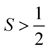 , there are |2S + 1| accessible MS levels. Each MS level corresponds to a different alignment of the electronic spin relative to a molecular axis. A high |MS| value represents a spin precessing tightly around a molecular z axis, or closely aligned with that axis. A low |MS| value, in contrast, is a spin precessing far away from that same axis, commonly represented with perpendicular alignment to z. In the absence of zero-field splitting, or for a light atom (like an
  organic radical), the MS levels are degenerate, or nearly so, at zero applied magnetic field. In the presence of zero-field splitting, which is common for heavy metal atoms (3d, 4d, 5d, 4f, and 5f elements) however, they are not, as shown in Fig. 3.
There are two parameters that describe the zero-field splitting. The first, the axial zero field splitting, or D, splits the energies of |MS| levels away from one another (e.g. it will separate a pair of MS = ±1 levels from MS = 0 levels as in Fig. 3). For first-row transition metal complexes, values of D can range from less than 1 cm−1 to hundreds of cm−1.22 The sign of D causes two limiting cases of MS-level orderings. A positive D indicates a spin where the lowest energy level is MS = 0 or  , depending on whether S is integer (even number of electrons) or half-integer (odd number of electrons). A negative D indicates a spin where the MS levels with largest |MS| are lowest in energy (e.g. MS = ±1 for an S = 1 Cr4+ ion, as shown in Fig. 3). The second parameter, E, the transverse zero-field splitting or rhombic zero field splitting parameter, will cause an energy splitting of MS levels in a pair (e.g., it will split MS = ±1 levels from each other at zero field). The ratio |E/D| is often referred to as the rhombicity.23
The zero-field splitting is important for relaxation because individual MS levels are the starting points, end points, and often transition states of the magnetic relaxation process. Thus, the zero-field splitting parameters directly modify the relaxation rates by dictating the relative energies of all involved steps in a relaxation pathway. The parameters D and E are also a direct result of the electronic structure of the metal complex, meaning that many intuitive molecular features, primarily symmetry and ligand field, can be modified to direct the sign and magnitude of D and E. This fact also means that general correlations between D, E, and relaxation times are challenging to make, and are best discussed on a case-by-case basis.
Spin–lattice relaxation (T1)
Spin–lattice relaxation (also called longitudinal relaxation) refers to relaxation driven by interactions between the molecule and the environment, or “lattice,” that exchange energy. Spin–lattice relaxation specifically describes the process for a spin to relax from a starting spin-up (destabilized) orientation to the spin-down (stabilized) product orientation (Fig. 2). There is an enormous mechanistic diversity in how this process occurs depending on how a magnetic molecule exchanges energy with the lattice.The energy exchanged with the environment during spin–lattice relaxation is in discrete amounts. Here, energy is exchanged through phonons, which are collective, long-range vibrations in a solid, often spanning multiple molecules.24 The availability of phonons in a system is dependent on the temperature of the system and the nature of the surrounding matrix (e.g. a crystalline vs. frozen solvent glass environment).27
The rates of the different mechanisms of relaxation that we discuss below generally follow different temperature, magnetic field, or environmental dependencies. Furthermore, the rates of these processes may be impacted by the lattice just as much as the molecule itself. Thus, in any real system, unraveling the operative mechanisms requires measuring the dependence of the relaxation process on all of these parameters. This process, though applied to dynamic magnetic processes, is therefore comparable to how one might determine the full picture of potential reaction pathways in a catalytic system. Below we give an overview of each of the known mechanisms of spin–lattice relaxation, their relation to the reaction analogy established earlier, and the dependence of the processes on the molecule and environment.
Measurement of T1
Spin–lattice relaxation is measured primarily by two different instruments: a magnetometer such as a magnetic properties measurement system (MPMS), or a pulsed electron paramagnetic resonance (EPR) spectrometer. Magnetometers allow for the study of magnetic relaxation processes across a range of temperatures, time scales and magnetic field strengths with the technique of alternating current (ac) susceptibility. However, the limited frequency range for ac susceptibility measurements (typically 0.01–1500 Hz) means that quickly relaxing systems (T1 < ca. 0.1 ms) can not be easily analyzed with this instrument. An alternative analysis is by pulsed EPR spectroscopy, which can measure T1 through inversion or saturation recovery experiments. This technique can measure much faster relaxation times (T1 ∼ 1 μs lengths), but pulsed spectrometers are far less common than magnetometers. There are some slight differences in the time constant measured by the techniques, because ac susceptibility extracts T1 from bulk magnetization while the EPR experiment is probing a specific transition.25 However, at the microscopic level, the same process is occurring – a spin is flipping during the process of relaxation. We direct the interested reader to several key resources to learn about these techniques in deeper detail.4,26Mechanisms of spin–lattice relaxation
Below we discuss the collection of mechanisms that drive T1 relaxation, starting from those that most closely resemble the reaction-coordinate analogy, then move on to processes that deviate from the analogy and demonstrate the complexity of relaxation phenomena in magnetic molecules.Orbach process
The Orbach process proceeds by excitation from the starting spin orientation to a higher energy spin orientation with energy provided by a phonon. This higher-energy MS level is the effective transition state for the Orbach process. Relaxation then proceeds from this transition state to the lower energy spin orientation by releasing energy (in the form of a phonon) to the lattice (Fig. 4).26,27 For this process to occur, there must be available phonons of the appropriate energy to excite to the transition state. The Orbach process is not limited to a single “transition state” and can involve multiple steps to a higher energy MS level before relaxation via phonon emission.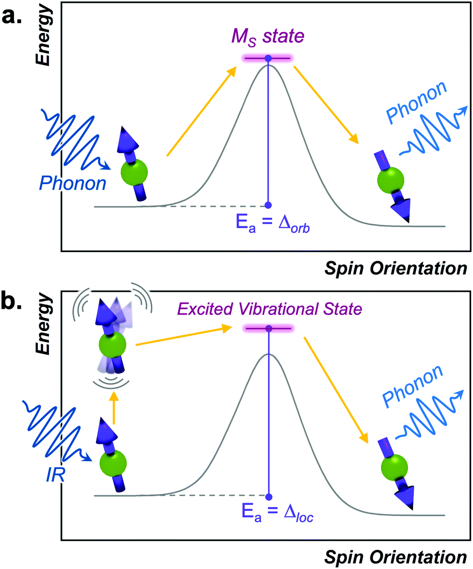 | ||
| Fig. 4 (a) Depiction of the Orbach process in analogy to a reaction-coordinate diagram. The transition state is an actual high-energy MS level for the relaxing spin. (b) Energy profile of the local mode process. Here, discrete vibrations in a molecular species promote the spin to overcome the barrier and enable relaxation. | ||
High-spin metal ions frequently relax via the Orbach process, as other MS levels within the |2S + 1| manifold often serve as transition states. In contrast,  molecules do not show the Orbach process, as there are only two mS levels for an
  system (
 ) (and thus no transition state). The relaxation rate of the Orbach process is described by:
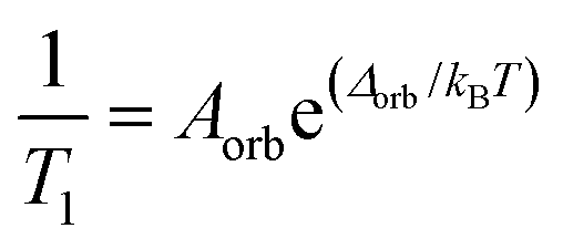 | (1) |
This equation mirrors the form of the Arrhenius law, where 1/T1 is the rate constant. Aorb is the attempt frequency for the Arrhenius description and a larger Aorb means there is higher probability the mechanism will contribute to relaxation. Aorb is determined by several factors: it decreases in magnitude with increasing phonon availability (or energy availability) and generally increases as the activation energy increases.15 Hence, it is challenging to determine Aorba priori on the basis of intuitive molecular considerations. Indeed, the basic theories for understanding relaxation (and the origins of Aorb) are developed for solid state defects, not molecular systems. As such, Aorb is frequently just extracted from experimental data, and is typically found with values of 10−2 to 10−10 s−1.4,15 The term Δorb is the activation energy (Ea) to the MS-level transition state. Finally, note that Aorb is denoted as τ0 and Δorb as “Ueff” or “effective energy barrier” in the single-molecule magnet literature, which tends to focus on these parameters as the key figures of merit.4 An example molecule that exhibits the Orbach process is presented in the state-of-the-art section.
Local mode processes
The local mode relaxation mechanism utilizes discrete vibrations (“local modes”) on a molecule to facilitate relaxation.28,29 Here, incoming energy excites the spin system from the starting configuration to a transition state that is a local vibration. From this transition state, the spin can then relax to the product spin orientation while releasing energy (Fig. 4).30 The process is in some ways like chemiluminescence, where the reaction product (the relaxed spin) is accompanied by an emission of energy, here in the form of a lattice vibration.The temperature dependence of the relaxation rate of the local mode process is described by:
 | (2) |
Direct process
The direct process is the first one we discuss that does not have an activation energy. In this process, a spin directly proceeds from the starting to final orientation because of an energy match between the energy separation of the two levels and a lattice phonon.33,34 Importantly, the process effectively circumvents any possible transition states (Fig. 5). The direct process is analogous to the emission step of phosphorescence in photochemistry, where relaxation from an excited triplet to a ground singlet occurs without an activation energy, with a release of energy in the form of a phonon (a visible photon in the phosphorescence picture). However, unlike for phosphorescence emission, which involves a change in the number of unpaired electrons, the direct process is simply a change in spin orientation for the relaxing species.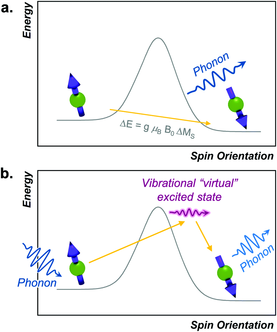 | ||
| Fig. 5 (a) Depiction of the direct process in analogy to a reaction coordinate diagram. The spin flip energy is the Zeeman energy and relaxation emits a single phonon of that energy to the lattice. (b) Depiction of the Raman process in analogy to a reaction coordinate diagram. The “virtual” transition state is a superposition of vibrational states in the solid and is not an actual defined energy level. Relaxation involves two phonons in a simultaneous excitation and deexcitation of the spins, ultimately transferring energy to the environment of an amount equal to the ΔE between the starting and product spin orientations. | ||
The direct process has a distinctive magnetic field and temperature dependence that can enable diagnosis with relaxation studies. Indeed, the rate of relaxation for the direct process is described by the follow equation:
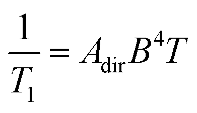 | (3) |
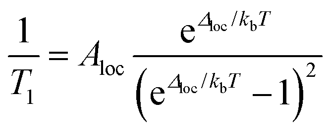
Raman process
The Raman relaxation process is more common at higher temperatures than the direct process. The Raman relaxation process proceeds when a spin system simultaneously absorbs and emits phonons of differing energies. This action is fundamentally different than the direct process, which emits only one phonon, or the Orbach process, which involves successive absorption then emission. The difference in energies between the two phonons of the Raman process must match the difference in energy between the starting and final orientations. The fact that these phonons have defined energies suggests that there is absorption to and from a well-defined transition state. However, for the Raman process, that “state” is a superposition of lattice vibrations and does not actually exist, and is commonly referred to as a “virtual state”15,33 (Fig. 5b). This relaxation mechanism therefore does not have a clear connection to the classical reaction-coordinate picture developed earlier in this tutorial.12 Nevertheless, the observation of the Raman process is incredibly common in relaxation studies. One example of a molecule exhibiting this process is the cobalt complex [Co(acac)2(H2O)2], which demonstrates the Raman process above 3 K when measured by ac susceptibility under ca. 1000 G magnetic fields.38The rate of relaxation via the Raman process is described by the following equation:
 | (4) |
The Raman process produces a characteristic temperature dependence because of the exponent n. In theory, the rate of relaxation should scale with T9 (n = 9) for species with a half-integer spin state and T7 (n = 7) for integer spin state. In practice, however, multiple processes are often active and thus the apparent exponent extracted from fitting variable-temperature T1 data is a non-integer value or ranges down to n = 2 to 3.40 The Raman process commonly occurs at temperatures where the lattice does not have available phonons of sufficient energy to excite the spin system to an actual transition state for the relaxation process. For this reason, this process “undercuts” the barrier, just like the direct process.
Quantum tunneling processes
All previous mechanisms require energy input/release via interacting with the phonon system of the environment. However, there are two processes that circumvent this requirement by tunneling straight through the activation barrier for relaxation. It is for this reason that these processes are referred to as quantum tunneling of the magnetization (QTM) processes (Fig. 6).23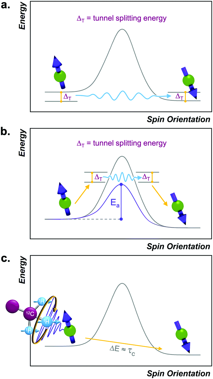 | ||
| Fig. 6 Reaction-coordinate depictions for (a) ground-state and (b) thermally assisted quantum tunneling of the magnetization processes and (c) thermally activated processes. | ||
There are two QTM-based processes. One occurs directly between the starting and final spin orientations, without any input energy, and is referred to as “ground-state” QTM (Fig. 6). This type of tunneling mechanism is operative if there is a magnetic interaction between the wavefunctions of the starting and final spin orientations, which opens a tunnel-splitting energy gap in the barrier (ΔT, Fig. 6). Just like an electron tunnels because its spatial wavefunction can exist on both sides of an impenetrable barrier, the spin wavefunction of a system can exist on both sides of the activation barrier for reorientation. A stronger interaction between the starting and final orientations will generate a larger ΔT and enable more efficient tunneling. Ground-state QTM is most facile near (or at) zero applied magnetic field, because interactions that drive QTM are strongest when the energy difference between the start and endpoint is smallest. Furthermore, the relaxation rate is generally temperature-independent because the tunneling mechanism does not require energy from phonons to ascend over a barrier. Tunneling is typically dominant only at the lowest temperatures, when the available phonons lack sufficient energy to enable any of the other processes. For example, the molecule [Ph4P]2[Co(SPh)4] displays tunneling below 2.5 K when measured by ac susceptibility under zero applied field.41
The second tunneling mechanism, thermally assisted QTM, requires exchange of energy with the lattice (Fig. 6). This mechanism involves an initial promotion (via phonon) of the starting spin orientation to a higher-energy MS level. For the thermally assisted process, this level is below the highest-energy Ms level within a given manifold of an  species (Fig. 6). Once promoted, the system then tunnels through the barrier to another Ms level, from which it can finally relax to the product. The thermally activated QTM mechanism behaves analogously to the Orbach process because of the promotion and phonon emission. However, this mechanism proceeds with an activation energy that is lower than the theoretical maximum defined by the zero-field splitting. An example of this phenomenon is illustrated with the S = 2 species [(TPAtBu)Fe]−, which exhibits a ΔOrb of 65 cm−1, which is lower than the theoretical maximum of 192 cm−1 for this molecule.42
Thermally activated processes
Thermally activated processes are relaxation processes that are driven by thermal motion in the environment, e.g. methyl or amino group rotations, wherein magnetic nuclei are located on the moving structure (Fig. 6). This process is common at higher temperatures, when the surrounding matrix of a magnetic molecule softens to allow physical motion to occur, when they would otherwise be frozen at low temperature.28,33,43 A given local motion will affect relaxation if the correlation time of that motion (τc, or the inverse of the rate of the local motion) approaches the energy difference of the starting/ending orientation (ω, in frequency).43 The rates of thermally activated processes follow this equation: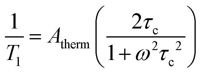 | (5) |
Here, Atherm correlates to the amplitude of the local magnetic field fluctuations from the thermally activated motion (but is generally treated as a weight for this process’ contribution to T1, like Aorb, Aloc, ARam, and Adir), τc‡ is the correlation time of the thermally activated process, and ω is the frequency of the energy gap between the starting/ending spin configurations.43τc is temperature-dependent but depends on the activated motion and molecule, as τc needs to approach 1/ω. As such, there is no diagnostic temperature dependence for this process in the absence of other information about the molecular structure. One example of a molecule that displays this type of thermally activated process is in RbC60 fulleride, where a metal-to-insulator phase transition triggers fast relaxation (measured by pulsed EPR) at ca. 25 K and 3400 G.43
Intrinsic and extrinsic factors that impact T1
There are many chemical and physical factors that impact T1 relaxation in 3d transition metal ions. First, we describe the important (and synthetically tunable) factors for T1 that are intrinsic to molecules then move on to extrinsic parameters that impact T1.Strength and symmetry of the ligand field
The effects of the ligand field on relaxation most commonly manifest through zero-field splitting in high-spin ions. This tendency is for two main reasons. First, the magnitudes of D and E, which are governed by the ligand field, can shift the energies of the MS levels involved in relaxation. Thus, D and E will dictate the activation energies for both the Orbach and thermally assisted QTM mechanisms. Second, a nonzero value of E will induce ground-state QTM as an efficient relaxation pathway. Generally, the magnitudes of D and E are greater when the ligand field for a high-spin metal ion is weaker. However, the dependence of D (both in sign and magnitude) on the ligand field is extremely intricate, and so many exceptions to this rule exist. Furthermore, the magnitude of E is heavily dependent on symmetry. Coordination geometries that have one principal axis of rotation and adhere to nearly idealized uniaxial symmetry tend to have lower-magnitude E parameters and thus, suppressed ground-state tunneling. We refer the reader to excellent reviews of these parameters, which demonstrate the power of molecular design for tuning relaxation processes.12,13,44,45Spin state
The effects of integer (“non-Kramers”) versus half-integer spin (“Kramers”) systems of unpaired electrons are evident most clearly in the QTM relaxation pathways. Here, a species with an integer spin is far more likely to exhibit relaxation by ground-state QTM than a half-integer-spin complex, because the term E is more effective at opening a tunneling gap for integer spin than half-integer-spin species.4 A second place the spin state impacts relaxation is the difference in temperature dependence of the Raman process, as described earlier.Isotopic identity
Many metal ions possess isotopes that have non-zero nuclear spin, e.g.59Co ( , 100% natural abundance) or 165Ho (
 , also 100% natural abundance). The impact of a non-zero nuclear spin is primarily observed at zero field, low temperatures, and primarily affects quantum tunneling mechanisms.46 The origin of this effect is the hyperfine coupling to the metal-ion nuclear spin, which can open a tunneling gap and increase the rate of QTM.
Spin–orbit coupling
Spin–orbit coupling (SOC) is an intrinsic property of a molecule. This fundamental electronic structure feature is broadly important in dictating relaxation, but has two different effects, generally depending on whether relaxation occurs at high temperature or low temperature. The high temperature impact is because the SOC interaction ties the energies of the MS levels (e.g. potential activation energies for the Orbach process) directly to the spin-bearing orbital energies of the metal ion. Consequently, small changes in the structure of a molecule (e.g. from a vibration that modulates metal–ligand bond distances) impact the spin-bearing orbitals, when then modulate the MS-level energies via the SOC to facilitate relaxation. The stronger the SOC for a given system, the more efficient this effect, and the shorter T1 tends to become. For this reason, light-element species, e.g. organic radicals, tend to have T1 values (often μs) that are longer at higher temperature than metal-ion systems. At lower temperature, the effect of a large SOC is different, particularly if the Orbach mechanism is active. In this case, a large SOC can push transition states to higher energies, enhancing the activation energy and ultimately slowing relaxation. The Dy-containing molecule in the state-of-the-art section later in the manuscript is a prime example of this point.The importance of the SOC also means that the relaxation time can be dependent on precisely what orbital an electron resides in. Indeed, this effect is seen for the [V(C6H4O2)3]2−versus [VO(C6H4O2)2]2− molecules, which possess a single d electron in the dz2versus dx2−y2 orbital, respectively. T1 is different by approximately an order of magnitude between these two molecules owing to this difference.47–49
Local magnetic species
The local magnetic species surrounding a molecule (the “spin bath”) also exert important effects on relaxation. This factor is readily altered by the chemist, who can choose, for example, to co-crystallize a molecule of interest with other molecules or dilute by dissolution in different organic solvents.4 These studies show that relaxation times generally increase when local magnetic content decreases, specifically the concentration of open-shell molecules. This general observation is because the presence of nearby magnetic units can hasten several of the above relaxation processes. For example, magnetic coupling to nearby electron spin systems will produce discrete spin levels that are relatively low-lying above the energies of the starting/ending spin orientations. Thus, the activation energy is lowered, and the relaxation rate accelerates via an Orbach process. Another common observed impact is through quantum tunneling, wherein proximate magnetic species enable the ground state QTM via a tunneling gap created by dipolar interactions.Temperature
Temperature is one of the main extrinsic mechanisms of controlling relaxation. A given spin system will relax via the most efficient mechanism available. Thus, over a given temperature regime, one process is typically dominant, and cooling/heating the system can transition the system to relaxation via a different mechanism. The exact ordering of these domains with temperature is highly dependent on the studied system. Nevertheless, a general ordering scheme is still possible. Ground-state QTM and the direct process are often observed at the lowest temperatures, where high-energy phonons are unavailable. A system will then usually transition to a regime where the Raman process is active upon warming. With further increasing temperature, where high-energy phonons become available in the solid, the Orbach process (or the analogous thermally assisted QTM) will typically take over. At even higher temperatures, local-mode and thermally activated mechanisms become active. A complete picture of magnetic relaxation for a molecule requires scanning an abundance of temperatures, just like understanding the kinetics of a chemical reaction.Magnetic field
The applied magnetic field is the second most-commonly varied extrinsic factor for studying relaxation. Most relaxation processes exhibit a field dependence, because the magnetic field will vary the energies of the starting and final spin orientations. The only relaxation process with a rate that has a field dependence explicitly written into the equation is the direct process, which displays a B4 field dependence. However, in the case of processes that involve an MS-level transition state, the applied field can also vary the energy of the transition state, thereby modifying the activation energies and rates, though this impact is relatively small. A changing applied field can also affect the efficiency of the thermally activated process, by modulating the difference between the ΔE for the starting/ending spin configurations and the correlation times of environmental motions. Applied fields are also enormously impactful in the quantum tunneling, as they split the MS levels nominally involved in tunneling, effectively killing the process and inducing slower magnetic relaxation. The effect of a magnetic field is much stronger on the ground-state tunneling process than the thermally assisted one, as larger MS levels have energies that are more sensitive to changes in the magnetic field. The foregoing discussion justifies the widespread nature of using variable fields for studying relaxation: it can enhance T1 by orders of magnitude and is thus a powerful handle for optimization.In summary, there are many dials available to the experimentalist to turn when controlling the operative T1 processes. However, the foregoing points are not the only factors that affect T1. Indeed, there are many other effects stemming from specifics of measurement. We direct the enthusiast to further reading for deeper information.15
The need for benchmarking
Frequently, a molecule will exhibit different relaxation processes depending on the aforementioned extrinsic factors. Because it is often too time-consuming to measure relaxation rates under every conceivable condition, the picture of magnetic relaxation in a molecule is often incomplete, and sometimes magnetic relaxation mechanisms are misassigned. Thus, numerical comparisons of the impacts of the foregoing extrinsic/molecular features can be quite challenging. We contend that a larger discussion about benchmarking relaxation parameters is desperately needed in this field to overcome this difficulty and pave the way to true understanding.Spin–spin relaxation (T2)
Spin–spin relaxation, or T2, describes relaxation of a magnetic moment oriented in the plane perpendicular to the applied magnetic field (Fig. 7). The spin–spin relaxation time is one of the key figures of merit for quantum bits (“qubits”) in quantum computing, quantum sensing, and other quantum-information based fields.2,11 The given orientation-based description of T2 is useful for instruction but note: the orientation of a spin is quantized and thus can only orient up or down in a magnetic field. The sideways depiction of the spin is in reality a unique quantum state known as a spin superposition, existing as both spin-up and spin-down orientations simultaneously. This quantum state is the cornerstone of the computational advantages for spin-based qubits.2 A spinning-coin based analogy of the superposition is depicted in Fig. 7. Here, a spinning coin is neither heads nor tails but both simultaneously. Similarly, the spin up or spin down orientations are heads or tails, while the superposition is both. | ||
| Fig. 7 Reaction-coordinate depiction of spin–spin relaxation. Spin up and spin down are shown to illustrate that the superposition can collapse to either spin-up or spin-down states. Coins depict the commonly used analogy that a spinning coin is a superposition of both heads and tails, or spin-up and spin-down state, respectively. | ||
In general, the superposition is an extremely delicate state and will decay into its constituent states very quickly after it is generated. The lifetime of this decay is the spin–spin relaxation time, T2. These values can range from very short (on the order of a few nanoseconds) to extremely long (on the order of milliseconds). For many applications of qubits, T2 needs to be 100 μs, and pursuit of ever-larger T2 values is a growing area of work.1,2,50 This time constant is known by several other names in the literature: coherence time, transverse relaxation time, and phase memory relaxation time. We refer the interested reader to further references for the key differences between them.15,33 In general, however, these terms are used interchangeably to describe the same relaxation process. In this review, we will use the term “spin–spin relaxation time” and T2 to describe all forms of this type of relaxation.
The spin–spin relaxation process
The process of spin–spin relaxation is fundamentally different than spin–lattice relaxation because of the superposition state, which does not require thermal activation to relax. Instead, any interaction of the superposition with the environment that perturbs the energy of the spin will initiate relaxation. We refer the interested reader to deeper descriptions of the spin–spin relaxation process and superposition collapse,33,51 as the ultimate goal here is to understand how local chemistry controls T2. Importantly, because there are many ways that the environment can interact with the spin superposition, there are likewise many factors that affect T2.The immediate question, then, is how to apply the reaction-coordinate paradigm to understanding T2. However, the typical reaction-coordinate diagram is insufficient to describing the process, because the superposition is, in some sense, the transition state itself. As such, the activation energy is the input from the experimentalist, often with pulses of microwaves and the technique of pulsed EPR, to generate the superposition in the first place (Fig. 7). This fact is why T2 relaxation does not follow the typical temperature-dependent rules that T1 does. As one final point, T2 is often much faster than T1. Whereas T1 can approach second- and minute-long magnitudes for molecules, in most cases T2 is at most hundreds of microseconds (rarely so), and more commonly tens of microseconds or less.11
Measurement of T2
The most common way of measuring the T2 of a magnetic molecule is through the use of a pulsed EPR spectrometer. This instrument can apply a brief pulse of microwaves (typically 10-to-100 ns in length) to “tilt” the spin perpendicular in the applied magnetic field and generate the superposition. Then, after a delay, a second pulse of microwaves is applied, which triggers an emissive magnetic response, a Hahn echo, from the superpositions that have not decayed since the initial pulse. The time dependence of the echo intensity then provides a direct measurement of the lifetime of the superposition, which is T2. T2 values typically have to be at least tens of nanoseconds in length to measure with commercial instrumentation. We direct the interested reader to several key volumes with more thorough descriptions of the techniques and instrumentation for analyzing T2.33Intrinsic and extrinsic factors that impact T2
There are many different ways that the local chemical environment will affect T2 (Fig. 8). For metal complexes, it is important to note that the “local environment” does not exclude the molecule itself. Indeed, specific molecular features, as detailed below, can and do commonly control T2 by imposing specific local environmental effects. First, as for the T1 section, we describe specific molecular features that control T2 that can be manipulated by the synthetic chemist. Then we cover a select number of important extrinsic tunable features in the local environment that will affect T2. The following description is not exhaustive of all of the features that can affect T2, some of which can be induced by details of the measurement process itself. We refer the reader to other sources for descriptions of these effects.15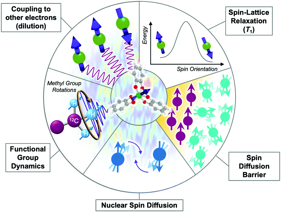 | ||
| Fig. 8 Graphical depiction of intrinsic and extrinsic processes that affect T2. Processes that hasten T2 relaxation via the creation of noise in the local magnetic field possess a “noisy” background. | ||
Electronic structure
The main ways that the electronic structure of a metal ion affects T2 is by enhancing or suppressing environmental interactions. High-spin states (and the oxidation states and ligand fields that enable such spin configurations) tend to have shorter T2 values because the larger magnetic moments of these spins display stronger dipolar interactions with environmental magnetism. This tendency is why molecular systems with the longest T2 values tend to be ions, e.g. V(IV) and Cu(II).48,52 In the final section of this review, we detail two additional cutting-edge methods of manipulating electronic structure to suppress environmental interactions.
The second way that electronic structure will affect T2 is through manipulating spin–lattice relaxation. Spin–lattice relaxation is the upper limit of T2 for a molecule, because relaxation in the plane perpendicular to the magnetic field will be rapid if the spin is also rapidly realigning with the applied magnetic field direction.26 When T1 is short enough, T2 is effectively controlled by all of the molecular factors described in the T1 section. At the lowest temperatures, however, T1 is usually orders of magnitude longer than T2. In these situations, T1 does not limit T2, but with increasing temperatures, T1 will frequently shorten, eventually becoming the dominant contributor to T2 relaxation.2,15
Functional groups, counterions, and their dynamics
Functional groups are important for governing T2, like for many other chemical properties of molecules. However, those functional groups have to exert a chaotic, noisy fluctuation in the local magnetic field to affect T2. For example, the conventional “steric bulk” from a tert-butyl group will have an influence on a metal-ion T2 not by impeding substitution-based reactivity, but because of a superhyperfine interaction with the nine magnetic protons (1H,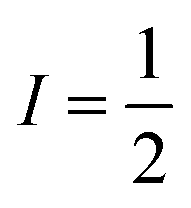 , μ = 2.79μN where μ is the nuclear magnetic moment in units of μN, the nuclear magneton) contained in the functional group.
There are two key points to make about the impacts of ligand and counterion-based magnetic nuclei. First, the motion of magnetic nuclei on functional groups in ligands and functional groups, such as rotation (e.g. in methyl groups), will generate potent changes in the local magnetic field that will shorten T2. Molecular motion shows its greatest effect on T2 when the rate of a given motion is on the timescale of the measurement of T2 and the dynamic group is closer to the spin.53 The impact of motion on T2 does not have a specific temperature dependence like T1, but instead will vary substantially at the temperatures where the timescale of a given motion approaches that of measurement. Second, the type, relative position, and number of magnetic nuclei on the ligand/counterion are all tunable handles to adjust T2. For example, substitution of proton nuclei with lower-magnetic-moment nuclei (e.g.2H, I = 1, μ = 0.86μN) will result in longer T2 values because those substitutions suppress the amplitude of fluctuations in the local magnetic field. Finally, modifying the relative interactions between magnetic nuclei and the magnetic ion by varying the substitutional pattern on ligands, or changing the distance separating the metal ion and the magnetic nuclei, will also affect T2. There is considerable power in manipulating T2via molecular design through these species, though there is much to learn in this area.
Librational motion and orientation dependence
In many molecules, the relative orientation of the molecule to an applied magnetic field will affect the T2 magnitude. This sensitivity stems from small molecular motions called librations (wagging/stretching of an entire molecule, not individual functional-group vibrations) that can occur at low temperatures. These librations will slightly change the orientation of the molecule in the applied magnetic field. If the g factor is anisotropic, as it is for many molecules, then the librations perturb the interactions with the applied magnetic field. This change in interaction drives T2 relaxation. For many species, T2 is greatest where a particular x, y, or z axis of the molecule is orientated parallel to the applied field, as slight changes at these orientations produce relatively small changes in the interaction with the applied field than “off-axis” orientations. There are two important practical outcomes of this effect. First, there is no single T2 for a molecule, instead, a given molecule will often exhibit multiple different T2 values depending on its orientation relative to in an applied external magnetic field. Second, because of the orientation dependence, orientation is a critical design concern for any proposed molecule-based quantum computing architecture, specifically surface-mounted ones.54Local magnetic species
Fluctuations in local magnetism induced by other molecules in the environment also hasten T2 relaxation. The strongest impacts come from proximate open-shell molecules, which exert their own local magnetic fields to hasten T2. The impact of local magnetic species is also more prominent when there are more of them, and T2 can generally be observed to decrease with increasing concentration of open-shell species.15,33 Conversely, dilution increases T2 and thus most reported T2 times for molecular complexes are measured in millimolar (or less) concentrations.2,52,53,55,56A separate source local magnetic species is the collection of magnetic nuclei on surrounding molecules and matrix. The impacts of environmental nuclei can exert similar impacts on T2 as nuclei in the ligand-shell. Hence, dynamic motion such as methyl rotations in the local matrix will shorten T2 just as if it were part of the metal complex itself. A second mechanism through which nuclei can generate local magnetic noise and shorten T2 is nuclear spin diffusion. Recall that the chemical shift of a magnetic nucleus is the energy required to flip that magnetic nucleus in a magnetic field. Spin diffusion occurs when two oppositely oriented nuclear spins (with identical chemical shifts) undergo a simultaneous flip, a “flip flop”, which produces changes to the local magnetic field (Fig. 8, bottom).
Nuclear spin diffusion is energy conserving, meaning that it cannot be frozen out by cooling to low temperatures, in contrast to other factors that affect T2. Therefore, nuclear spin diffusion tends to become the main contributor to T2 at the lowest temperatures. The impact of this process can be minimized somewhat if the environment is full of lower-moment magnetic nuclei, e.g. a frozen deuterated solvent matrix instead of a protiated one.2,52,56
Spin diffusion barrier
The requirement of matching chemical shifts between spin-diffusion-active nuclei generates a unique feature known as the spin diffusion barrier, which surrounds a relaxing open-shell molecule. Environmental magnetic nuclei interact with the magnetic molecule and that superhyperfine coupling strength grows as the magnetic nuclei approach the electronic spin. At a certain radius, even adjacent nuclei experience substantially different strengths of these superhyperfine interactions. As a consequence, the two nuclei now have significantly different chemical shifts from each other and the other magnetic nuclei of the bath. Spin diffusion is thus deactivated for nuclei in close proximity to the electron, even if the two nuclei are right next to each other. Consequently (and counterintuitively) nuclei that are the closest to an electronic spin will not generate substantial fluctuations in the local magnetic field to shorten T2. The radius at which the T2-shortening effect of magnetic nuclei is deactivated is the spin diffusion barrier.58 Existing studies place the edge of the barrier at about 3–10 Å.57,59 However, the actual radius is dependent on the system, and does not need to be spherical.2,60 Finally, the barrier also precludes spin diffusion as a mechanism by which the hyperfine coupling to a metal-ion nuclear spin will impact T2.61State of the art in molecular magnetic relaxation
The length of the relaxation time for a system directly translates into potential utility. For example, realizing a long T1 is a path toward storing and processing information in a system,13 as well as controlling environmental 1H dynamics for magnetic resonance imaging.62 Producing long T2 values enables quantum information processing52 and enables the performance of advanced magnetic resonance detection protocols, as could be leveraged in, e.g. electron paramagnetic resonance imaging.63 Below we highlight the forefront of this area of work, describing how the combined use of synthetic chemistry and electronic structure design strategies are producing new pathways to slowing magnetic relaxation.Complexes with slow spin–lattice relaxation
One prominent class of molecular species with long spin–lattice relaxation times, single molecule magnets, features a single metal ion (transition-metal or lanthanide) with carefully crafted ligand shells to facilitate a long T1. Many of these design strategies rely on controlling the activation energies of spin–lattice relaxation through the Orbach or thermally assisted QTM process and suppressing the non-thermally activated processes. With a suitably high activation energy and the absence of these other processes, one may expect sufficiently long relaxation to enable information storage in a molecular magnetic moment. In pursuit of this goal, in 2017, Layfield, Chilton, Mills, and coworkers reported new Ln-based metallocene complexes that show a slow relaxation process up to and above liquid nitrogen temperatures (Fig. 9).20,64 Analyses of the temperature dependence of T1 in these species revealed that one molecule, [(CpiPr5)Dy(Cp*)]+, exhibited an activation energy for relaxation of 1541(11) cm−1 for a thermally assisted QTM process, the highest reported value for any molecule. There are two key aspects of the molecule that enable this remarkable observation. First, the molecule possesses a Dy3+ ion, which leverages a large spin state and spin–orbit coupling to produce a large potential activation energy. The spin orbit coupling in particular leads to a 6H15/2 term ground state and magnetic orientations that are described with MJ values up to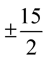 (stemming from J = L + S, where J is the total angular momentum, L the orbital angular momentum, and S the spin).44 Second, the species also possesses a highly pseudo-axial molecular symmetry. These two properties suppress tunneling in the ground state and lower lying levels. The result is a thermally assisted tunneling mechanism that is nearly the maximum possible activation energy for the molecule.
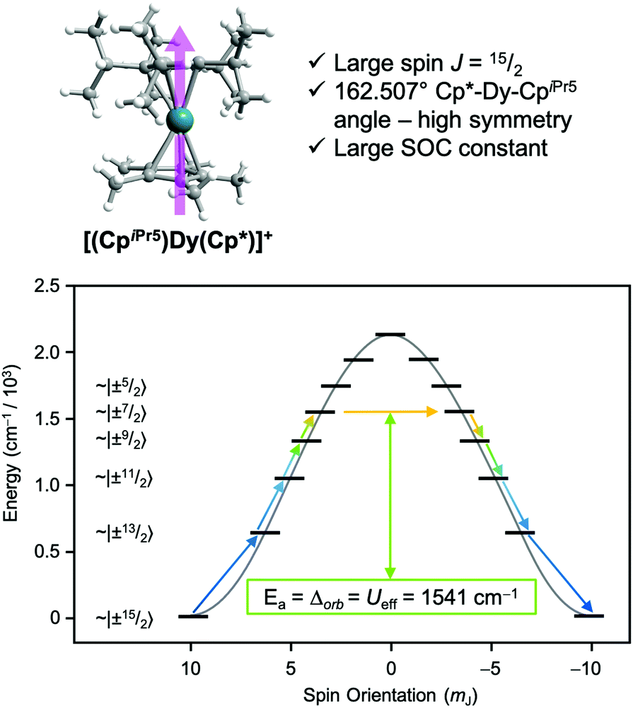 | ||
Fig. 9 Recent ground-breaking system for targeting a long T1. The highly axial geometry of the metal complex suppresses tunneling, which combines with the high spin state and large spin–orbit coupling to enable an exceptionally high activation energy to relaxation. Cp* = pentamethylcyclopentadiene; CpiPr5 = pentaisopropylcyclopentadiene. The levels in the bottom plot are labeled in “ket” notation, which here simply give the MJ values of the 6H15/2 Dy3+ ion, which reach up to 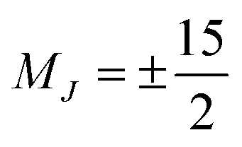 . . | ||
Complexes with slow spin–spin relaxation
Long T2 values are common for open-shell defects in solid-state materials like the nitrogen vacancy center in diamond65 or the double-vacancy site in silicon carbide.66 All of these species exhibit extremely large T2 values (∼1 ms) because isotopic enrichment removes all environmental nuclear spins. Metal complexes are emerging as powerful alternative platforms to understand how to lengthen superposition lifetimes using synthetic chemistry, a strategy that is substantially more challenging in the solid state.Of these, first-row transition metal complexes hold recent records for the longest spin–spin relaxation times. In 2015, Freedman and coworkers demonstrated the impact of using synthetic design to achieve near-complete removal of nuclear spins from the coordination shell of a metal ion. The resulting molecule, (d20-Ph4P)2[V(C8S8)3], uses nearly nuclear-spin free ligands (12C: I = 0, 98.9%; 32/34/36S: I = 0, 99.25%), deuterated counterions, and a remarkable solubility in CS2, a relatively nuclear spin-free solvent. Together, these factors create a magnetically quiet environment, and hence a groundbreaking, millisecond T2 is observed (Fig. 10). This finding (the first for a metal complex) shows that controlling the properties of magnetic nuclei in the environment is critical to lengthen T2, but there is much to learn about the exact role of ligand-based nuclei, and cutting-edge efforts reflect that.48,53
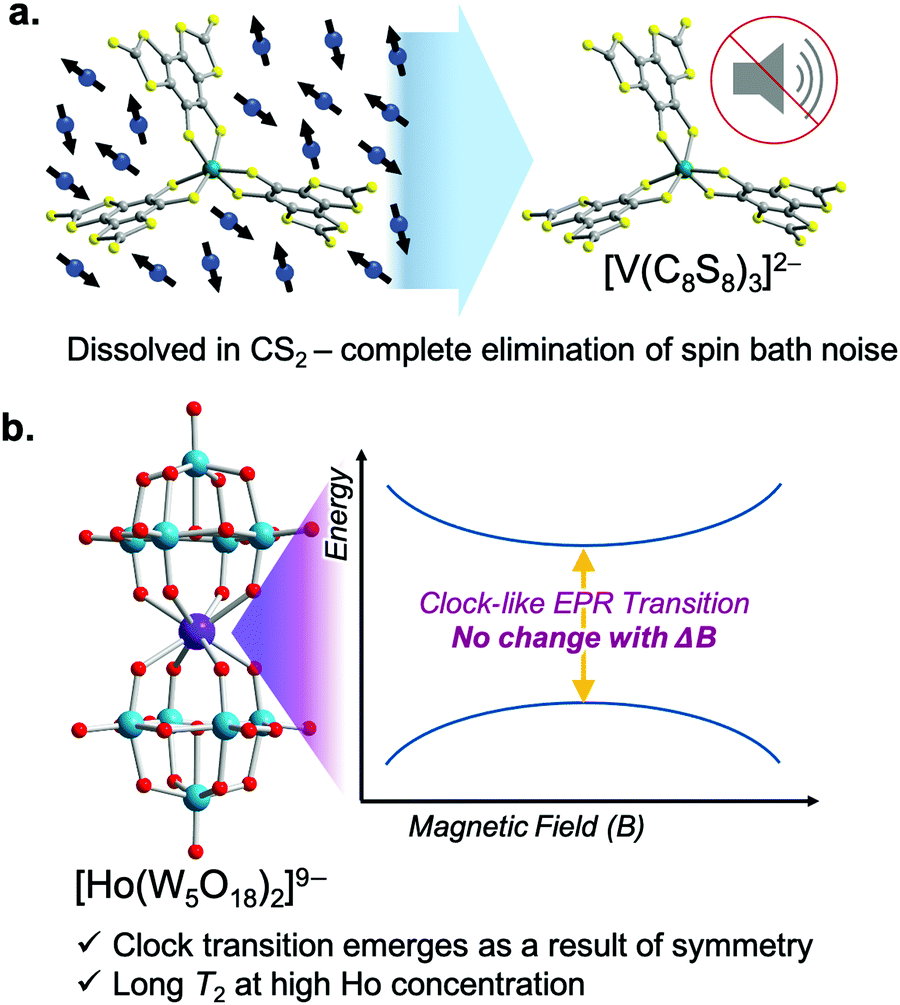 | ||
| Fig. 10 State-of-the-art molecules for lengthening T2. (a) [V(C8S8)3]2− is a predominantly nuclear-spin free complex that displays millisecond T2 values when dissolved in the nuclear-spin-free solvent CS2. (b) [Ho(W5O18)2]9− exploits an almost perfect D4 molecular symmetry to generate a clock-like EPR transition. These transitions have zero change in frequency with respect to changes in local magnetic field, and thus yield long T2 values. | ||
Another exciting strategy to lengthen T2 is to design electronic structures that suppress environmental sensitivity. One method to do so is to create an EPR transition at an avoided-crossing point (Fig. 10). An avoided crossing point is where two MS values would cross in energy at a given magnetic field. For an avoided crossing, however, there is an interaction between the wavefunctions of the MS levels that strengthens as the levels become closer in energy. As a result, the MS levels never actually cross and instead bow away from each other with increasing magnetic field. The result is an energy gap that is accessible with EPR spectroscopy. However, the transition is unconventional as the energies of the MS levels (MJ in the case of the Ho3+) are field-independent at the crossing point. The field independence of the energies translates into a relative immunity toward local magnetism, and the superposition created at the avoided crossing point is consequently relatively long-lived. In fact, this mechanism for designing environmental immunity engenders the extraordinary frequency stability of the time-keeping transition of an atomic clock. It is for this reason that the EPR transition is “clock-like”. In the case of the molecule shown in Fig. 10, the symmetry, orbital angular momentum, and crystal field of the Ho3+ are what create the clock transition. However, other magnetic interactions in molecules can be used to create a clock transition, e.g. the hyperfine interaction.67 It remains to be seen if this strategy will be able to achieve the near-millisecond T2 values in molecules reported by the nuclear-spin-free strategy. Nevertheless, these studies represent a fascinating and rare intersection of coordination chemistry and atomic-clock physics.
Outlook
Magnetic molecules are promising components of next-generation applications spanning from quantum information processing to magnetic resonance imaging. But to realize that potential, we need a comprehensive understanding of how molecular structure and the environment control magnetic relaxation. In this review, we contextualized the relaxation process in a new analogy to a reaction-coordinate diagram, which enabled us to intuit relaxation phenomena in an accessible manner.The question then is, where to next? There are of course many exciting directions, and we touched on a select few of these in the last section. We highlight one final area of particular opportunity: studying relaxation in highly magnetic and dynamic environments. Indeed, many of the proposed applications for magnetic metal complexes require long relaxation times in proton-rich biological environments, room-temperature solutions, or the stray-magnetic-field-rich interiors of electronic devices. Yet, as touched on herein, current studies of magnetic molecules focus almost exclusively on electron- and nuclear-spin-free conditions to suppress magnetic noise and very low temperatures to freeze out structural dynamics. These studies revealed that extraordinarily long relaxation times are achievable. One pressing goal, then is the discovery of how to translate those proof-of-concept observations into noisy conditions. We are excited to see, then, more fundamental studies into controlling the interactions between spin baths and molecules via structural design.
Conflicts of interest
There are no conflicts to declare.Acknowledgements
We thank C. D. Charles and D. A. Corbin for helpful feedback. We thank the NSF (CHE-1836537), the NIH (R21EB027293), and Colorado State University (CSU) for financial support. CSU acknowledges, with respect, that the land the university is on today is the traditional and ancestral homelands of the Arapaho, Cheyenne, and Ute Nations and peoples. I. P. M. is supported by the National Science Foundation Graduate Research Fellowship Program under Grant No. (006784-0002).References
- G. Aromí, D. Aguilà, P. Gamez, F. Luis and O. Roubeau, Chem. Soc. Rev., 2012, 41, 537–546 RSC.
- M. J. Graham, J. M. Zadrozny, M. S. Fataftah and D. E. Freedman, Chem. Mater., 2017, 29, 1885–1897 CrossRef CAS.
- A. Gaita-Ariño, F. Luis, S. Hill and E. Coronado, Nat. Chem., 2019, 11, 301–309 CrossRef PubMed.
- D. Gatteschi, R. Sessoli and J. Villain, Molecular Nanomagnets, Oxford University Press, Oxford, New York, 2006 Search PubMed.
- J. Wahsner, E. M. Gale, A. Rodríguez-Rodríguez and P. Caravan, Chem. Rev., 2019, 119, 957–1057 CrossRef CAS PubMed.
- G. Tircs and Z. Baranyai, The Chemistry of Contrast Agents in Medical Magnetic Resonance Imaging Stability and Toxicity of Contrast Agents, John Wiley & Sons, 2013 Search PubMed.
- M. C. Heffern, L. M. Matosziuk and T. J. Meade, Chem. Rev., 2014, 114, 4496–4539 CrossRef CAS PubMed.
- A. L. Buchachenko and V. L. Berdinsky, Chem. Rev., 2002, 102, 603–612 CrossRef CAS PubMed.
- D. Aravena and E. Ruiz, Dalton Trans., 2020, 49, 9916–9928 RSC.
- S. Brooker, Chem. Soc. Rev., 2015, 44, 2880–2892 RSC.
- E. Coronado, Nat. Rev. Mater., 2020, 5, 87–104 CrossRef.
- S. T. Liddle and J. van Slageren, Chem. Soc. Rev., 2015, 44, 6655–6669 RSC.
- G. A. Craig and M. Murrie, Chem. Soc. Rev., 2015, 44, 2135–2147 RSC.
- L. Bogani and W. Wernsdorfer, Nat. Mater., 2008, 7, 179–186 CrossRef CAS PubMed.
- L. J. Berliner, S. S. Eaton and G. R. Eaton, Distance Measurements in Biological Systems by EPR, Springer, US, 2000 Search PubMed.
- In Vivo EPR (ESR): Theory and Application, ed. L. J. Berliner, Springer, US, 2003 Search PubMed.
- B. A. Reisner, S. R. Smith, J. L. Stewart, J. R. Raker, J. L. Crane, S. G. Sobel and L. L. Pesterfield, Inorg. Chem., 2015, 54, 8859–8868 CrossRef CAS PubMed.
- J. R. Raker, B. A. Reisner, S. R. Smith, J. L. Stewart, J. L. Crane, L. Pesterfield and S. G. Sobel, J. Chem. Educ., 2015, 92, 980–985 CrossRef CAS.
- L. J. Fox and G. H. Roehrig, J. Chem. Educ., 2015, 92, 1456–1465 CrossRef CAS.
- F.-S. Guo, B. M. Day, Y.-C. Chen, M.-L. Tong, A. Mansikkamäki and R. A. Layfield, Science, 2018, 362, 1400–1403 CrossRef CAS PubMed.
- L. Tesi, A. Lunghi, M. Atzori, E. Lucaccini, L. Sorace, F. Totti and R. Sessoli, Dalton Trans., 2016, 45, 16635–16643 RSC.
- J. M. Frost, K. L. M. Harriman and M. Murugesu, Chem. Sci., 2016, 7, 2470–2491 RSC.
- D. Gatteschi and R. Sessoli, Angew. Chem., Int. Ed., 2003, 42, 268–297 CrossRef CAS PubMed.
- M. Vallone, Phys. Status Solidi B, 2020, 257, 1900443 CrossRef CAS.
- M. S. Fataftah, M. D. Krzyaniak, B. Vlaisavljevich, M. R. Wasielewski, J. M. Zadrozny and D. E. Freedman, Chem. Sci., 2019, 10, 6707–6714 RSC.
- A. Schweiger and G. Jeschke, Principles of Pulse Electron Paramagnetic Resonance, Oxford University Press, 2001 Search PubMed.
- A. Lunghi, F. Totti, R. Sessoli and S. Sanvito, Nat. Commun., 2017, 8, 14620 CrossRef PubMed.
- Y. Zhou, B. E. Bowler, G. R. Eaton and S. S. Eaton, J. Magn. Reson., 1999, 139, 165–174 CrossRef CAS PubMed.
- D. W. Feldman, J. G. Castle and J. Murphy, Phys. Rev., 1965, 138, A1208–A1216 CrossRef.
- P. G. Klemens, Phys. Rev., 1962, 125, 1795–1798 CrossRef.
- C. B. Harris, R. M. Shelby and P. A. Cornelius, Phys. Rev. Lett., 1977, 38, 1415–1419 CrossRef CAS.
- N. V. Vugman and M. R. Amaral, Phys. Rev. B: Condens. Matter Mater. Phys., 1990, 42, 9837–9842 CrossRef PubMed.
- D. Goldfarb and S. Stoll, EPR Spectroscopy: Fundamentals and Methods, John Wiley & Sons, 2018 Search PubMed.
- J. Murphy, Phys. Rev., 1966, 145, 241–247 CrossRef CAS.
- A. Abragam and B. Bleaney, Electron Paramagnetic Resonance of Transition Ions, Oxford University Press, Oxford, New York, 2012 Search PubMed.
- K. J. Standley, Electron Spin Relaxation Phenomena in Solids, Springer, US, 1969 Search PubMed.
- A. J. Fielding, S. Fox, G. L. Millhauser, M. Chattopadhyay, P. M. H. Kroneck, G. Fritz, G. R. Eaton and S. S. Eaton, J. Magn. Reson., 2006, 179, 92–104 CrossRef CAS PubMed.
- S. Gómez-Coca, A. Urtizberea, E. Cremades, P. J. Alonso, A. Camón, E. Ruiz and F. Luis, Nat. Commun., 2014, 5, 4300 CrossRef PubMed.
- W. M. Rogers and R. L. Powell, Tables of Transport Integrals, U.S. Government Printing Office, 1958 Search PubMed.
- L. Gu and R. Wu, Phys. Rev. B, 2021, 103, 014401 CrossRef CAS.
- J. M. Zadrozny and J. R. Long, J. Am. Chem. Soc., 2011, 133, 20732–20734 CrossRef CAS PubMed.
- W. H. Harman, T. D. Harris, D. E. Freedman, H. Fong, A. Chang, J. D. Rinehart, A. Ozarowski, M. T. Sougrati, F. Grandjean, G. J. Long, J. R. Long and C. J. Chang, J. Am. Chem. Soc., 2010, 132, 18115–18126 CrossRef CAS PubMed.
- V. A. Atsarkin, V. V. Demidov and G. A. Vasneva, Phys. Rev. B: Condens. Matter Mater. Phys., 1997, 56, 9448–9453 CrossRef CAS.
- J.-L. Liu, Y.-C. Chen and M.-L. Tong, Chem. Soc. Rev., 2018, 47, 2431–2453 RSC.
- B. N. Figgis and M. A. Hitchman, Ligand field theory and its applications, Wiley-VCH, 2000 Search PubMed.
- E. Moreno-Pineda, M. Damjanović, O. Fuhr, W. Wernsdorfer and M. Ruben, Angew. Chem., Int. Ed., 2017, 56, 9915–9919 CrossRef CAS PubMed.
- M. Atzori, E. Morra, L. Tesi, A. Albino, M. Chiesa, L. Sorace and R. Sessoli, J. Am. Chem. Soc., 2016, 138, 11234–11244 CrossRef CAS PubMed.
- C.-J. Yu, M. J. Graham, J. M. Zadrozny, J. Niklas, M. D. Krzyaniak, M. R. Wasielewski, O. G. Poluektov and D. E. Freedman, J. Am. Chem. Soc., 2016, 138, 14678–14685 CrossRef CAS PubMed.
- S. R. Cooper, Y. B. Koh and K. N. Raymond, J. Am. Chem. Soc., 1982, 104, 5092–5102 CrossRef CAS.
- M. Atzori and R. Sessoli, J. Am. Chem. Soc., 2019, 141, 11339–11352 CrossRef CAS PubMed.
- M. A. Schlosshauer, Decoherence: and the Quantum-To-Classical Transition, Springer-Verlag, Berlin Heidelberg, 2007 Search PubMed.
- K. Bader, D. Dengler, S. Lenz, B. Endeward, S.-D. Jiang, P. Neugebauer and J. van Slageren, Nat. Commun., 2014, 5, 5304 CrossRef CAS PubMed.
- C. E. Jackson, C.-Y. Lin, S. H. Johnson, J. van Tol and J. Zadrozny, Chem. Sci., 2019, 10, 8447–8454 RSC.
- M. Atzori, L. Tesi, E. Morra, M. Chiesa, L. Sorace and R. Sessoli, J. Am. Chem. Soc., 2016, 138, 2154–2157 CrossRef CAS PubMed.
- J. M. Zadrozny, J. Niklas, O. G. Poluektov and D. E. Freedman, ACS Cent. Sci., 2015, 1, 488–492 CrossRef CAS PubMed.
- K. Bader, M. Winkler and J. van Slageren, Chem. Commun., 2016, 52, 3623–3626 RSC.
- E. R. Canarie, S. M. Jahn and S. Stoll, J. Phys. Chem. Lett., 2020, 11, 3396–3400 CrossRef CAS PubMed.
- W. E. Blumberg, Phys. Rev., 1960, 119, 79–84 CrossRef CAS.
- J. Chen, C. Hu, J. F. Stanton, S. Hill, H.-P. Cheng and X.-G. Zhang, J. Phys. Chem. Lett., 2020, 11, 2074–2078 CrossRef CAS PubMed.
- J. P. Wolfe, Phys. Rev. Lett., 1973, 31, 907–910 CrossRef CAS.
- R. Hussain, G. Allodi, A. Chiesa, E. Garlatti, D. Mitcov, A. Konstantatos, K. S. Pedersen, R. De Renzi, S. Piligkos and S. Carretta, J. Am. Chem. Soc., 2018, 140, 9814–9818 CrossRef CAS PubMed.
- J. P. Klare, Biomed. Spectrosc. Imaging, 2012, 1, 101–124 CAS.
- R. Rahimi, H. J. Halpern and T. Takui, in Oxygen Transport to Tissue XXXIX, ed. H. J. Halpern, J. C. LaManna, D. K. Harrison and B. Epel, Springer International Publishing, Cham, 2017, pp. 335–339 Search PubMed.
- C. A. P. Goodwin, F. Ortu, D. Reta, N. F. Chilton and D. P. Mills, Nature, 2017, 548, 439–442 CrossRef CAS PubMed.
- F. Casola, T. van der Sar and A. Yacoby, Nat. Rev. Mater., 2018, 3, 1–13 CrossRef.
- A. Lohrmann, B. C. Johnson, J. C. McCallum and S. Castelletto, Rep. Prog. Phys., 2017, 80, 034502 CrossRef CAS PubMed.
- J. M. Zadrozny, A. T. Gallagher, T. D. Harris and D. E. Freedman, J. Am. Chem. Soc., 2017, 139, 7089–7094 CrossRef CAS PubMed.
Footnotes | |
| † The transport integral is defined by the following equation: where T is the temperature and θD is the Debye temperature. | |
‡ The correlation time for a thermally activated motion is described by the following equation:
|
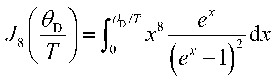
| This journal is © The Royal Society of Chemistry 2021 |