Tools and methods for circular dichroism spectroscopy of proteins: a tutorial review

Abstract

Circular dichroism (CD) spectroscopy is a widely-used method in biochemistry, structural biology and pharmaceutical chemistry. More than 24 000 papers published in the past decade have included CD characterisations of proteins; many of those studies have also included other complementary chemical, biophysical, and computational chemistry methods. This tutorial review describes the background to the technique of CD spectroscopy and good practice methods for high quality data collection. It specifically focuses on both established and new methods and tools available for experimental design and interpretation, data processing, visualisation, analysis, validation, archiving, and accession, including tools developed to enhance the complementarity of this method with other structural and chemical biology studies.

---

A. J. Miles

Andrew Miles obtained a first class degree in Biological Chemistry at the University of Leicester, a masters in Biotechnology from Liverpool John Moores University, and in 2005, a PhD in Structural Biology in Professor Wallace's lab at Birkbeck College, where he is now the senior postdoc in the circular dichroism group. He has also recently gained a first class degree in Physics from the Open University. He is involved in methods development and spends much of his time collecting data at SRCD beamlines in Denmark, France and Germany.

Robert W. Janes

Robert W. Janes is a Senior Lecturer in the School of Biological and Chemical Sciences, at Queen Mary University of London. He obtained his BSc in Chemistry at Royal Holloway College, University of London, and his MSc and PhD in Crystallography at Birkbeck, where he later undertook his postdoctoral work. His current work focuses on tools and resources development for circular dichroism and synchrotron radiation circular dichroism spectroscopies, and creation of other bioinformatics tools for studying proteins. He is co-director (with BAW) of the Protein Circular Dichroism Data Bank.

B. A. Wallace

Bonnie Ann Wallace is Professor of Molecular Biophysics in the Department of Biological Sciences at Birkbeck, University of London and at the UCL/Birkbeck Institute of Structural and Molecular Biology. She obtained her PhD in Molecular Biophysics and Biochemistry from Yale, was a Jane Coffin Childs postdoctoral fellow at Harvard and at the MRC Lab of Molecular Biology, Cambridge, an Associate Professor of Biochemistry at Columbia University, and Professor of Chemistry/Director of the Centre for Biophysics at Rensselaer Polytechnic Institute. In 2020 she received the Royal Society of Chemistry Khorana Prize for her work on membrane protein structures and methods.

---

Key learning points

1. Circular dichoism (CD) spectroscopy, a widely-used method for examining the structures and conformational changes of proteins, provides complementary information to that obtainable by other biophysical, chemical, and structural biology techniques.

2. Methods for good practice in measuring, processing, analysing, and interpreting CD spectra of proteins are described.

3. Means of accessing and utilising links to a wide range of online and downloadable tools for comparisons, secondary structure analyses, and predictions of CD spectra are presented.

4. Information is provided on how to access archived CD data sets and associated metadata in the Protein Circular Dichroism Data Bank (PCDDB), and its links to other data bases and validation protocols, and online information.

5. Examples of recent studies and developments utilising CD in novel studies of proteins exemplify its complementarity to other methods.

1. Introduction to circular dichroism spectroscopy of proteins

Biomolecules such as proteins are built up of chiral subunits that produce signals when illuminated by circularly-polarised light in the near and far ultraviolet wavelength ranges where the amide and carbonyl groups of the polypeptide backbones absorb. Circular dichroism (CD) spectroscopy is an optical spectroscopic method which exploits the differential absorption of left- and right-circularly polarised light by such chromophores, and can be harnessed to derive structural information about protein conformations. It has been widely used to discern the secondary structure of proteins based on electronic transitions in the far ultraviolet (UV) wavelength region (∼240 to 170 nm) and to monitor the local tertiary structure environment of aromatic amino acid residues in the near UV region (∼300 to 260 nm), as a function of their physical or chemical environment, amino acid composition (i.e. mutations), or intermolecular interactions.^1–4 In the past decade, more than 24 000 papers have been published using CD spectroscopy to characterise the structures of polypeptides and proteins. The information derived by CD spectroscopy, which can also include information on dynamic changes in solution or in environments such as membranes or films, is often complementary to that produced by other biophysical, computational and chemical methods such as crystallography, cryo-electron microscopy, NMR spectroscopy, FTIR spectroscopy, vibrational circular dichroism (VCD) spectroscopy,⁵ molecular dynamics simulations, and low angle scattering. Indeed, in the same 10 year time period, nearly half of the publications which included CD spectroscopy also included information derived from at least one of these other techniques.

CD spectroscopy has a number of advantages with respect to the higher resolution structural techniques such as crystallography, electron microscopy, and NMR spectroscopy in that it requires relatively small amounts of sample under conditions (temperature, concentration and components present) that may be more comparable to those found in cells. This has resulted in its wide-spread use both by the biochemical and structural biology communities to complement the information derived by those other biophysical methods,⁴ as well as by the pharmaceutical industry,^6,7 to assess whether a protein is correctly folded, to monitor structural changes induced by interactions with ligands including other proteins, and to determine protein stability under environmental stresses induced by, for example, changes in pH or temperature. In recent years circular dichroism beamlines have been developed at synchrotron light sources, taking advantage of both their high light flux, which enables faster collection of data from smaller amounts of protein, and the higher information content available due to the lower wavelengths that can be achieved at these high-intensity light sources.⁸

This tutorial review discusses not only methods and software currently available for obtaining, processing, validating, and interpreting high quality CD data obtained using lab-based (commercial) CD instruments (as well as synchrotron radiation circular dichroism (SRCD) beamlines) on a variety of samples types, but also the bioinformatics tools and resources available for determining novel details of the structure and function of proteins based on such data.

2. Methods, tools, and protocols for CD data collection, analyses, and display

2.1 Measuring CD spectra

To optimise the amount of high quality and reproducible CD data obtained from a given sample, it is essential to follow good practice protocols for data collection (see Table 1 for example).^8,9 To accurately determine the secondary structure of a protein based on CD data, the data obtained must include a spectral range covering, at least, the wavelengths between 240 and 190 nm; more accurate results are obtained if data collected includes even lower wavelengths, because more electronic transitions (peaks) will be included, increasing the information content of the data. To achieve such measurements, conditions must be used so that the total absorbance of the sample (due to protein, buffer and other added components) is below ∼1.2 at all wavelengths. This may be challenging for wavelengths below 210 nm, where the absorbance tends to rise, sometimes precipitously, due to the cumulative effects of the buffer and the peptide chromophores along with contributions from water (or other solvents) and the composition material of the optical cell. In addition, light scattering effects from any undissolved protein or suspended particles in the solution, such as lipids present in membrane samples,⁹ may also contribute to this challenge.

Table 1 Workflow for recommended data collection and processing procedures. The column on the right indicates how to avoid potential problems that may arise

Procedure	Notes
Prepare highly purified protein in low absorbing buffer	≥95% of protein should be the protein of interest
Based on estimated concentration choose a cell pathlength so that the absorption is <1.2 at all wavelengths	If the absorbance is too high, choose a shorter pathlength cell or a different buffer
Verify cell pathlength	Cells with pathlengths <0.1 mm can be measured using the interference fringe method
Measure protein concentration accurately	If possible, measure concentration again immediately before measuring spectrum
Collect repeat CD spectra of sample and baseline	Monitor the HT signal. Make sure it does not exceed the linear range of the instrument
Average the sample data	Make sure there are no outliers due to un-equilibrated or leaking or light-sensitive sample or buffer components
Average the baseline data
Subtract averaged baseline from averaged sample	Make sure the baseline and sample spectra overlay at wavelengths >250 nm (where there should not be a protein signal)
Calibrate the net (sample-baseline) spectrum (optional)	Important when comparing spectra measured on different instruments or after the lamp has been changed
Scale to standard units	Using the determined values of cell pathlength, protein concentration and mean residue weight

---

The overall absorbance of the sample can be monitored by the dynode voltage or high tension (HT) signal produced during data collection. This is a measure of the voltage applied to the detector to amplify the small circular dichroism signal. The maximum HT cutoff values for individual CD instruments differ, but they correspond to the maximum dynode voltage reading above which the sample absorbance is too high for sufficient light to penetrate. Above this value the apparent CD signal and the intensity of the unpolarised light signal that emerges from the sample decrease to a level where the spectrum becomes noisy, and lead to distortions in both the magnitude and the shape of the measured peaks. Hence the maximum HT value for a given CD instrument needs to be determined.

For a given sample, minimisation of the total absorbance can be achieved by choosing buffer constituents with low absorbance in both the near and far UV wavelength region, and where this is not possible, using the lowest possible concentration of buffer and salts without compromising the stability of the protein. In addition a combination of protein and buffer concentrations, optical cell pathlength, optical cell material, and instrument parameters such as slit width and averaging time can be used to optimise the CD signal.^8–10

Secondary structure analyses are also significantly affected by the accuracy of the protein concentration measurement, since this will have an effect on the magnitude of the CD spectrum when scaled to standard units.^8,9 The most widely used colorimetric methods for determining protein concentrations, including Biuret, Lowry, bicinchoninic acid assays, and Coomassie blue staining; all produce different values/accuracies for proteins (depending on their amino acid compositions). Measuring the absorption of the sample at 280 nm (A₂₈₀) is the most convenient and reliable method (although its accuracy can depend on the number of aromatic amino acids and to a lesser extent, their location (surface or buried) in the protein). Such measurements can be achieved (without wasting a great deal material) using micro-UV spectrometers such as Nanodrops.

Another important consideration is if there is a time lag between sample preparation, concentration determination, and CD measurements, or even during the course of a long series of CD measurements, there may be a change in the protein concentration, due to aggregation or precipitation, especially if the sample is unstable or sensitive to light. This issue can be obviated in part by measuring the concentration of the protein immediately before (or as near in time as possible to) measuring the CD spectrum. It can also be monitored by examining the HT measurements obtained during the course of the CD measurements. If the HT values decrease, this could be indicative of protein precipitation/aggregation, bubble formation, or even sample leakage, during the course of the measurement, and should indicate that a new sample needs to be used.

Using an inaccurate value for the optical cell pathlength will also have significant effects on spectral magnitude and therefore the accuracy of secondary structure analysis. This can be an issue when using demountable cells with pathlengths less 0.01 cm, as the manufacturer-reported values can have a wide margin of error. In addition, the loading and assembly of such cells can be non-reproducible.¹⁰ However, accurate pathlength measurements can be obtained for these cells using the interference fringe method,¹⁰ which requires use of a standard benchtop UV/Vis spectrophotometer.

Finally, as CD instruments are comprised of a number of optical components, there can be variations between instruments which lead to small differences in spectra of the same sample measured on two different instruments. Such disparities can be reduced or mitigated by obtaining calibration measurements with a standard reference material such camphorsulphonic acid (CSA) or ammonium camphour sulfonate (ACS) measured on the same instrument used for the sample measurements.^7,11,12 Both of these compounds have two well-defined and well-separated peaks of known absolute magnitude, so comparisons between the calculated and the experimental values can be used to create a calibration curve over the wavelength range of the spectrum. Multiplying the measured CD values of the protein spectrum by the CD values of this curve at each wavelength, will adjust the spectrum so that it better matches the spectra measured on any other instrument where this procedure is carried out.

2.2 Processing methods and tools

CD spectra are usually produced by averaging a set of repeat scans (or accumulations) obtained for the sample, after which the averaged spectrum of the baseline (a solution that contains all components of the sample except the protein), is subtracted. The final net spectrum can then be calibrated against a solution (CSA or ACS) with a known signal, and normalised to standard units of mean residue ellipticity (MRE, degrees cm² dmol⁻¹ residue⁻¹) or delta epsilon (Δε, M⁻¹ cm⁻¹) using the concentration, optical cell pathlength, and mean residue weight value for the protein. Each step in this process provides an opportunity to identify anomalies in the data. For example, there may be a systematic change in the data as a function of time that is apparent in repeated scans (possibly as a result of light-inducted conformational changes, or because the protein precipitates/aggregates with time). Processing data using a standard spreadsheet is possible but this method can be time-consuming; hence there are a number of possible alternatives described in this section.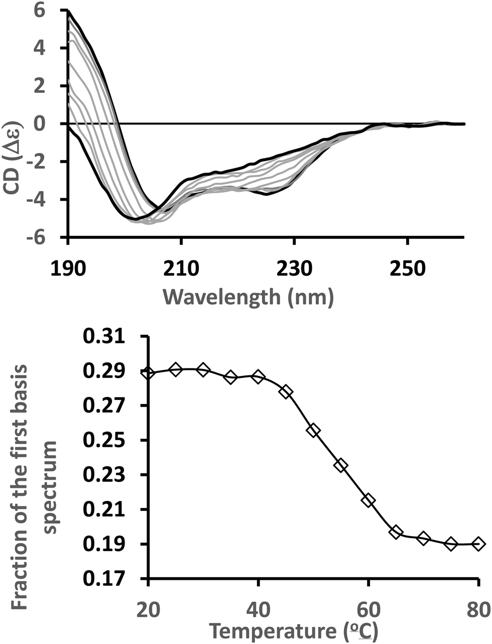

2.2.1 Instrument-associated software. CD instruments are supplied with their own data processing software packages, which enable basic processing procedures such as averaging of scans (accumulations), baseline subtraction, scaling to standard units and data smoothing. These functions are found in the “spectra manager” for Jasco instruments and the “trace manipulation menu” in the Pro Data viewer provided with the Chirascan spectrophotometer. For both the Aviv and Olis instruments, they are in the data processing menu. All manufacturers also provide a comprehensive set of mathematical functions, ranging from simple arithmetic such as scaling and normalisation at a peak wavelength to curve fitting. The Olis software also includes software for basic dataset analyses using Singular Value Decomposition (SVD) methodology, also available in CDtool software. This is a form of principal component analysis for a set of spectra, for example from a temperature or time series, in which the spectral features are reduced to a small number of principal components or basis spectra that, in different proportions, can be summed to reproduce each experimental spectrum in the series. The coefficients that determine the contribution of a particular basis spectrum can be plotted as a curve that represents the change in secondary structure during the course of the experiment. SVD analyses provide alternatives to monitoring the CD signal at a single peak wavelength to identify changes, and have the advantage of incorporating information from the entire wavelength range of the spectrum rather from just a single wavelength (see Fig. 1).

Fig. 1 Singular value deconvolution analysis of a set of spectra from a thermal melt series. Top: Spectra of alpha-lactalbumin (PDB 1A4V) measured at temperatures ranging from 20 °C to 80 °C in 5 °C steps. Bottom: Fraction of the first basis spectrum at each temperature following SVD analysis.

Instrument-processed data can be exported in ASCII format for external use including secondary structure analysis using the tools described in Section 3. However there is no consensus of file structure which would enable comparisons of data produced on different instruments, for example, data collected on a benchtop instrument and at an SRCD beamline, or two different bench-top instruments, which would enable simple comparisons. For this reason, the generic data processing software CDToolX,¹³ which is described in the following section, was created for use with the output of any CD or synchrotron radiation circular dichroism (SRCD) instrument, and provides formatted output results that are instrument-independent.

2.2.2 CDToolX. CDToolX,¹³ and its predecessor CDtool,¹⁴ are freely-available, downloadable tools designed for data processing and for some types of analyses of protein CD spectra. CDToolX¹³ is designed for use on Windows 10 operating systems (or with Windows 10 emulators on other operating systems), whereas CDTool¹⁴ works on earlier operating systems such as Windows 7 and Windows XP (which may often be installed on older CD instruments) or Mac-based Windows emulators. At present, CDToolX¹³ is compatible with files created by the following instruments (and possibly others): Aviv, Jasco, (.txt file outputs only), Applied Photophysics, Chirascan (.cdnn format), and outputs by most SRCD beamlines. In addition, an ASCII text file with two tab-delimited columns containing wavelength and CD data (i.e. those generated by spreadsheets), and generic files (.gen) produced by the original CDTool¹⁴ program can be used. This software was specifically designed to enable identification of data anomalies before they are incorporated into the final processed spectrum, a strategy that provides a complete data trail for archiving and regulatory purposes. Additionally, cross instrument comparison can be enhanced by calibration performed using spectra of CSA or ACS, which adjusts for differences in instrument polarisation. The simple math operations supported include smoothing, spectral magnitude scaling and scaling of multiple spectra to each other at selected wavelengths as a sensitive means of detecting spectral differences in cases where the concentrations of the protein in the samples has not/cannot be accurately measured (Fig. 2). SVD of datasets can also be performed (Fig. 1) and the data can be stored in a local MySQL database to be retrieved in the CDToolX¹³ plot window in units of Δε or mdeg, either calibrated or uncalibrated.

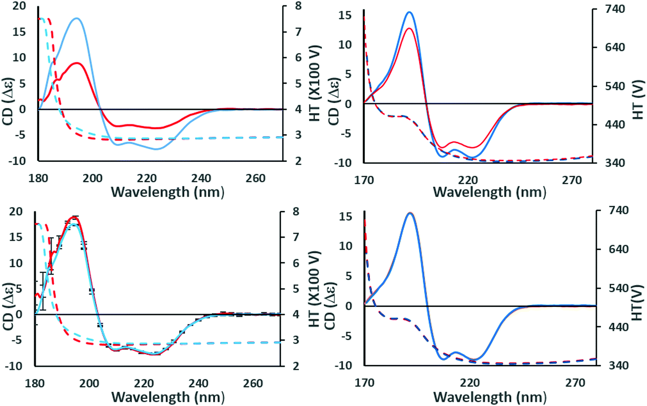Fig. 2 Example of identifying the effects of scaling errors during data processing. These panels show the effects of scaling a spectrum at a single wavelength to check for similarities and correct for magnitude errors. (top left) The (incorrectly scaled) spectra of wild type (red) and a mutant (blue) construct of the NavMs voltage-gated-sodium channel (PDBID 5HDX). There are large differences in the magnitudes of the CD spectra (solid lines) although their shapes are similar. This could be due to a magnitude/scaling error resulting from the use of inaccurate concentration or pathlength values in the calculations, but it can be checked as follows: (bottom left) the CD spectra are scaled to the same CD value at the 222 nm peak, making it evident that there is a small but significant difference between their spectral shapes (and note the small vertical reproducibility bars at 5 nm intervals do not overlap at the peak ∼195 nm, although they do overlap at the high wavelength peaks). However, the protein structures are not the same, and the difference due to the mutation can be quantified. Since neither of the corresponding high tension (HT) spectra, which is a measure of sample absorbance (dotted lines, same panels, with scale on right hand side of the plot), have exceeded the (predetermined) instrument cutoff value of 5 at wavelengths below ∼190 nm, this also confirms there has been no distortion of the peak due to too high absorbance. (top right) Spectra of calmodulin (PDBID 1LIN) at different pH values. In this case there is also a significant difference in the magnitudes of the CD spectra; however, scaling to the same values at 222 nm (bottom right) indicates that, in this case, because the scaled spectra overlay at all wavelengths, the apparent difference was due solely to concentration or pathlength measurement errors.

2.2.3 Summary. Instrument manufacturers provide a comprehensive set of instrument-specific tools for processing, analysis and data manipulation, whereas CDTool¹⁴ and CDToolX¹³ are dedicated to the basic tasks required by a majority of users. The latter also provide a transparent user-friendly environment, which enables comparisons of data between instruments, and facilitates CSA calibration to adjust for differences in instrument polarisation. Furthermore CDToolX¹³ is the primary processing software used at a number of SRCD beamlines around the world.

2.3 Methods and tools for analysing protein secondary structure from CD data

Protein CD spectra include two types of electronic transitions arising from peptide absorptions in the far UV.¹ These include an n → π* transition that gives rise to a signal at ∼222 nm, and parallel and perpendicular π → π* transitions that give rise to signals at lower wavelengths in the range from ∼190–210 nm (illustrated in Fig. 3). In addition, an intra-amide charge transfer transition arising from through-space interactions occurs at around 180 nm, which is generally only accessible using synchrotron radiation as a light source.⁸ The different types of secondary structures that are adopted by polypeptide chains (for example, helix or beta strand) depend on the dihedral (Φ, Ψ) angles between adjacent residues in the polypeptide chain; the magnitudes and wavelengths of the CD signals that arise from the electronic transitions depend upon these angles and therefore upon the secondary structure of the protein. The overall shape and magnitude of a protein CD spectrum in the far ultraviolet (UV) wavelength region reflects a linear combination of its constituent secondary structural elements. Fig. 4 shows examples of spectra of proteins that are each dominated by one type of secondary structure, but most proteins contain multiple types of secondary structures that all contribute to their net CD spectrum.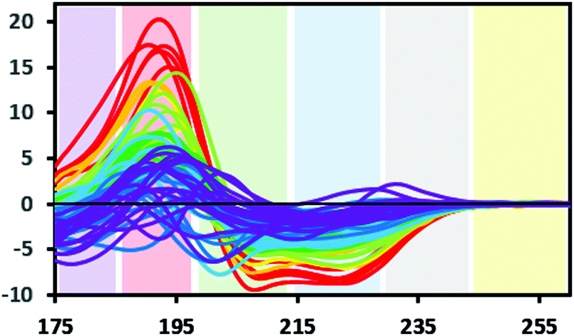

Fig. 3 Bands defining the approximate wavelength range for electronic transitions responsible for the CD signals: Yellow: Signals due to aromatic residues (if present) may be detected in 100× pathlength cells; grey: occasionally a signal may be detected here due to the presence of stacked aromatic amino acids,¹ blue: n → π* transition. Green and red: π → π* transition, this transition can give rise to two peaks due to exciton splitting, purple: charge transfer transition (generally only detectable when using synchrotron radiation source) (SRCD spectra). The depicted spectra are from the SP175 dataset²¹ and are available in the PCDDB³⁵ with codes CD0000010000 to CD0000710000. They are shaded according to percentage of helix in the crystal structure of the protein as follows: red: 70% +, orange: 60–70%, yellow: 50–60%, light green: 40–50%, dark green: 30–40%, light blue: 20–30%, dark blue: 10–20%, purple: 0–10%.

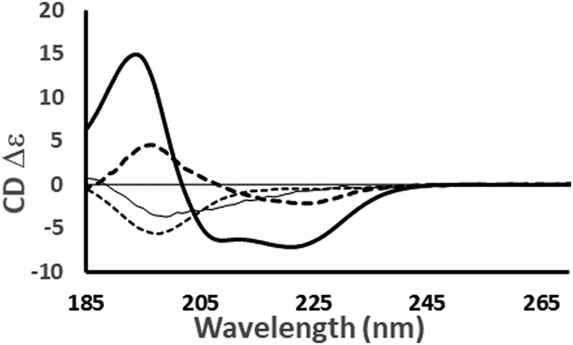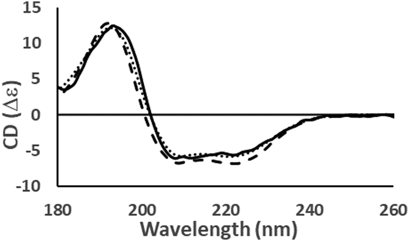
Fig. 4 Examples of the different shapes and magnitudes of CD spectra of proteins comprised primarily of different types of secondary structure: Predominantly helical [haemoglobin] (); predominantly anti-parallel beta sheet [concanavalin A] (- - -); predominantly right-hand twisted beta sheet [elastase] (—); predominantly disordered [HASPA] (⋯). The spectral data used in this figures are available in the PCDDB³⁵ with accession codes: CD0000037000, CD0000020000, CD0000031000 and CD0005282000, respectively. The shape and intensity of each spectrum arises from the sum of all the secondary structure elements present in the protein (Fig. 3). There is no single band attributable to a certain secondary structure element, however, in general the magnitude of a negative peak at ∼222 nm is dependent on alpha helical content whereas a negative peak at ∼200 nm is indicative of disorder.

There are a number of deconvolution methods available for obtaining quantitative secondary structural information from CD spectra,^1,2,14 each of which requires a reference dataset of CD spectra produced from proteins with known (crystal) structures, in order to produce a calculated secondary structure spectrum that best matches the query (experimental) spectrum. These methods range from relatively simple least squares algorithms, to more complex ridge regression (RR) and singular value deconvolution (SVD) methods with variable selection (VS) functions, which fit the experimental spectrum to a weighted sum of the individual reference spectra. In general, a broader-base (more, and more varied) of components present in the reference database, allows more accurate identification of the protein structure that produced the query spectrum. However, the results of some types of analyses can be optimised by the use of specialised datasets, such as those designed for integral membrane proteins (which, due to their presence in low dielectric environments, tend to have transitions at somewhat different wavelengths than soluble proteins^2,11). The characteristics and component types of current publically-available datasets are listed in Table 2, along with an indication as to which type of protein each database is best suited for.

Table 2 Characteristics of currently-available reference datasets for use in CD analyses, and the servers on which they are available. The final column indicates the types of proteins for which the dataset may be best suited. The individual protein spectral data comprising the SP175²¹ and SMP180²² datasets can be downloaded from the PCDDB³⁵

Reference dataset	Wavelength range (nm)	Number of proteins	Server	Types of proteins
SET1^25	178–260	29	DichroWeb^16	soluble, globular
SET2^25	178–260	22	DichroWeb	soluble, globular
SET3^25	185–240	37	DichroWeb	soluble, globular
SET4^25	190–240	43	DichroWeb	soluble, globular
SET5^25	178–260	17	DichroWeb	soluble, globular
SET6^25	185–240	42	DichroWeb	soluble, globular and denatured proteins
SET7^25	190–240	48	DichroWeb	soluble, globular and denatured proteins
SP175^21	175–240	71	DichroWeb	soluble, globular (bioinformatics definitions)
SMP180^22	180–240	129	DichroWeb	membrane and soluble proteins
SP175+^29	175–240	79	BeStSel^29	soluble, globular especially β-sheet

---

Alternative analysis methods¹⁵ use neural networks (NN) trained on sets of CD reference data. The accuracy of these depend upon both the suitability of the dataset used for training, on the breadth of protein spectra available, and the spectral wavelength range covered.

2.3.1 The DichroWeb analysis server¹⁶. DichroWeb is a freely-available online resource for determining protein secondary structures based on CD and SRCD spectra. It provides five different calculation algorithms [CONTINLL¹⁷ (a regression restraint method), SELCON3,¹⁸ CDSSTR¹⁹ and VARSLEC²⁰ (all SVD methods with variable selection), and K2D¹⁵ (a neural network method now superseded by the stand-alone K2D3 method – see Section 2.3.3)]. These methods can be used with the reference datasets noted above, except for K2D, which uses its own reference data, and VARSLEC which has a built-in (unchangeable) dataset.

The dataset chosen for use will depend on the type of protein to be analysed. For example, to analyse the spectrum of a highly structured soluble protein, an appropriate choice may be SP175,²¹ which contains 71 high quality spectra of a bioinformatics-defined set of soluble globular proteins, covering all protein fold classes, which has a selectable wavelength range covering 175 nm to 240 nm. Alternatively, the SMP180²² dataset contains not only spectra of the soluble globular SP175²¹ proteins, but also 29 membrane protein spectra with low wavelength cutoffs of 180 nm, and hence is more suitable for analysing membrane proteins. The choice of dataset may be restricted by the low wavelength cutoff of the experimental data: for data which extend to a low wavelength of only 190 nm, truncated versions of SP175²¹ and SMP180²² are available. Spectral data that do not extend to wavelengths at least as low as 190 nm or below are not suitable for analysis by DichroWeb,¹⁶ as they do not have sufficient information content to enable detailed definitions of secondary structure.²¹ The secondary structure definitions used to create these reference datasets are those defined by the “Dictionary of Protein Secondary Structures” (DSSP) algorithm,²³ based on conformational characteristics identified in crystal structures.

The DichroWeb¹⁶ server accepts file formats produced by most commercial and SRCD instruments, plus CDToolX¹³- and CDTool¹⁴-generated files, and simple two column (wavelength, value) text files. User files can be directly uploaded to the online server, and a number of parameters can be manually selected, including the high and low wavelengths of the data, the lowest wavelength to be considered in the analysis (which may differ from the lowest wavelength collected, if that wavelength resulted in an HT value that exceeded the cutoff limit of the instrument), and the spectral units, either mdeg or mean residue ellipticity (MRE). Input of the wavelength step size is also required. The algorithm and dataset to be used are selected from a dropdown box, and if the input spectrum has units of mdeg, the concentration in mg ml⁻¹, optical pathlength in cm, and the protein mean residue weight are also required inputs so that the spectrum can be converted to MRE units prior to analysis.

The output pages (Fig. 5a and b) provide both a compact and an extended listing of the secondary structural results, and a plot of the back-calculated spectrum based on the secondary structure determined, which is overlaid on the experimental spectrum, as a visual indicator of the quality of the result (i.e. correspondence between the shapes and magnitudes of the calculated and measured spectra). The compact results table simply lists the predicted secondary structure fractions, whereas the extended results table (Fig. 5a) also provides a goodness-of-fit parameter known as the normalised root mean squared deviation (NRMSD²⁴) which is an indication of the correspondence between the measured data and the back-calculated spectrum produced from the derived secondary structures, and is similar to an “R-factor” in crystallography. It is defined as:

where θ_exp and θ_cal are the experimental and back-calculated ellipticities, respectively, at each wavelength in the spectrum. Analyses that produce high NRMSD²⁴ values (>0.1) or poor correspondences between the experimental and calculated best fit spectra are strong indications that the protein of interest includes features not present in any of the proteins present in the reference data base.

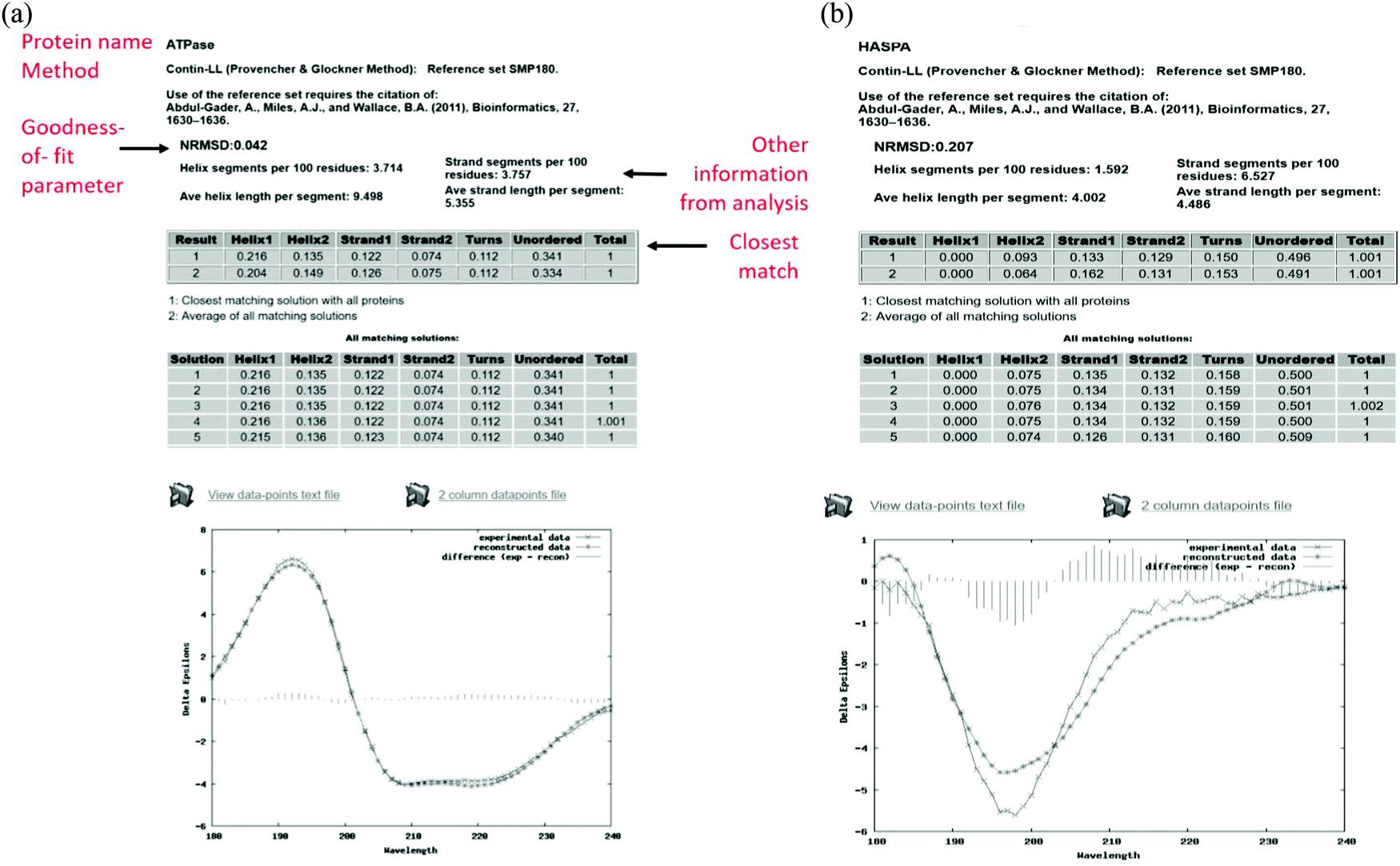Fig. 5 (a) Example results page obtained using the DichroWeb¹⁶ server for a “good quality analysis”. (top) The protein name (ATPase, PCDDB³⁵ code (CD0004003000)) is displayed and the analysis method used [ContinLL¹⁵] is listed on the next line. Below this is the NRMSD²⁴ “goodness-of-fit parameter”, which should optimally be <0.1 (as it is in this example), indicating a close correspondence between the back-calculated and measured spectra. If it is not, then another method, reference data set and/or scale factor should be used. (middle) Tables [shaded areas] of calculated secondary structure results obtained using the CONTINLL¹⁷ method and the appropriate (SMP180,²² membrane protein) reference data set. The arrow at the right of the top row indicates what is usually the closest/most suitable solution. The lower shaded box indicates other possible solutions obtained using other types of calculations. (bottom) Plot showing a comparison of the experimental spectrum (crosses), the back-calculated closest match spectrum (stars), and the difference spectrum (vertical bars) between the experimental and back-calculated spectra (vertical lines). The low NRMSD²⁴ is consistent with the close match of the calculated and experimental spectra. These, plus the small magnitude difference spectrum indicate this is a “good quality” analysis. (b) Example results page obtained using the DichroWeb¹⁷ server for a “poor” quality analysis. This was obtained for an intrinsically disordered protein, HASPA (PCDDB code: CD0005282000). As in Fig. 5a, except in this case neither the (high) NRMSD²⁷ value (>0.1) nor the correspondence between the calculated and experimental spectra, suggest that the best solution is an accurate reflection of the secondary structure. This is because this is an intrinsically disordered protein and is comprised of mostly unordered or disordered (not helical, sheet nor turn) secondary structures. As such it does not have well-defined phi, psi angles, and as the reference dataset does not contain many spectra of proteins with significant amounts of disorder (largely because this type of protein does not tend to crystallise), the NRMSD²⁷ value is high. There is also a greater difference between the experimental and back-calculated spectra for this protein as compared to that for the well-ordered protein depicted in the Fig. 5a.

The calculated results (Fig. 5) include the following secondary structure types: regular and distorted alpha helix, regular and distorted beta sheet, and turns.²⁵ The distorted helix and sheet fractions include the residues at either end of an alpha helix and one residue at either end of a beta strand, which have slightly different dihedral angles than the corresponding canonical structures based on crystallographic data and thus have slightly different characteristic spectra. The ‘turn’ fraction includes beta turns, bends, and bridges as defined by DSSP.²³ All other types of structure, including random coil, are classified as ‘unordered’. Two exceptions to these classifications are those produced by dataset 2, which uses as structural assignments α-helix, 3₁₀ helix, β-strand, turn, polyproline-II helix, unordered, and dataset 6 which uses the same structural definitions but combines the two types of helical fractions.^26,27

The predicted average helix and strand lengths (which may or may not be accurate depending on the protein structural type, and hence should not be relied upon), and a list of solutions to all iterations of the calculations as the algorithm approaches the best fit back-calculated spectrum solution are also listed.

A further calculation option is that of a variable scale factor, which enables the user to multiply the input data by a small factor (<±0.1) to compensate for small experimental spectral magnitude errors²⁸ (as illustrated in an example for the protein hemerythrin in Table 3a).

Table 3 (a) Examples of secondary structure percentages calculated using different methods of analyses and different reference datasets for soluble proteins, compared with the values obtained from their crystal structures. For this comparison, all spectra were analysed in the wavelength range from 240 nm to 190 nm, and only the percentages of total helix and total sheet are indicated. The last two rows (for hemerythrin) demonstrate the effect of spectral magnitude (scaling factor of 1.0 (penultimate line) vs. 1.3 (final line)) on the NRMSD²⁴ goodness-of-fit parameter (column 1), and the calculated secondary structures (columns 3–6). For the correct scaling (1.3 in this case), the resulting NRMSD²⁴ is smaller than that for the incorrectly scaled data, and the calculated structure more closely matches secondary structure of the protein, as calculated from the crystal structure (column 7) using DSSP²³ (b) Example of secondary structure analyses for a mostly disordered protein (the hydrophilic acylated surface protein (HASPA) from L. major) using different calculation methods and reference data bases. As is typical for intrinsically disordered proteins, there is no crystal structure available for it, so the values given in the last column are average values calculated from several bioinformatics prediction sites (SPOT-1D, RaptorX, NetSurfP). “Other” indicates disordered secondary structure (i.e. neither helix nor sheet). Its spectrum (Fig. 3) clearly indicates (from its shape) that the protein is mostly disordered; however since there are no fully-disordered proteins in the PDB³⁰ and hence in the CD reference datasets, even the “best” results produced a relatively poor (high) NRMSD²⁴ values, and only modest matches to the bioinformatics predictions

(a)
Protein name (PDB ID) or PCDDB ID	Secondary structure	% Secondary structure calculated using				% Secondary structures from crystal structure
		Server
		METHOD
		Dataset
		DichroWeb^16	DichroWeb	BestSel^29	K2D3^32
		CONTINLL^17	SELCON3^17	SP175+^29
		SP175t^21	SP175t
Caletexin	Helix	58	63	61	53	62
CD0004676000	Sheet	5	5	0	10	2
Antithrombin	Helix	27	29	32	23	26
CD0003889000	Sheet	26	22	18	25	27
Bj-xtrIT	Helix	27	28	25	15	26
CD0004244000	Sheet	20	8	20	21	18
Hemerythrin	Helix	53	54	50	50	70
(1HRT), scale1.0	Sheet	15	15	7	11	0
NRMSD = 0.055
Hemerythrin	Helix	67	69	75	66	70
NRMSD = 0.029	Sheet	7	4	7	2	0
(1HRT), scale1.3

---

(b)
Protein name PCDDB ID	Secondary structure	% Secondary structure calculated using						Average % from Bioinformatics
		Server
		METHOD
		Dataset
		DichroWeb^16	DichroWeb	DichroWeb	DichroWeb	BestSel^29	K2D3^2
		CONTINLL^17	SELCON3^17	CONTINLL	SELCON3	SP175+^29
		SP175t^21	SP175t^21	SET6^25	SET6^25
HASPA	Helix	9	14	4	6	0	2	4
CD0005282000	Sheet	30	27	15	13	34	23	1
	Other	61	59	81	81	66	75	97
	NRMSD	0.104	0.399	0.145	0.214	0.015	—	—

---

2.3.2 The BeStSel server²⁹. BeStSel is a secondary structure analysis server (Fig. 6) that was specifically designed for the analysis of beta sheet-rich proteins, although it can be used for any class of (soluble) protein. It employs a selection method algorithm based on SVD and an enhanced version of the SP175²¹ dataset (designated SP175+) which contains extra beta-sheet reference spectra, covering regions of fold space not present in the SP175²¹ dataset. This enables it to better resolve parallel and antiparallel sheet components, with a further division of the latter into left-hand twisted, relaxed, and right-hand twisted sheets. It also provides predictions of fold motifs for beta-sheet rich proteins corresponding to the topology level organisation in the CATH protein fold database,³¹ and is based on a match of the calculated secondary structure of proteins with similar DSSP²³ values as found in the Protein Data Bank (PDB);³⁰ however, it is important to note that these folds may or may not actually correspond the structural fold type found in the test protein. As in DichroWeb,¹⁶ the spectral magnitude can be scaled by a chosen amount to identify the prediction with the lowest NRMSD,²⁴ or the ‘best factor’ function can be selected, which automatically scales the spectra by factors between 0.5 and 2.0.

Fig. 6 Workflow for analyses using the BeStSel server.²⁹ (1) The initial secondary structure analysis displays the input spectrum and back-calculated spectrum, along with the predicted secondary structure fractions (displayed both as a table and a pie chart). (2) The experimental spectrum is rescaled by a user-defined factor and reanalysed, or (3) the spectrum is automatically scaled using the “best factor” function. The results of the latter provide a graph of the NRMSD value²⁴ (same definition as in the DichroWeb¹⁶ server) as a function of scale factor, along with the associated values for the calculated secondary structure fractions. (4) Ribbon diagrams for proteins with similar secondary structure compositions (but not necessarily the same folds) as the proteins.

2.3.3 The K2D3 server³². The K2D3 server, a successor to the K2D method (which is still included in DichroWeb¹⁶), is a neural network-based method trained on a dataset of theoretical CD spectra produced using the DichroCalc³³ server (see Section 2.7.1), and uses a non-redundant selection of folds represented in the PDB.³⁰ The predicted spectrum is constructed from the most similar CD spectra in this set, weighted by their distances from the query CD spectrum (provided in either Δε or MRE units). There is an option to include the protein molecular weight in kilodaltons, or the number of amino acids in the polypeptide. The output includes the query spectrum overlaid on the back-calculated spectrum, plus the predicted percentages of helix and strand. There is no measure of the quality of the fit, although a warning is displayed if the distance between the query and the most similar spectrum in the dataset is larger than a threshold value.

2.3.4 Summary comparison of analysis methods and reference data sets. The analysis programs described above offer options that include a range of methods and reference datasets and, for globular soluble proteins, they tend to give very similar results, especially for proteins with high helix contents (Table 3a). Analyses of beta sheet-rich proteins tend to vary more between methods because of the wide range of secondary and tertiary structural features present in proteins containing these types of features; analyses of β-sheet proteins appear to be a strength of the BestSel²⁹ method, which takes some of these variations into account.

Currently the SMP180 dataset²² available in DichroWeb¹⁶ is the only bespoke reference dataset available for analysing membrane proteins, which tend to exhibit peaks at slightly different wavelengths than soluble proteins with the same secondary structure content. Use of this reference data set may improve predictions for membrane proteins.

Despite the wide range of secondary structure analysis methods and dataset options, characterisations of proteins with high fractions of disordered structure are still challenging. Such proteins tend not to crystallise, so in the PDB³⁰ there are relatively few crystal structures which are not primarily composed of canonical secondary structure types, although individual entries may include some disordered regions. As a result, all the analysis methods that rely upon reference to known protein structural types are less successful in defining the structures of such proteins, which are generally referred to as “intrinsically-disordered proteins”. Such spectra can often be identified visually as they tend to display only a single negative peak at ∼200 nm (Fig. 4 and 5b), and can sometimes resemble the spectra of some beta-rich proteins in both shape and magnitude (but with an altered peak position). Consequently, analyses using any of the existing datasets often assign significant amounts of beta structure to these spectra (Fig. 5b and Table 3b). Only datasets 6 and 7 in DichroWeb¹⁶ contain the spectra of any denatured proteins (which may or may not be similar to disordered proteins), but as disorder covers a wide range of (often flexible) secondary structural features, none of the presently available analyses are particularly suitable for this important class of proteins. Unfortunately, such proteins or regions of proteins appear to play important roles in the regulation of cell functions, and are also not well characterised by other (complementary) structural methods such crystallography, NMR and IR spectroscopies.

2.4 Identifying spectral artifacts and improving CD spectra

Quality control considerations for both the integrity of proteins under study and the analysis methods used to characterise them are important for producing suitable CD analyses. This has led to the development of ValiDichro³⁴ software that can be used to identify some artifacts and irreproducibility in CD data, and/or errors in the parameters used for calculating secondary structures from CD data.

2.4.1 The ValiDichro server³⁴. The ValiDichro server³⁴ provides a means of testing CD data and associated metadata as a guide to good practice and to aid publication. As well as the dedicated standalone server, there is a version embedded in the PCDDB,³⁵ which is used to vet depositions before they are included as entries in the database. Data quality tests are based on the common characteristics of CD protein spectra observed in the literature and are given a designation of a pass (P), a flag (F) for small deviations from the norm, or a fail (X) if the deviation is more severe.

ValiDichro³⁴ tests CD spectral data quality, reproducibility, and completeness (wavelength range), as well as the associated metadata for consistency. Quality tests include maximum and minimum peak magnitudes (outside normal ranges for spectra when scaled to units of Δε or mean residue ellipticity). Outliers may indicate concentration or optical cell pathlength errors, or problems with the sample such as the flattening of peaks due to light scattering or when sample absorbance is too high. The HT signal is also tested to ensure that it does not exceed the instrument-dependent maximum (as discussed in Section 2.1), along with its gradient in the wavelength ranges of 240–260 nm where there should be minimal absorbance from the protein. Peak locations, which usually fall within a narrow range of wavelengths, are scrutinised since deviations may highlight absorbance issues or instrument error (although they can instead be indicative of interesting spectral features). If raw (unprocessed, unscaled) spectral data is provided, the standard deviations between the peak magnitudes of repeat scans are checked to determine if any outliers have been included which may distort the averaged spectrum. Excessive use of smoothing on the final processed spectrum leading to peak magnitude and wavelength artifacts, is also detected by comparing the raw data to the final spectrum. Finally, an overall assessment of the protein spectrum is made, comparing it to the first five basis spectra produced by the singular value decomposition of the SP175²¹ and SMP180²² datasets. Although the above is not an exhaustive list of tests carried out by ValiDichro,³⁴ it provides an indication of how much detail is considered.

ValiDichro³⁴ accepts many commonly-used file formats, including .pcd (PCDDB³⁵) files or its equivalent XML version (.pcdXML), plus CDToolX.gen and CDTool.gen files. Instrument-specific formats (saved as ASCII files), and two- and three-column free formats, where the third column containing HT data is available. Some metadata are automatically extracted from the files and the rest are manually entered via text boxes and dropdown lists. The output includes a pass/flag/fail status for each test and suggestions designed to improve the data.

2.5 Public archive of CD spectra (the PCDDB³⁵)

In 2006, with CD and (SRCD) having become ubiquitous methods employed in the molecular life sciences, there was an obvious need for a public repository where authors could store data and make it available to other researchers. Following extensive public consultations with the structural biology, spectroscopic and bioinformatics communities, the full resource, described below, was created and has evolved since then to include additional links to other databases, bioinformatics resources, and parameters for quality control assessments. To date, more than one million files have been downloaded, either as individual files or the full database contents.

2.5.1 The PCDDB³⁵. The Protein Circular Dichroism Data Bank (PCDDB) is a freely-accessible web-based repository of CD and SRCD data inspired by the availability of other online resources such the UNIPROT³⁶ and PDB³⁰ databanks. Publishers are increasingly requiring that CD and SRCD data included in an article be made publically available to ensure good practice and traceability of the data, and these are functions which the PCDDB³⁵ fulfils. The PCDDB³⁵ site includes many links to other tools and tutorial videos (see Section 4) demonstrating protocols and procedures for the collection and analysis of CD data.

Depositions to the databank require depositor registration although accessions and downloads do not. When a deposition is to be made, the depositor requests an appropriate number of PCDDB ids (nine digit accession codes) be reserved. The spectra can be uploaded as ASCII text files, as generated by most CD instruments, or as CDToolX.gen or CDTool.gen files. Although only the fully-processed spectrum is required, spectra from all stages of the data processing, including the CSA or ACS spectrum used for instrument calibration, can be uploaded for completeness/good practice/tracing. Information including experimental conditions (including protein purity), instrument parameters, and protein sequence data are essential; links to other sites, including UNIPROT³⁶ and the PDB,³⁰ and other parameters such as enzyme classification, and citation details for the article in which data is presented, are strongly encouraged in order to create a comprehensive entry. Spectra are tested by a version of ValiDichro³⁴ (see Section 2.4.1) and given a pass/flag/fail status before they can be committed to the database. Depositors can download a summary ValiDichro³⁴ report that can be submitted to journals along with their manuscripts as an indication of data quality and accessibility.

The PCDDB³⁵ provides an extensive list of searching criteria, including all of the above fields. The full contents of the database or just a single spectrum can be downloaded as .gen files, or as a two column (wavelength, CD) .pcd file.

2.6 Methods for comparing CD spectra

Spectra can be visually compared using CDToolX¹³ and CDTool¹⁴ software (see Section 2.2), in generic spreadsheet packages, or from the results of secondary structure analyses using the analysis programs described above. This can be important, for example, if spectra of two very similar proteins, wild type and mutant, have seemingly very similar characteristics but slightly different magnitudes and/or shapes. The difference may reflect a true difference or be an artifact due to concentration or incorrect optical cell pathlength values used, or other measurement errors. The ‘scale to value’ functions provided in CDToolX¹³ and CDTool¹⁴ software enable the facile scaling of the spectra so that they have the same magnitude at a selected peak wavelength, which will make any differences in the shapes of the spectra immediately apparent (Fig. 2).

Alternatively, the DichroMatch³⁷ function in the PCDDB³⁵ may be useful for identifying spectral nearest-neighbours of a query unknown protein based on the spectra of known proteins, which can offer insights into the structure and function of the query protein.

2.6.1 The DichroMatch server³⁷. DichroMatch is a web-based tool for identifying near-neighbour protein CD spectra from data in the PCDDB³⁵ and can be accessed via the PCDDB website. It provides a choice of spectral-matching methods, which include a simple fit, a normalised fit which scales the test and query spectra at their maxima, a ratio comparison which compares high and low peak magnitudes (that are often indicative of secondary structure), and comparisons of values at specified peak wavelengths to identify and mitigate for differences due to solvent dielectrics or instrumental error.

DichroMatch³⁷ accepts CDToolX.gen and CDTool.gen files, PCDDB.pcd files, and simple two column (wavelength, CD) ASCII text files. Alternatively a PCDDBid can be entered and the appropriate spectrum will be retrieved by the programme from the PCDDB.³⁵ DichroMatch then searches all the component spectra in the PCDDB³⁵ for similar protein spectra, with the output listing them in order of increasing NRMSD²⁴ differences from the query spectrum.

2.6.2 The Jasco QC test. Spectral comparisons are also useful in quality control situations to assess the difference between different preparations/batches of the same type of protein sample. This can be done quantitatively using the QC Test provided with Jasco instrument software (see Section 4), where a set of spectra can be compared to a user-defined reference spectrum, and the similarity quantified using a choice of algorithms including The Manhattan and Euclidean distances and the Pearson's correlation coefficient. The results are summarised in a Z score related to the number of standard deviations between the query and reference spectrum.

2.6.3 Summary. There are a number of qualitative and quantitative approaches to enable spectral matching. DichroMatch provides both, making comparisons to existing spectra in a database, scored by the NRMSD²⁴ difference from the query spectrum; however more in-depth bespoke statistical analysis can be carried out using instrument software such as that provided by Jasco, and generic software produced for other purposes.

2.7 Predictions of CD spectra

A number of methods have been developed for the prediction of a CD spectrum based on a protein's atomic coordinates. This³⁷ can be useful for comparing two proteins when, for example, the X-ray diffraction, cryo-electron microscopy, or NMR structure of one is available, but only the CD spectrum of the other is available. Such comparisons may be useful to confirm homology, to determine if a mutant has folded correctly (and in a similar way to the wild-type protein), and for monitoring the effects of ligand binding or different environmental factors on conformation.

The ab initio method of DichroCalc³³ uses quantum mechanical calculations based on the averaged crystal structure to generate predicted spectra, whereas the PDB2CD³⁸ and PDBMD2CD³⁹ servers generate CD spectra using proteins present in a reference set with similar structural characteristics, by least squares fitting procedures. Both the PDBMD2CD server³⁹ (based on structures produced using user-input molecular dynamic simulation results), and the downloadable programme SESCA⁴⁰ generate predicted spectra using a principal component approach.

2.7.1 The DichroCalc server³³. DichroCalc³³ employs a matrix method, which simplifies the otherwise computationally extensive and challenging quantum mechanical calculations required to determine how a polypeptide absorbs circularly polarised light, based on its structural coordinates. PDB³⁰ files can be uploaded to the server either as a single file or multiple files archived in .zip, .Z, tar.gz, .gz, or .tgz formats. Alternatively the PDB³⁰ code of the protein can be entered, with multiple codes separated by commas. The user is offered a choice of which chromophores to use in the calculation; by default these are the backbone chromophores only, but the inclusion of the backbone charge transfer transitions can be beneficial for far UV calculations, albeit at the expense of significantly increased computation time. Analyses of the near UV wavelength range require the addition of aromatic side chain transitions of phenylalanine, tyrosine and tryptophan. Calculations that include the side chain chromophores of asparagine and glutamine residues, as well as peptide bonds between lysine and aspartic acid that create cyclic peptides, are also available. The backbone chromophores are essential for calculating far UV spectra but any combination of the other three selections can be added to the mix. Each chain of a multi-subunit protein is analysed separately. The results are delivered as two column (wavelength, CD) text files.

2.7.2 The PDB2CD server³⁸. The algorithm underlying the PDB2CD server develops the CD spectrum of the query protein from the CD spectra of structurally-similar proteins in either the SP175 ²¹ or SMP180 ²² datasets. It achieves this using three different levels of structure-based information in the associated PDB³⁰ files. The first level is the secondary structure content based on the DSSP²³ definitions of alpha helix (H), beta-strand (E) and the other (O) category (which includes everything else). Then the localized topological features of the secondary structure components are considered by assessing the relative juxtaposition of secondary structural elements. Finally the overall structural similarity between the query and derived subset is determined. Following further refinement, the CD data of the remaining similar proteins are averaged to obtain the CD spectrum of the query protein.

The user is required to choose between reference datasets SP175²¹ or SMP180²² before uploading a PDB³⁰ file or entering the PDB³⁰ code. In the output, the calculated spectrum is accompanied by a summary of the calculated secondary structure and a link to its PCDDB³⁵ entry, if available. The website displays the spectrum calculated by PDB2CD³⁸ superimposed on the experimental spectrum (Fig. 7).

Fig. 7 Comparison of the experimental spectrum (—) and the predicted spectra produced using the PDB2CD³⁸ (- - -) and PDCMD2CD³⁹ (⋯^.) servers for the protein calexcitin (PDBID 2CCM; PCDDBID CD0004676000).

2.7.3 The PDBMD2CD server³⁹. Following the development of the PDB2CD³⁸ server, it became apparent that there was a demand for a similar tool for predicting CD spectra from multiple input coordinate files from a variety of sources such as molecular dynamics (MD) simulation structures, NMR ensemble structures, and multiple homologous proteins. MD is a method of exploring conformational space of proteins using the laws of motion to provide dynamic and thermodynamic information. The results are difficult to experimentally validate, however one such method is to compare the predicted CD spectra of multiple structures to experimental spectra.

Given coordinate data as input, the PDBMD2CD³⁹ server creates basis spectra representing seven secondary structural types derived from a least squares regression of 83 spectra present in the SMP180 reference data set. A second set of basis spectra is also calculated from the PDB³⁰ structures of proteins in the reference set with the closest secondary structure content to the query protein. A predicted spectrum is then derived from each basis set and the two are averaged to produce the calculated spectrum.

PDB³⁰ format files can be uploaded to the server as archive files (.tar/.gz/.zip/.bz2) or as 4 digit PDB³⁰ codes separated by commas. The input page also has an optional function ‘Split NMR models’, which can be selected when analysing multiple NMR structures, so that each structure can be considered individually. When the calculations are complete, the output is divided into three tabs: results, clustering and compare to experiment. The first of these displays a plot of all the predicted spectra and the averaged predicted spectrum with an interactive 3D representation of the most representative input structure. Other information produced includes the average RMSD between all the generated spectra and the average spectrum. The clustering tab displays k-mean clustering, a method of identifying different structural populations in the input data if >50 structures have been predicted. Finally, for the ‘compare to experiment tab’, an experimental spectrum can be uploaded as a two column text file so that it can be compared with the predicted spectra (Fig. 7).

2.7.4 SESCA software⁴⁰. The structure-based empirical calculation approach, SESCA, works in a somewhat similar manner to the PDBMD2CD³⁹ software. In SESCA, a choice of reference datasets is available, with each using different structural assignments to calculate a set of between three and eight basis spectra. The predicted spectrum is then obtained using a weighted average of the basis spectra derived from secondary structural information obtained from the PDB³⁰ file of the target protein. This software requires downloading and installation in a Python environment.

2.7.5 Comparison of prediction algorithms. Whilst spectral predictions by DichroCalc agree in a general way with experimental spectra, especially for the spectral magnitudes of the 190 and 208 nm peaks, it is less accurate in assigning a value at 222 nm, leading to distortions in the overall shape of the spectra of helical proteins. This is not an issue for the spectra of beta-sheet rich proteins, which generally do not have a peak at 222 nm. PDB2CD³⁸ produces more complete spectral matches to experimental data, but it requires similar proteins to the query protein be present in the comparison dataset in order to work accurately. PDBMD2CD³⁹ and SESCA⁴⁰ both enable prediction of CD spectra from multiple coordinate files as well as single structure files.

3. Applications demonstrating uses of CD spectroscopy for studying proteins

The above-described wide array of tools and resources now available for different types of analyses are now enabling novel applications of CD spectroscopy to answer specific biological questions that can complement other structural biology techniques.⁵ Some recent illustrative studies include the following selected examples which focus on the cross-overs/complementarity with other methods, as noted in Section 1.

In an investigation of environmental effects on structure and stability,⁴¹ the secondary structures and thermal stabilities of the voltage-gated sodium channel NavMs (sodium channel from Magnetococcus marinus) in different environments were undertaken using CD and thermal melt CD studies. CD data was processed with CDTool¹⁴ and analysed using the DichroWeb¹⁶ server. SVD analysis of thermal melt data was performed using the CDToolX.¹³ Different amphipols and detergents were examined in order to identify amphipathic environments that stabilised the protein structure; indicating these could be suitable for cryo-electron microscopy studies.

In a study aimed at identifying drug binding sites⁴² not visible by crystallography, also for the NavMs channel, thermal melt circular dichroism spectroscopy was used to compare the stability of the full-length channel and a pore-only construct in the presence and absence of the anticonvulsant drug valproic acid. Deconvolution analyses and secondary structure determinations for apo- and drug-bound forms of both types of constructs at different temperatures using the DichroWeb¹⁶ server indicated that the interaction involved the pore-only domain, and not the voltage-sensor region, an unexpected and novel result for this type of drug. This study provided structural data in a system for which high resolution methods such as crystallography and cryo-electron microscopy have not yet been able to identify the binding sites.

The pharmaceutical industry relies on CD to ensure consistency between batches of drugs both during development and production. Perez et al.,⁴³ characterised a novel monoclonal antibody by near UV CD, far UV CD, and fluorescence spectroscopies. Secondary structure analyses using the DichroWeb¹⁶ server, after minimizing the differences in protein concentration between batches by scaling, then enabled comparisons using DichroMatch.³⁷

Another example is a study by Zheng et al.⁴⁴ which illustrated the utility of predictive (computational) tools for evaluating the conformational preferences of the C-terminal peptide of the P66 domain of human immunodeficiency virus HIV-1 reverse transcriptase. CD spectroscopy was then used to confirm that the structure did indeed form a beta-sheet rich structure, as predicted, and the resulting spectrum compared favourably with the theoretical CD spectra generated by the computational server PDB2CD.³⁸

4. Websites and downloadable tools for processing, analysing, interpreting, and comparing CD spectroscopic and other structural biology data

Data repository

The Protein Circular Dichroism Data Bank (PCDDB³⁵), a databank of validated CD spectra and metadata, is accessible at: https://pcddb.cryst.bbk.ac.uk. It is an archive of published spectroscopic data, data collection parameters, and auxiliary information for each protein, and includes the amino acid sequence (including any construct-specific differences), the Enzyme Classification code (E. C. number) – if relevant, the CATH structure classification (if available), and cross-references to the corresponding entries in the Uniprot and Protein Data Banks.

Tools for processing and validation of CD data

CDToolX¹³ and its predecessor CDTool¹⁴ are generic (instrument-independent) programmes for data processing and singular value deconvolution analyses which are downloadable at http://www.cdtools.cryst.bbk.ac.uk

A video describing how to process data using CDToolX¹⁴ can be found on YouTube at: https://www.youtube.com/watch?v=ajNkfi9OzBU

Videos describing how to set up and use the CDToolX¹⁴ database are available on YouTube at:

https://www.youtube.com/watch?v=8Doy77UuO-s https://www.youtube.com/watch?v=u8Afbbmt6Jg

A detailed video describing how the SVD function in CDToolX¹³ can be used is available on the YouTube: https://www.youtube.com/watch?v=IymFg4hIfd4

The ValiDichro server³⁴ which enables checking of spectra and metadata for quality and validity at https://pcddb.cryst.bbk.ac.uk/validichro/

Tools for secondary structure analyses

The DichroWeb server¹⁶ for secondary structure analyses is available at http://DichroWeb.cryst.bbk.ac.uk/html/home.shtml and includes a wide range of computational options, including reference databases, methods, and analysis tools.

The BeStSel server,²⁹ is accessible at http://bestsel.elte.hu/index.php for secondary structure analyses, and is especially focused on beta sheet-rich proteins.

The K2D3 secondary structure server,³² based on a neural network approach, is accessible at http://cbdm-01.zdv.uni-mainz.de/~andrade/k2d3/

The CONTINLL¹⁷ secondary structure analysis program is downloadable at http://s-provencher.com/contin.shtml

The SESCA analysis program⁴⁰ requires a Python environment, and is downloadable at https://www.mpibpc.mpg.de/sesca

Reference data sets for secondary structure analyses

The component spectra of the SP175 dataset²¹ and associated secondary structure and other metadata are downloadable from the PCDDB³⁵ (see above) as accession codes: CD0000001000 to CD0000071000.

The component spectra of the SMP180 dataset²² (for analysis of membrane proteins) are downloadable from the PCDDB.³⁵ This data set includes 29 membrane proteins (accession codes CD0000099000 to CD0000128000), the SP175²¹ proteins (see above), and 26 additional soluble proteins (accession codes CD0000072000 to CD0000098000).

Examples of tools for spectral prediction and comparisons

The DichroMatch server³⁷ for identifying similar protein structures on the basis of related spectra is available at: https://pcddb.cryst.bbk.ac.uk/dichromatch.php

The PDB2CD server³⁸ for calculation of theoretical CD spectra for proteins based on their PDB coordinates is accessible at: https://pdb2cd.cryst.bbk.ac.uk

The PDBMD2CD server³⁹ for calculation of spectra based structures derived from molecular dynamics simulations is accessible at: https://pdbmd2cd.cryst.bbk.ac.uk

The DichroCalc server³³ for calculation of theoretical spectra from protein structures, is accessible at: https://comp.chem.nottingham.ac.uk/dichrocalc/index.html

Instrument-specific software tools

CD instruments are supplied with software for processing and analysing data collected on their specific instrument. Software manuals and/or tutorials can be accessed at:

Jasco training videos are available at: https://jascoinc.com/training-video/video-category/spectra-manager-for-cd/

The APP Chirascan manual can be requested at: https://www.photophysics.com

The Olis Instruments website homepage is at: http://olisweb.com/

YouTube videos about CD procedures and software

Informational and training videos are available on the “PCDDB Channel” at: https://www.youtube.com/user/ThePcddb/videos?app=desktop&view=0&sort=dd&shelf_id=1

5. Conclusions

This tutorial review has described (and illustrated) methodologies for the collection and analysis of CD data. It includes extensive information on tools and resources available for analyses, validation, comparison and interpretation of CD spectroscopy data and the interoperability of CD spectroscopy with other structural biology techniques.

Conflicts of interest

There are not conflicts of interest to declare.

Acknowledgements

This work was supported by grants from the UK Biotechnology and Biological Sciences Research Council (BBSRC) Bioinformatics and Biological Resources Fund (most recently, BB/P024092 to BAW and BB/P024106 to RWJ).

References

1. Circular Dichroism and the Conformational Analysis of Biomolecules, ed. G. D. Fasman, Plenum Press, New York, 1996.
2. B. A. Wallace and R. W. Janes, in Modern Techniques for Circular Dichroism and Synchrotron Radiation Circular Dichroism Spectroscopy, ed. B. A. Wallace and R. W. Janes, IOS Press, Amsterdam, The Netherlands, 1st edn, 2009, ch. 1, pp. 1–18.
3. S. C. Goodchild, K. Jayasundera and A. Rodger, in Biomolecular and Bioanalytical Techniques: Theory, Methodology and Applications, ed. V. Ramesh, Wiley, New Jersey, USA, 1st edn, 2019, ch. 15, pp. 365–384.
4. B. A. Wallace, Curr. Opin. Struct. Biol., 2019, 58, 191.
5. L. A. Nafie, Chirality, 2020, 32, 667.
6. J. Ravi, A. E. Hills and A. E. Knight, in Modern Techniques for Circular Dichroism and Synchrotron Radiation Circular Dichroism Spectroscopy, ed. B. A. Wallace and R. W. Janes, IOS press, Amsterdam, Netherlands, 1st edn, 2009, ch. 6, pp. 125–140.
7. A. J. Miles and B. A. Wallace, in Biophysical Characterization of Proteins in Developing Biopharmaceuticals, ed. D. J. Houde and S. A. Berkowitz, Elsevier, Amsterdam, Netherlands, 2nd edn, 2020, ch. 6, pp. 123–152.
8. A. J. Miles and B. A. Wallace, Chem. Soc. Rev., 2006, 35, 39.
9. S. M. Kelly, T. J. Jess and N. C. Price, Biochim. Biophys. Acta, 2005, 1751, 119.
10. A. J. Miles, F. Wien, J. G. Lees and B. A. Wallace, Spectroscopy, 2005, 19, 43.
11. A. J. Miles and B. A. Wallace, Chem. Soc. Rev., 2016, 45, 4859.
12. A. J. Miles, F. Wien, J. G. Lees, A. Rodger, R. W. Janes and B. A. Wallace, Spectroscopy, 2003, 17, 653.
13. A. J. Miles and B. A. Wallace, Protein Sci., 2018, 27, 1717.
14. J. G. Lees, B. R. Smith, F. Wien, A. J. Miles and B. A. Wallace, Anal. Biochem., 2004, 332, 285.
15. C. Perez-Iratxeta and M. A. Andrade-Navarro, BMC Struct. Biol., 2008, 8, 25.
16. L. Whitmore and B. A. Wallace, Biopolymers, 2008, 89, 392.
17. S. W. Provencher and J. Glockner, Biochemistry, 1981, 20, 33.
18. N. Sreerama and R. W. Woody, Anal. Biochem., 1993, 209, 32.
19. L. A. Compton and W. C. Johnson, Jr., Anal. Biochem., 1986, 155, 155.
20. P. Manavalan and W. C. Johnson, Jr., Anal. Biochem., 1987, 167, 76.
21. J. G. Lees, A. J. Miles, F. Wien and B. A. Wallace, Bioinformatics, 2006, 22, 1955.
22. A. Abdul-Gader, A. J. Miles and B. A. Wallace, Bioinformatics, 2011, 27, 1630.
23. W. Kabsch and C. Sander, Biopolymers, 1983, 22, 2577.
24. D. Mao, E. Wachter and B. A. Wallace, Biochemistry, 1982, 21, 4960.
25. N. Sreerama, S. Y. Venyaminov and R. W. Woody, Protein Sci., 1999, 8, 370.
26. S. Y. Venyaminov, I. A. Baikalov, Z. M. Shen, C. S. C. Wu and J. T. Yang, Anal. Biochem., 1993, 214, 17.
27. N. Sreerama and R. W. Woody, Anal. Biochem., 2000, 287, 252.
28. A. J. Miles, L. Whitmore and B. A. Wallace, Protein Sci., 2005, 14, 368.
29. A. Micsonai, F. Wien, E. Bulyáki, J. Kun, E. Moussong, Y. H. Lee, Y. Goto, M. Réfrégier and J. Kardos, Nucleic Acids Res., 2018, 46, W315.
30. H. Berman, K. Henrick, H. Nakamura and J. L. Markley, Nucleic Acids Res., 2007, 35, D301.
31. N. L. Dawson, T. E. Lewis, S. Das, J. G. Lees, D. Lee, P. Ashford, C. A. Orengo and I. Sillitoe, Nucleic Acids Res., 2017, 45, D289.
32. C. Louis-Jeune, M. A. Andrade-Navarro and C. Perez-Iratxeta, Proteins: Struct., Funct., Bioinf., 2012, 80, 374.
33. S. B. Jasim, Z. Li, E. E. Guest and J. D. Hirst, J. Mol. Biol., 2018, 430, 2196.
34. B. Woollett, L. Whitmore, R. W. Janes and B. A. Wallace, Nucleic Acids Res., 2013, 41, W417.
35. L. Whitmore, A. J. Miles, L. Mavridis, R. W. Janes and B. A. Wallace, Nucleic Acids Res., 2017, 45, D303.
36. The UniProt Consortium, Nucleic Acids Res., 2019, 47, D506.
37. L. Whitmore, L. Mavridis, R. W. Janes and B. A. Wallace, Protein Sci., 2018, 27, 10.
38. L. Mavridis and R. W. Janes, Bioinformatics, 2017, 33, 56.
39. E. D. Drew and R. W. Janes, Nucleic Acids Res., 2020, 48, W17.
40. G. Nagy, M. Igaev, N. C. Jones, S. V. Hoffmann and H. Grubmüller, J. Chem. Theory Comput., 2019, 15, 5087.
41. S. M. Ireland, A. Sula and B. A. Wallace, Biopolymers, 2018, 109, e23067.
42. G. Zanatta, A. Sula, A. J. Miles, L. C. T. Ng, R. Torella, D. C. Pryde, P. G. DeCaen and B. A. Wallace, Proc. Natl. Acad. Sci. U. S. A., 2019, 116, 26549.
43. L. M. Pérez, A. D. R. Taño, L. R. M. Márquez, J. A. G. Pérez, A. V. Garay and R. B. Santana, PLoS One, 2019, 14, e0215442.
44. X. H. Zheng, G. A. Mueller, K. Kim, L. Perera, E. F. DeRose and R. E. London, Biochem. J., 2017, 474, 3321.

---