DOI:
10.1039/D1CP03611D
(Communication)
Phys. Chem. Chem. Phys., 2021,
23, 24102-24105
Kinetics of the parallel-consecutive bimolecular reaction: a solution to the inverse problem involving the Lambert-W function
Received
6th August 2021
, Accepted 15th October 2021
First published on 25th October 2021
Abstract
For the parallel-consecutive bimolecular reaction mechanism, a solution to the inverse kinetic problem can be approached directly using a characteristic equation specified in terms of the Lambert-W function, similar to the logarithmic and reciprocal plot-treatments for simple first and second order reaction kinetics, respectively.
where B and C are concentrations, β = B/B0, γ = C/B0, κ = k2/k1.
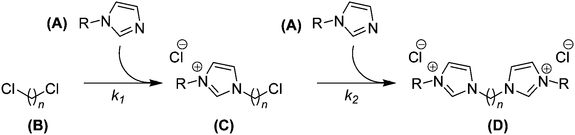
During studies into the ultra-high pressure synthesis of imidazolium salts, we encountered some rapid and high-yielding consecutive nucleophilic substitution reactions of N-alkyl imidazoles with dichloromethane and homologous α,ω-dichloroalkanes (Scheme 1).1 These are examples of parallel-consecutive (or competitive-consecutive) bimolecular reactions (Scheme 2), the kinetic equations of which, despite simplicity and similarity to those of other reaction mechanisms, are not so obviously solved. Resultantly, solving the inverse problem has posed a historical challenge.
 |
| | Scheme 1 Formation of bis(imidazoliumyl) alkane dichlorides, an example parallel-consecutive bimolecular reaction. | |
 |
| | Scheme 2 Kinetic scheme. | |
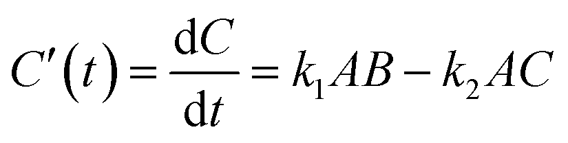
One of the early historical motivations to solve the problem was with application to the kinetics of diester hydrolysis – a two-step bimolecular sequence involving a common reagent – first reported by Ingold,2 and subsequently re-evaluated many times. There have been various approaches to the inverse problem of the parallel consecutive bimolecular reaction, and there are many examples of such reactions.3–14 Probably the most frequently reported data analysis methodology is that of Frost and Schwemer, and this dates back about 75 years.15 Use of the method, which requires the observation of particular pairs of reaction extents, is however more appropriate for continuously monitored reactions and less so for the post hoc measurements, such as those allowed by high-pressure batch-reactors, for example. This prompted the pursuit of alternative means of kinetic characterisation. In this note we demonstrate some mathematical features involving the intermediate species, C, that allow for an expedient solution to the inverse problem.
Theoretical treatment
The mechanism for the reaction illustrated in Scheme 2 is defined by the differential rate eqn (1)–(4),| |  | (1) |
| | 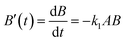 | (2) |
| |  | (3) |
| |  | (4) |
and in treatment of the kinetic data, the substitutions (5)–(8) are made for convenience,| | | Uni-functional species α = A/A0 | (5) |
| | | Bi-functional species β = B/B0 | (6) |
| | | Rate quotient κ = k2/k1 | (8) |
where A, B and C are concentrations, A0 and B0 are initial concentrations, α, β and γ are fractional concentrations, and k1 and k2 are rate constants for the two steps, respectively.
As has been discussed elsewhere, there are no closed form solutions to the differential rate eqn (1)–(4), which would be required to exactly express the integrated, time-dependent rate equations. Instead, solutions are obtained in terms of B rather than time, since in this basis the equations for all species do have closed form solutions.16 Correlations with time can then be subsequently achieved through graphical integration.17 Taken together, typical, exact algebraic solutions to the inverse kinetic problem appear precluded.
More widely known for his contribution to electrochemistry (of ‘Frost diagram’ fame),18 Frost and Schwemer were first to demonstrate the solution for the concentration A in terms of B (and not in terms of time).17 Alluding to the difficulty in solving the time-dependent integrals, their evaluation was not suggested, but instead the technique of time-ratios was promoted for the estimation of κ, which they attribute to Powell. Using variable transformations, McMillan later recast the differential rate equations into homogenous form and demonstrated that differential rate eqn (9), obtained by dividing (3) by (2), has the solution (10).19
| |  | (9) |
| |  | (10) |
Since
(10) does not involve the concentration
A, its analysis is independent of the initial mixing ratio,
ρ =
A0/
B0, provided only starting materials are initially present. For physically meaningful arguments
viz., 1 ≤
β ≤ 0, 1 ≤
γ ≤ 0 and
κ > 0,
(10) is not single-valued, but each pair of measured concentrations [
β,
γ] can belong to only one contour, which is described by a unique value of
κ. McMillan published
19 a plot of these parametric contours and suggested the use of these, or numerical methods, to approximate
κ from experimental data. There are, however, several additional relationships useful for describing the reaction profile and solving the inverse problem, which to our knowledge, are absent from the literature.
The stationary point
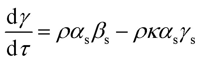
Following the derivation of Wen,16 using substitutions (5)–(8), eqn (3) can be recast in fractional concentrations as (11),| |  | (11) |
where the subscript s indicates a concentration at the stationary point, the initial mixing ratio ρ = A0/B0 and τ = B0k1t. Analogous to the situation encountered in analysis of steady state kinetics, at the quasi-stationary point in the reaction progression, (11) can be set to nought, and this leads to expression (12) for the rate constant quotient.| |  | (12) |
The particular concentrations [β, γ] that satisfy (12) are obtained using (10) to give (13) and (14), respectively. Although not considered here, in the limit of κ → 1, both concentrations are convergent to the constant, exp(−1) ≈ 0.368, and reflect a change in the particular solution16 to the differential equation set.| |  | (13) |
| |  | (14) |
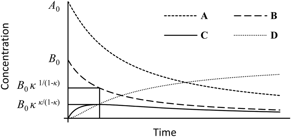
Conversion back to absolute concentrations is achieved by multiplying β and γ by B0, and are illustrated on the reaction profile, Fig. 1.
 |
| | Fig. 1 Example reaction profile for κ = 2.2 and A0/B0 = 2 with the stationary point concentrations indicated. | |
Solving the inverse problem
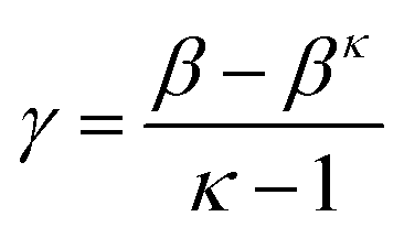
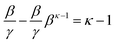
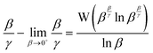
Isolating the concentration ratio β/γ in (10) gives (15), which is single-valued for all κ, and in the limit of β → 0+, converges to κ − 1 (16). This situation corresponds to an indefinite reaction time and extrapolating the quantity β/γ to its asymptotic minimum would be at best unreliable, or at worst, and more likely, guesswork. It does, however, yield a ceiling to the possible range, since β/γ ≥ κ − 1, always.
Although it is convenient, equality (12), β/γ = κ, is only true at the precise stationary point, i.e., when the value of β is exactly described by (13). There is deviation at all other reaction extents, which can be accounted for in a precise way using (17), but as an impredicative expression, evaluation cannot yield an unknown κ.
| |  | (15) |
| |  | (16) |
| |  | (17) |
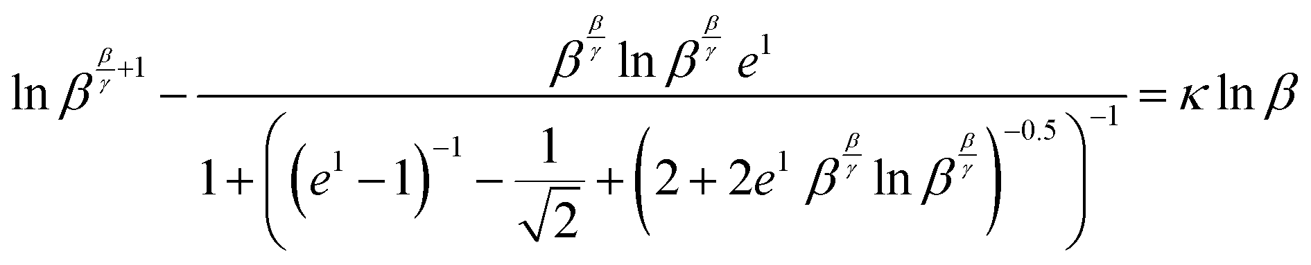
Instead,
eqn (18) obtained by isolating (
κ − 1) from
(15), unlike
(12), is true for all
β. It may appear that the multiple occurrences of (
κ − 1) prevent useful evaluation of
(18), but on account of the particular way the terms correspond, it is indeed soluble. Thus, continuing where McMillan left off with the plot of
(10),
eqn (18) is multiplied by ln
β and, exploiting a few logarithmic transformations, the equation becomes the log-linear parametric
eqn (19).
| |  | (18) |
| |  | (19) |
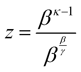
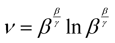
Through substitutions
(20) and (21),
eqn (19) can be cast in the form of Lambert's identity
(22),
20,21 the analytic inverse of which is the Lambert-W function
(23), and leads to
eqn (24).
| |  | (20) |
| |  | (21) |
| | ln![[thin space (1/6-em)]](https://www.rsc.org/images/entities/char_2009.gif) z + vz = 0 z + vz = 0 | (22) |
| |  | (24) |
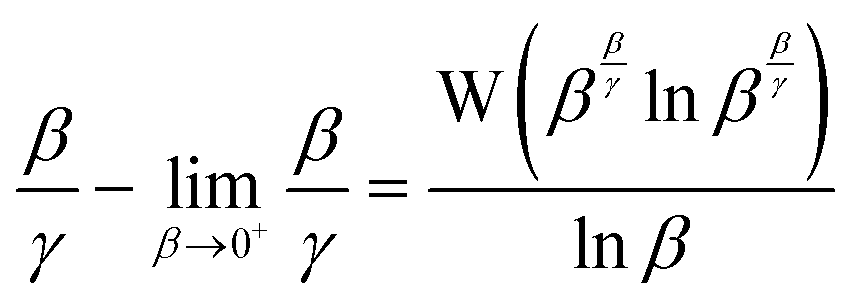
Hence, the deviation of the instantaneous value
β/
γ(15) from that in the limit of
β → 0
+(16) expressed in
(17) can be usefully evaluated without prior knowledge of
κ using
(25).
| |  | (25) |
Rearranging
(25) yields a time-independent expression for the rate quotient in terms of
β and
γ at any reaction extent
(26), and
eqn (27) is characteristic for the mechanism, where
κ > 1. Solving the inverse problem, a plot of
(27) is linear, and passes through the origin with a gradient equal the rate quotient,
κ.
| |  | (26) |
| |  | (27) |
Example and implementation
Whilst the Lambert-W function is not natively available in typical spreadsheet software packages, it can be implemented as a macro through evaluation of its series expansion (28), truncated to an arbitrary number of terms. A convenient algebraic alternative (29), due to Winitzki,22 provides an approximation of the appropriate branch (W0) in the necessary domain (−e−1 < x < 0). This approximation introduces a maximum error of less than 1 per cent.| |  | (28) |
| |  | (29) |
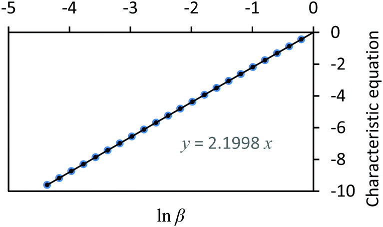
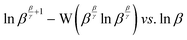
Using (29), a closed form expression can be cast (30) which approximates the rate quotient to a satisfactory accuracy provided the kinetic data are of sufficiently good quality. Applying (30) to the data presented in Fig. 1, a plot of the characteristic equation evaluated using the approximation is illustrated in Fig. 2.| |  | (30) |
In this example, the authentic rate constant quotient is κ = 2.2.
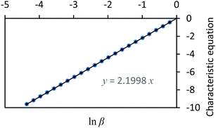 |
| | Fig. 2 A plot of the characteristic equation, lnββ/γ+1 − W(ββ/γlnββ/γ)versus lnβ. | |
As noted for (10), analysis using (26), (27) and (30) are similarly independent of concentration A, time, and also of the mixing ratio A0/B0 provided that only starting materials are present initially.
Conflicts of interest
There are no conflicts to declare.
Acknowledgements
The author wishes to thank Gavin Chiu for his helpful discussion and for proof reading, and also the referees and editors for their useful suggestions. This article is published in memory of Dr John Quigley, a good friend.
References
- L. M. Harwood, P. Pitt, J. L. Scott and D. Sousa, Tetrahedron, 2019, 75, 130639 CrossRef.
- C. Ingold, J. Chem. Soc., 1930, 1032 RSC.
- M. Zhu and B. Moasser, Tetrahedron Lett., 2012, 53, 2288 CrossRef CAS.
- C. D. Navo, N. Mazo, P. Oroz, M. I. Gutiérrez-Jiménez, J. Marín, J. Asenjo, A. Avenoza, J. H. Busto, F. Corzana, M. M. Zurbano and G. Jiménez-Osés, J. Org. Chem., 2020, 85, 3134 CrossRef CAS PubMed.
- L. I. Majoros, B. Dekeyser, R. Hoogenboom, M. W. Fijten, J. Geeraert, N. Haucourt and U. S. Schubert, J. Polym. Sci., Part A: Polym. Chem., 2010, 48, 570 CrossRef CAS.
- J. Casado, J. L. González and M. N. Moreno, React. Kinet. Catal. Lett., 1987, 33, 357 CrossRef CAS.
- C. Tsai, Y. Chen, J. Chen and L. Hwang, Polyhedron, 1992, 11, 1647 CrossRef CAS.
- R. Parette, R. McCrindle, K. S. McMahon and V. J. Watson,
et al.
, Environ. Forensics, 2017, 18, 307 CrossRef CAS.
- A. C. Conibear, K. A. Lobb and P. T. Kaye, Tetrahedron, 2010, 66, 8446 CrossRef CAS.
- C. Pavier and A. Gandini, Eur. Polym. J., 2000, 36, 1653 CrossRef CAS.
- L. Reich, Thermochim. Acta, 1997, 293, 179 CrossRef CAS.
- J. Burkus and C. Eckert, J. Am. Chem. Soc., 1958, 80, 5948 CrossRef CAS.
- C. Burkhard, Ind. Eng. Chem., 1960, 52, 678 CrossRef.
- P. Wells, J. Phys. Chem., 1959, 63, 1978 CrossRef CAS.
- W. C. Schwemer and A. A. Frost, J. Am. Chem. Soc., 1951, 73, 4541 CrossRef CAS.
- W. Y. Wen, J. Phys. Chem., 1972, 76, 704 CrossRef CAS.
- A. A. Frost and W. C. Schwemer, J. Am. Chem. Soc., 1952, 74, 1268 CrossRef CAS.
- A. A. Frost, J. Am. Chem. Soc., 1951, 73, 2680 CrossRef CAS.
- W. McMillan, J. Am. Chem. Soc., 1957, 79, 4838 CrossRef CAS.
- J. H. Lambert, Acta Helvetica, 1758, 3, 128 Search PubMed.
- D. Belkić, J. Math. Chem., 2019, 57, 59 CrossRef.
-
S. Winitzki, in Computational Science and Its Applications, ed. V. Kumar, M. L. Gavrilova, C. J. K. Tan and P. L’Ecuyer, Springer, Berlin, Heidelberg, 2003, pp. 780–789 Search PubMed.
|
| This journal is © the Owner Societies 2021 |
Click here to see how this site uses Cookies. View our privacy policy here. 
 Open Access Article
 This Open Access Article is licensed under a Creative Commons Attribution-Non Commercial 3.0 Unported Licence
 * and
Laurence M.
Harwood
* and
Laurence M.
Harwood