
 Open Access Article
 This Open Access Article is licensed under a Creative Commons Attribution-Non Commercial 3.0 Unported Licence
Interactions in protein solutions close to liquid–liquid phase separation: ethanol reduces attractions via changes of the dielectric solution properties
Jan
Hansen
 a,
Rajeevann
Uthayakumar
a,
Jan Skov
Pedersen
b,
Stefan U.
Egelhaaf
a and
Florian
Platten
*ac
a,
Rajeevann
Uthayakumar
a,
Jan Skov
Pedersen
b,
Stefan U.
Egelhaaf
a and
Florian
Platten
*ac
aCondensed Matter Physics Laboratory, Heinrich Heine University, Universitätsstraße 1, 40225 Düsseldorf, Germany. E-mail: florian.platten@hhu.de
biNANO Interdisciplinary Nanoscience Center and Department of Chemistry, Aarhus University, DK-8000 Aarhus C, Denmark
cInstitute of Biological Information Processing (IBI-4: Biomacromolecular Systems and Processes), Forschungszentrum Jülich, Wilhelm-Johnen-Straße, 52428 Jülich, Germany
First published on 29th September 2021
Abstract
Ethanol is a common protein crystallization agent, precipitant, and denaturant, but also alters the dielectric properties of solutions. While ethanol-induced unfolding is largely ascribed to its hydrophobic parts, its effect on protein phase separation and inter-protein interactions remains poorly understood. Here, the effects of ethanol and NaCl on the phase behavior and interactions of protein solutions are studied in terms of the metastable liquid–liquid phase separation (LLPS) and the second virial coefficient B2 using lysozyme solutions. Determination of the phase diagrams shows that the cloud-point temperatures are reduced and raised by the addition of ethanol and salt, respectively. The observed trends can be explained using the extended law of corresponding states as changes of B2. The results for B2 agree quantitatively with those of static light scattering and small-angle X-ray scattering experiments. Furthermore, B2 values calculated based on inter-protein interactions described by the Derjaguin-Landau-Verwey-Overbeek (DLVO) potential and considering the dielectric solution properties and electrostatic screening due to the ethanol and salt content quantitatively agree with the experimentally observed B2 values.
1 Introduction
When the attractions between protein molecules are strong enough, protein solutions can undergo liquid–liquid phase separation (LLPS) into two coexisting phases, one enriched and one depleted in proteins. Such protein phase separation has severe implications in fundamental and applied fields of research, including cell biology, medicine, pharmaceutical industry, food processing, and protein crystallography. For example, LLPS is exploited in vivo: subcellular compartments, so-called membraneless organelles, are formed via LLPS in the cytosol, representing a way of intracellular organization and regulation of biochemical reactions.1,2 Furthermore, genetic mutations or altered physicochemical conditions inside a cell are likely to affect inter-protein interactions and thus to disturb LLPS.3,4 However, LLPS can also modulate the pathways and kinetics of pathological protein aggregation leading to severe conditions for the patients.5,6 Protein solutions exhibit LLPS not only in vivo, but also in vitro.7,8 For example, antibodies, which are used as biopharmaceuticals in the treatment of various diseases,9 can undergo LLPS due to nonspecific antibody-antibody interactions.10–12 The dense-phase LLPS droplets might impair specific antibody-receptor interactions, enhance solution viscosity and cause immungenicity, posing a major challenge to the formulation development.13,14 LLPS can also be employed for identifying conditions under which high-quality crystals grow, which are needed for crystallographic structure determination.15 Yet, attempts to crystallize proteins are still frequently based on trial and error. Close to the LLPS binodal enhanced protein crystal nucleation rates have been observed by simulations and experiments,16,17 and therefore the location of the LLPS boundary has been regarded as a predictor for optimized crystallization conditions,18,19 as neither too weak nor too strong attractions are considered to be well suited for crystallization.20 Within the LLPS binodal, liquid-droplet nucleation or spinodal decomposition are typically faster than crystallization, thus leading to a two-step crystallization mechanism21,22 and altering crystallization kinetics.23,24Net attractions sufficient to induce LLPS can be achieved or avoided by dedicated changes of the physicochemical properties of the solution, e.g., by adding salts,25,26 excipients,27 or non-aqueous solvents.28,29 Moreover, organic solvents, such as alcohols, can act as precipitants30,31 and as crystallization agents.32,33 For example, in blood plasma fractionation,34,35 moderate ethanol concentrations (up to 40 vol%) are used to obtain therapeutic protein products. If added at high concentrations or used at elevated temperatures, ethanol can destabilize and unfold proteins,36,37 which might even lead to amyloid fibril formation.38–40 Its effects on individual protein molecules41,42 are largely ascribed to its hydrophobic properties.43 Ethanol is composed of a hydrophobic ethyl group and a hydrophilic hydroxyl group and can thus interact favorably with non-polar groups.31 However, far less (mechanistic) insight is established concerning the effects on inter-protein interactions, as relevant, e.g., for LLPS.
The second virial coefficient B2 represents an integral measure of the inter-protein interactions, which for a spherosymmetric potential U(r) with center-to-center distance r reads
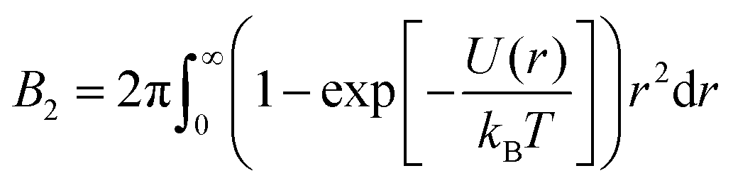 | (1) |
Concepts developed in soft-matter physics46–48 have proven helpful to rationalize the inter-protein interactions and the related phase behavior. Experimental protein phase diagrams, including LLPS phase coexistence curves (binodals), are strikingly similar to those of colloids with short-ranged attractions,49,50 as encountered, e.g., in square-well (SW) fluids49,51–53 or patchy particle systems.54–58 Furthermore, the structure factor of protein solutions close to phase separation has been described by Baxter's sticky particle model,19,59,60 for which an approximate analytical description is available.61,62 For colloids with short-ranged attractions, an extended law of corresponding states (ELCS) has been suggested by Noro and Frenkel,63 according to which short-ranged attractive systems can be mapped onto an equivalent SW system, and the applicability of the ELCS to the binodals of protein solutions has been demonstrated.53 The ELCS mapping thus reflects the insensitivity to the specific shape of the coarse-grained model potential, and in particular, it allows the estimation of B2 based on cloud-point measurements.64 In this context, the Derjaguin-Landau–Verwey–Overbeek (DLVO) theory has helped to rationalize the dependence of inter-protein interactions on simple salts, solvents or pH.65–69
In the present work, the effects of moderate ethanol concentrations on protein molecules, inter-protein interactions as well as LLPS coexistence curves are studied using lysozyme in brine as a model system. Small-angle X-ray scattering (SAXS) was used for determining the form factor of protein molecules, thus confirming that the alcohol and salt have no influence on the structure of the individual molecules on the relevant length scales. Cloud-point measurements are used to locate the LLPS binodal and to estimate B2 exploiting the ELCS. SAXS is also used to study the structure factor of concentrated protein solutions close to phase separation. From the analysis of the SAXS data, B2 is determined as a function of the ethanol content. The results confirm a universal temperature dependence of B2 with respect to the critical LLPS temperature, as suggested by the ELCS. The dependence of B2 on ethanol and salt content is quantitatively described by the DLVO theory taking only changes of the dielectric solution properties and the salt concentration into account. This work thus aims at a consistent picture of protein phase separation, a mechanistic explanation of solvent effects on inter-protein interactions and a resolution of controversial previous results.
2 Experimental methods
2.1 Sample preparation
Hen egg-white lysozyme was purchased from Sigma-Aldrich (prod. no. L6876) and used without further purification. For few SAXS experiments, lysozyme purchased from Roche Diagnostics (prod. no. 10837059001) was used, which led to consistent findings. Sodium chloride (NaCl), sodium acetate (NaAc) and ethanol (EtOH) were of reagent grade quality and used as received. Ultrapure water with a minimum resistivity of 18 MΩ cm was prepared using a water purification system.Water–ethanol mixtures containing 50 mM NaAc were used as buffer solutions and adjusted to pH reading 4.5 by adding small amounts of hydrochlorid acid. At pH 4.5 each lysozyme molecule carries approximately 11.4 positive net charges.70 Concentrated protein stock solutions were prepared by ultrafiltration, as described previously.29 The protein, ethanol and salt content of the stock solutions was checked by refractometry. With respect to pH value (4.5) and NaCl concentrations (0.7 M and 0.9 M), solution conditions are chosen to resemble those of our previous studies71,72 to allow for a quantitative comparison. Concerning the ethanol content, low and moderate concentrations (up to 30 vol% in increments of 10 vol%) are considered, similar to those of Liu et al.44 and Kundu et al.45 At pH 2.2, where lysozyme is expected to be less stable than at pH 4.5, ethanol-induced (partial) unfolding of lysozyme was only observed for ethanol concentrations larger than 30 vol%.73 Samples were prepared by mixing appropriate amounts of lysozyme, buffer and NaCl stock solutions. Protein concentrations cp are related to the protein volume fraction ϕ = cp/ρp, where ρp−1 = 0.740 cm3 g−1 is the specific volume of lysozyme.29 Mixing was performed at a temperature above the solution cloud-points to prevent immediate phase separation, typically at room temperature (21 ± 2) °C. Due to the high salt content, the samples were prone to crystallization26 and hence investigated immediately after preparation. Cloud points were typically studied using three independently prepared samples for each condition in order to allow for a statistical analysis. For SAXS, some of the samples were measured more than once in order to check the reproducibility of our results.
2.2 Cloud-point temperature measurements
Metastable LLPS coexistence curves were determined by cloud-point temperature measurements. Samples with a typical volume of 0.1 mL were filled into thoroughly cleaned glass capillary tubes, sealed, and placed into a thermostated water bath at a temperature well above the cloud-point. A wire thermometer was mounted in a separate, but closely placed glass tube filled with 0.1 mL water. Then, the temperature of the water bath was gradually lowered and the sample solution visually observed. The cloud point was identified by the sample becoming turbid. Further details have been given previously.292.3 Estimation of the second virial coefficient based on cloud-point measurements
The extended law of corresponding states (ELCS), suggested by Noro and Frenkel,63 applies to colloidal system dominated by short-range attractions. It has been demonstrated53 that it also applies to protein solutions, despite their complex interactions. According to the ELCS, these systems obey the same equation of state and hence their LLPS phase boundaries collapse onto one another, if expressed in suitable reduced quantities. The ELCS can be exploited to estimate the second virial coefficient.53,64 This is based on the critical temperature of the binodal and an effective hard-core diameter, which takes into account the repulsive inter-particle interactions and can be inferred from a one-parameter fit to the experimental gas branch of the binodal. Once these parameters are determined, the universal temperature dependence (with respect to the critical temperature) of the reduced second virial coefficient can be exploited to estimate the second virial coefficient at a given temperature. Details on this procedure have been given previously.532.4 Small-angle X-ray scattering: instrumentation
Small-angle X-ray scattering (SAXS) was employed to determine the form factor of individual protein molecules to reveal possible shape or size changes as well as the structure factor characterizing the effective inter-protein interactions at temperatures close to, but above the solution cloud-points. SAXS experiments were performed using the laboratory-based facilities at the Interdisciplinary Nanoscience Center (iNANO) at Aarhus University, Denmark,74 as well as at Center for Structural Studies at Heinrich Heine University Düsseldorf, Germany. In Aarhus, a NanoSTAR SAXS camera (Bruker AXS) optimized for solution scattering75 with a home-built scatterless pinhole in front of the sample76 was used to measure the scattered intensity of sample and buffer solutions. The solutions were filled in a thin flow-through glass capillary and thermostated using a Peltier element (Anton Paar). In Düsseldorf, SAXS measurements on sample and buffer solutions were performed on a XENOCS 2.0 device with a Pilatus 3 300 K detector. The solutions were injected into a thin flow-through capillary cell mounted on a thermal stage. Experiments were performed at 20.0 °C and 25.0 °C, respectively. Typical acquistion times of 10 and 5 min were used for dilute and concentrated solutions (typically, 6 and 70 mg mL−1), respectively. The data were background subtracted and converted to absolute scale using water in Aarhus75 and glassy carbon in Düsseldorf as standards. The final intensity is displayed as a function of the magnitude of the scattering vector,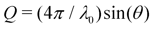 , where the X-ray wavelength, λ0, is 1.54 Å and 2θ is the angle between the incident and scattered X-rays and calibration was performed using silver behenate.
2.5 Small-angle X-ray scattering: data analysis
Protein molecules tend to have anisotropic shapes; according to X-ray crystallography, lysozyme is approximately a prolate ellipsoid with an extension of 30 × 30 × 45 Å3.77 For a monodisperse solution of particles with only a small anisotropy, the interactions can be assumed to be independent of the orientation. Then, the absolute scattered intensity I(Q) can be described by the decoupling approximation:78–80| I(Q) = KcpM P(Q)Seff(Q). | (2) |
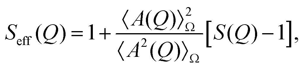 | (3) |
![[thin space (1/6-em)]](https://www.rsc.org/images/entities/char_2009.gif) 320 g mol−1, and the contrast factor K ∼ (Δρ)2 related to the electron density difference Δρ between particle and solvent, which can be computed.81,82
320 g mol−1, and the contrast factor K ∼ (Δρ)2 related to the electron density difference Δρ between particle and solvent, which can be computed.81,82
For very dilute systems, S(Q) ≈ 1 and the Q dependence of I(Q) is determined by the size, shape and structure of the individual particles via P(Q). In particular, the radius of gyration Rg, a measure of the particle size, can be inferred from the low-Q scattering. To describe the shape and structure of the lysozyme molecules, two different models for P(Q) are considered here. On a coarse level,80 the form factor of lysozyme can be modelled as a prolate ellipsoid of revolution with minor and major axes as parameters. Since the atomic coordinates of lysozyme are known (PDB file 1LYZ83), the form factor can be calculated accurately using the programme CRYSOL,84 which calculates the excess scattering and adds a 3 Å hydration shell with the shell electron density ρsh as a parameter.
In concentrated solutions, the structure factor S(Q) contains information on the spatial arrangement of the particles and thus reflects inter-particle interactions. In a one-component system, the coexistence of two stable or metastable fluid phases is only possible if the particle interactions are net attractive. The square-well (SW) potential arguably represents the simplest model to describe the effective interactions of such a system.49 It consists of a hard-core repulsion of range σ (the diameter of the particle), which leads to excluded volume effects, and a constant attractive part, which has depth ε and extends to a distance λσ from the center. The adhesive hard-sphere (AHS) potential proposed by Baxter represents a specific limit of the SW potential:85 the SW depth ε becomes infinite while the SW width (λ − 1)σ becomes infinitesimal (i.e., λ → 1), such that the contribution to B2 remains finite and nonzero:
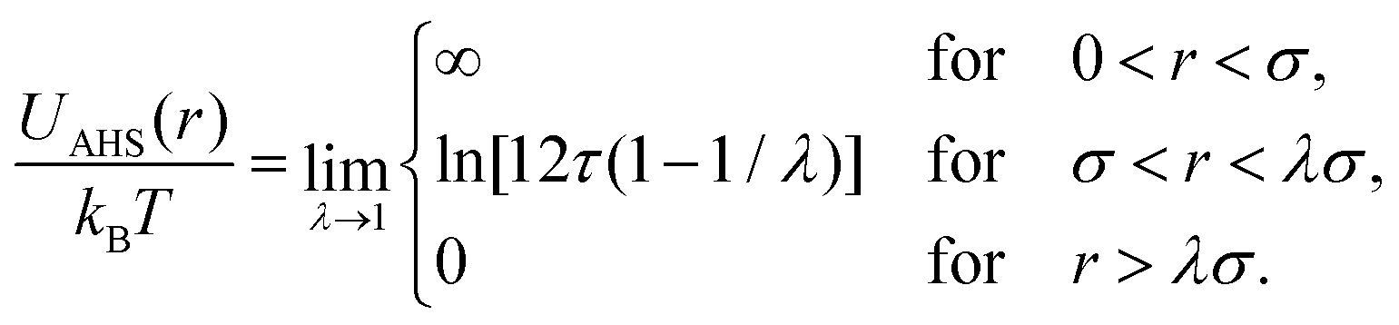 | (4) |
 | (5) |
 | (6) |
The scattered intensity based on eqn (2) with a constant scattering background is fitted to the measured scattered intensity using a least-square routine. Since background subtraction is particularly delicate at very low Q, model fits are compared with experimental data for Q ≥ 0.015 Å−1. The contrast factor of lysozyme in the different water–ethanol mixtures is calculated using the MULCh software.81 To account for the experimental uncertainty in cp, a deviation of up to 10% from its nominal value is allowed in fitting.
3 Results and discussion
First, the effect of moderate ethanol concentration on the size and shape of individual protein molecules is investigated by SAXS. In a second step, LLPS coexistence curves are determined for various ethanol and salt compositions. Then, the structure factor of moderately concentrated systems close to LLPS is examined by SAXS measurements of concentrated samples. Both from the cloud-point measurements (by exploiting the ELCS) and from the SAXS data (by applying Baxter's AHS model), the normalized second virial coefficient b2 is inferred. Finally, the dependence of b2 on ethanol and salt content is rationalized based on DLVO theory.3.1 Lysozyme molecular structure in water–ethanol mixtures
The scope of the present work is on the LLPS of folded, globular proteins,93 whose interactions are tuned by the addition of ethanol and NaCl. However, ethanol can also denature and aggregate proteins.37,94,95 Therefore, the shape and size of individual lysozyme molecules in water–ethanol mixtures are determined.Fig. 1 shows the scattered intensity I(Q) of dilute protein solutions (cp ≈ 6 mg mL−1) under two particular conditions: (i) proteins in an aqueous solution with 0.9 M NaCl, which is used to screen electrostatic repulsions (squares), and (ii) proteins in a water–ethanol mixture with the highest ethanol concentration used in this work (30 vol% EtOH) with 0.9 M NaCl (diamonds). Experiments on intermediate ethanol concentrations show similar behavior. In Fig. 1(A), the experimental data for both conditions are shown with I(Q) normalized by the ethanol-dependent contrast factor K, the molecular weight M and the protein concentration cp. Since S(Q) ≈ 1 in this case, eqn (2) implies that the data reflect the form factor P(Q). The data obtained for the two different conditions do not show any significant difference in the covered Q range, indicating that the shape and size of the lysozyme molecules are not affected by 30 vol% ethanol. The Q dependence of the data exhibits a plateau with I(Q)/KcpM ≈ P(Q) ≈ 1 at low Q and a minimum at high Q which suggests a globular object. A Guinier analysis indicates radii of gyration Rg = 15.5 Å (0 vol% EtOH) and Rg = 14.9 Å (30 vol% EtOH). Radii of gyration determined in repeat measurements and experiments at intermediate ethanol concentrations range from approximately 15 to 17 Å, indicating an experimental uncertainty of 1.1 Å.
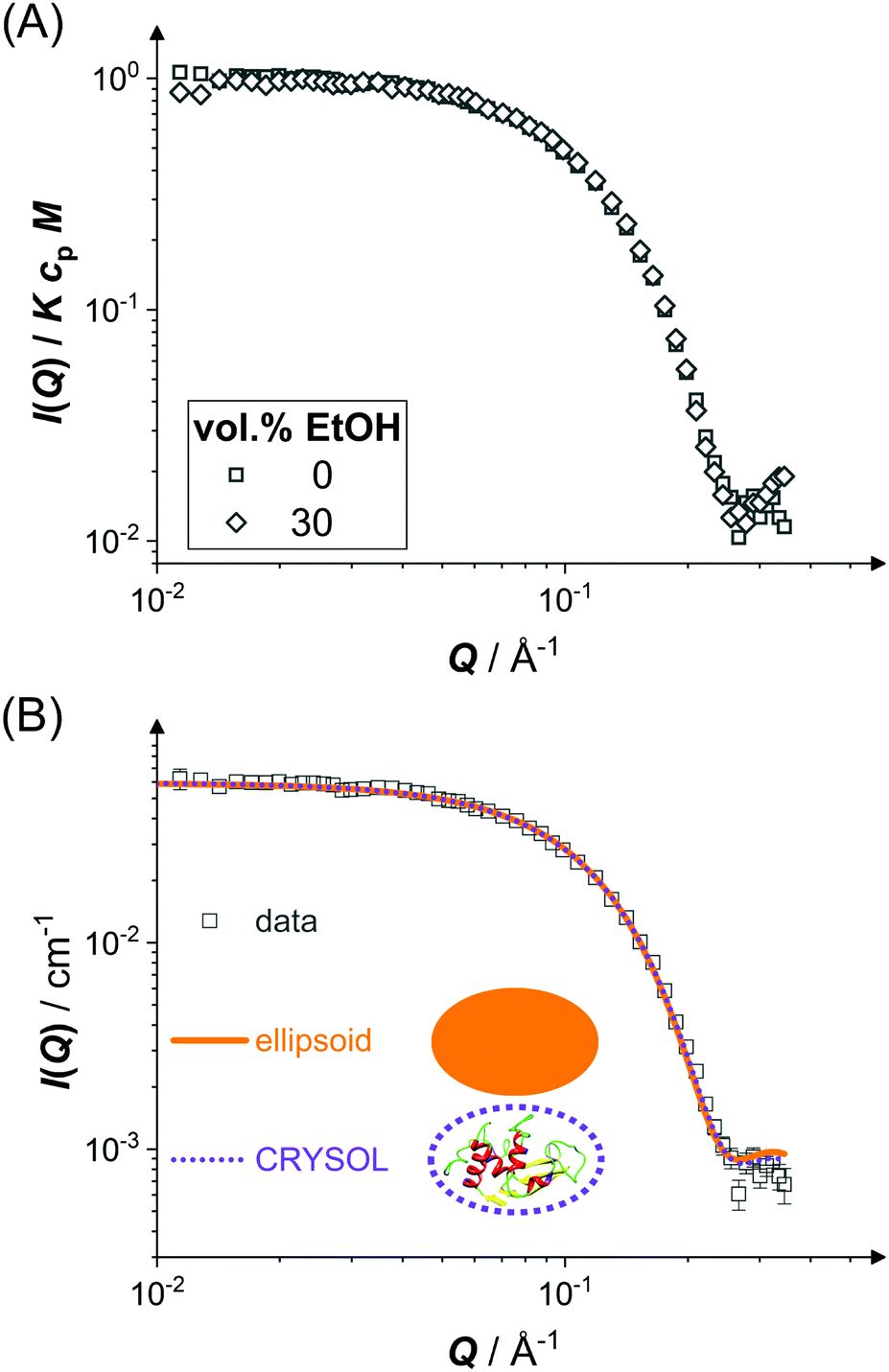 | ||
| Fig. 1 Form factor of lysozyme molecules (cp ≈ 6 mg mL−1) in brine (0.9 M NaCl) without and with 30 vol% EtOH (squares and diamonds, respectively): (A) scattered intensity I(Q) normalized by the contrast factor K, the molecular weight M, and the protein concentration cp as a function of the magnitude of the scattering vector Q. (B) Scattered intensity I(Q) as experimentally determined (squares as in (A)) and model fits (lines as indicated). Schematic drawings (not to scale) illustrate the two models. For the crystal structure, only the backbone is shown. | ||
In Fig. 1(B), fits based on two different form factor models (lines) to the experimental data of the aqueous solution (symbols) are shown. The first form factor model is based on a prolate ellipsoid of revolution with a semi-minor axis 16.0 Å and an axial ratio fixed at 1.5 (solid line), which describes the experimental data reasonably well. The second one is calculated via the CRYSOL programme84 (dotted line) with ρsh in agreement with previous work.84 It quantitatively reproduces the experimental data and thus agrees with the ellipsoid model except for minor differences at very high Q.
The experimental data and the analysis demonstrate that lysozyme molecules retain their compact native shape under all conditions studied. This is in line with a previous finding73 that higher ethanol concentrations are required to induce unfolding, which might change protein size and shape.
3.2 Liquid–liquid phase separation of lysozyme solutions in water–ethanol mixtures
Samples might show a macroscopic phase transition accompanied by a clouding of the system which indicates LLPS. The temperature at which the system becomes cloudy depends on the strength of the net attractions. Higher cloud-point temperatures indicate stronger net attractions. Cloud-point temperature measurements thus represent a simple way to characterize the inter-particle interactions.64Fig. 2(A) and (B) show the low-volume fraction branch of LLPS phase coexistence curves of lysozyme solutions in brine (0.9 and 0.7 M NaCl represented by open and closed large symbols, respectively) with and without ethanol being added. In the absence of ethanol, the data agree with literature results (small symbols).28 With increasing protein concentration cp, the cloud-point temperature TLLPS first increases steeply, reflecting an enhanced effect of inter-protein attractions. Then, TLLPS saturates at high protein concentrations, indicating the proximity to the critical point.53 In the latter case, critical scalings can be used for describing the T − cp dependence:8,25,71,96
 | (7) |
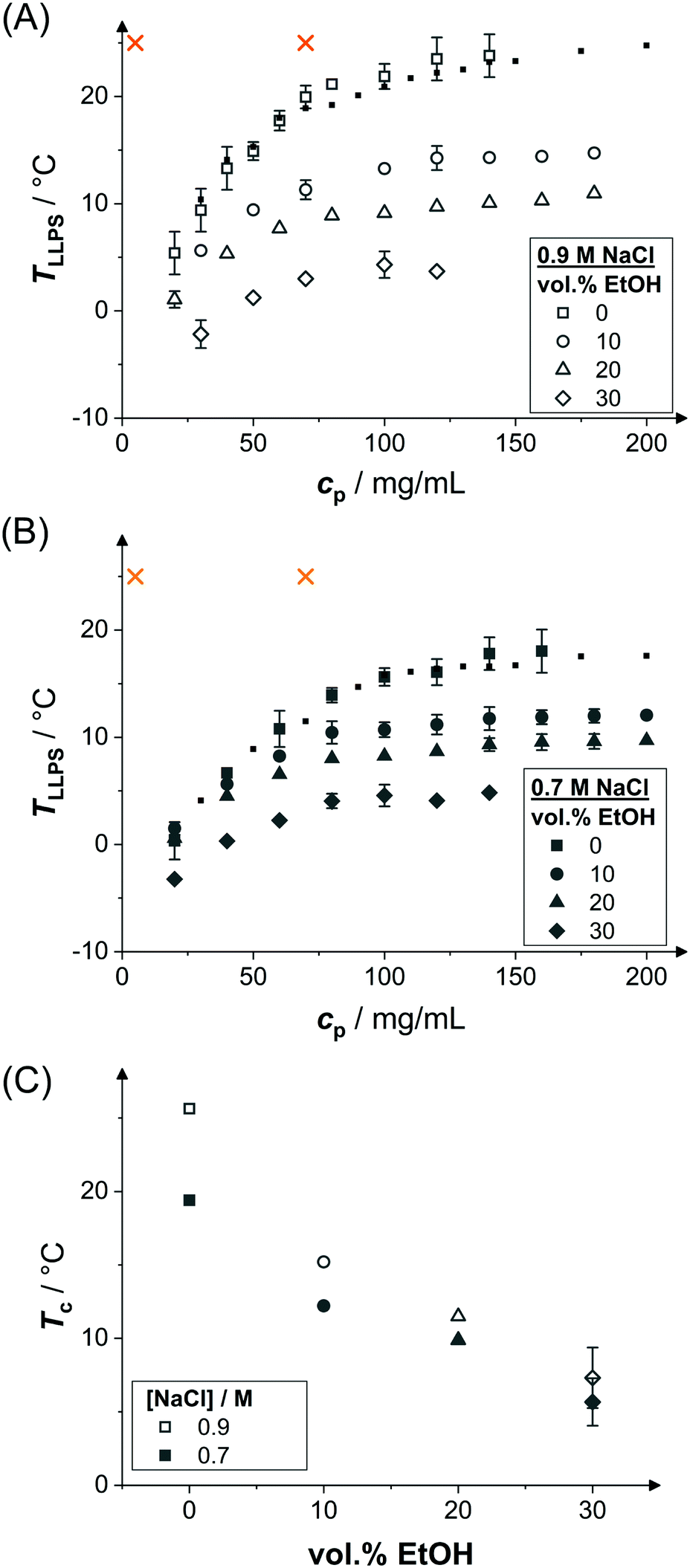 | ||
| Fig. 2 Effect of ethanol on the LLPS. Cloud-point temperature TLLPS as a function of protein concentration cp representing the LLPS coexistence curves in the presence of (A) 0.9 M NaCl and (B) 0.7 M NaCl as well as various ethanol concentrations as indicated (large symbols). Literature data28 in the absence of ethanol (small symbols). Typical solution conditions probed in SAXS experiments (crosses); at this temperature, b2 is also estimated based on the cloud-points. (C) Estimated critical temperature Tc as a function of the ethanol content for the two NaCl concentrations as indicated. | ||
The attractions can be quantified by interaction parameters, such as the second virial coefficient b2. Based on cloud-point measurements, b2 at a given temperature close to the binodal can be estimated by a comparison of the experimental binodal with those of short-ranged SW fluids,53 as suggested by the extended law of corresponding states.63 Following this approach, b2 has been determined at the temperature indicated by crosses in Fig. 2(A and B) for the different solution compositions probed. The results will be discussed in Section 3.4.
3.3 The interactions in protein solutions close to phase separation
Pair interactions in protein solutions can be inferred from the concentration-dependence of the scattered intensity97 or from the Q dependence of the scattering intensity through structure factor models.98 However, close to the LLPS spinodal, critical or off-critical scattering contributions99 are expected to occur and analytical mean-field models usually employed to analyze scattering data are expected to fail. Thus, to be able to determine the pair interaction parameters through structure factor modelling, we focus on moderately concentrated solutions at temperatures that are at least a few degrees above the expected LLPS spinodal temperatures.100Fig. 3(A) shows the normalized scattered intensity I(Q)/KcpM of concentrated protein solutions (cp ≈ 70 mg mL−1 in the presence of ethanol and 50 mg mL−1 in the absence of ethanol) under conditions close to phase separation but far enough away from the LLPS spinodal, as indicated in Fig. 2(A and B). The experiments were performed at a fixed temperature. However, due to the different ethanol and NaCl concentrations (as indicated by the symbol type and filling, respectively) and hence different T/Tc, the distance to the LLPS boundary increases as Tc decreases with ethanol content (Fig. 2(C)) and decreases as Tc increases with NaCl concentration. In order to compare the different solution compositions with each other, all data are shown in a single graph.
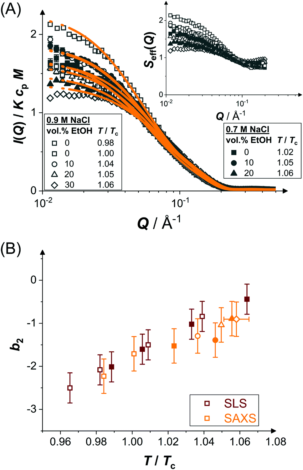 | ||
| Fig. 3 (A) Scattering vector-dependent normalized scattered intensity, I(Q)/KcpM, of concentrated protein solutions (cp ≈ 70 mg mL−1) close to phase separation (temperature T relative to the respective critical temperature Tc, ethanol and salt content as indicated): experimental data (symbols) and model fits (lines). Inset: Effective structure factor Seff(Q) as inferred from the data, according to eqn (2). Only data with Q ≤ 0.2 Å are shown, as they are very noisy beyond this value. (B) Normalized second virial coefficient b2 as a function of temperature T normalized by the critical temperature Tc. Data based on SAXS (orange symbols) and static light scattering28 (SLS, red symbols). Open and closed symbols correspond to 0.9 and 0.7 M NaCl, respectively. Ethanol content is reflected in the symbol shape as in (A). | ||
According to eqn (2), the Q dependence of the scattering curves reflects both the form and structure factor. Since P(Q) was found to be unaltered by the different solution conditions, the variations in I(Q) are largely due to changes of S(Q). At intermediate and high Q, the curves do not reveal marked differences. However, at low Q, the scattered intensity tends to increase as T/Tc decreases and hence the distance to the LLPS boundary also decreases. The effective structure factors Seff(Q) are shown as an inset. The low-Q increase with Seff(Q → 0) > 1 is due to enhanced inter-protein attractions upon approaching the LLPS (as well as minor changes of cp). A qualitatively similar behavior has been observed for other protein systems.59,60,99
The model of eqn (2) is fitted to the experimental data where the form factor is described by a prolate ellipsoid of revolution80 with fixed parameters (cf. Section 3.1) and the analytical structure factor of adhesive hard-spheres in the Percus-Yevick approximation62,86 is implemented. As suggested by the ELCS, the specific shape of the interaction potential is not crucial. The experimental data are quantitatively reproduced by the model fits, in particular the low Q upturn upon approaching phase separation. For each scattering curve, the fit provides a refined value of the stickiness parameter τ, which can be converted to a normalized second virial coefficient b2viaeqn (6). This determination of b2 is based on an extended Q range and hence more reliable than a determination using S(Q → 0) only. The resulting b2 values are displayed in Fig. 3(B) as a function of the reduced temperature T/Tc of the solution. The statistical uncertainty of b2 is estimated to be ±0.4 based on the analysis of several independently prepared samples at the same condition. In the temperature range investigated, b2 increases monotonously with reduced temperature. The interaction parameter retrieved from fitting, τ, (and thus also b2) as well as the quality of the fit are very similar if the form factor is modelled using the atomic coordinates implemented in a home-written programme that also takes the hydration layer into account.101
In addition to the b2 data retrieved by the SAXS analysis, static light scattering (SLS) data28 on the aqueous system are shown. Both data sets quantitatively agree with each other. Thus, despite the proximity to LLPS, SAXS yields reliable results for the interaction parameters. Due to the quantitative agreement with the SLS data, the SAXS data thus provide further support for a universal temperature dependence (with respect to Tc) of b2 of protein solutions, as previously noted for lysozyme53 and γB-crystallin.99
3.4 Ethanol effect on the second virial coefficient of lysozyme solutions: experiments and DLVO model
Upon addition of ethanol, the LLPS coexistence curve of lysozyme shifts to lower temperatures, as discussed in Section 3.2. Accordingly, for increasing ethanol content, T/Tc increases for a fixed temperature T, such as the temperature of the SAXS experiments (mainly 25 °C but also a few at 20 °C). The correspondingly reduced net attractions are reflected in the reduced low Q scattering. Hence, b2 is expected to increase with ethanol content. To quantify this dependence, values of b2 were determined by comparing the low-concentration branches of the binodals (Fig. 2(A and B)) with those of SW fluids and exploiting the ELCS.53 The results reveal a weak, but systematic increase of b2 with ethanol content (Fig. 4(A and B)). Moreover, the values quantitatively agree with b2 values determined by SAXS model fits (Fig. 3 and 4(A,B)).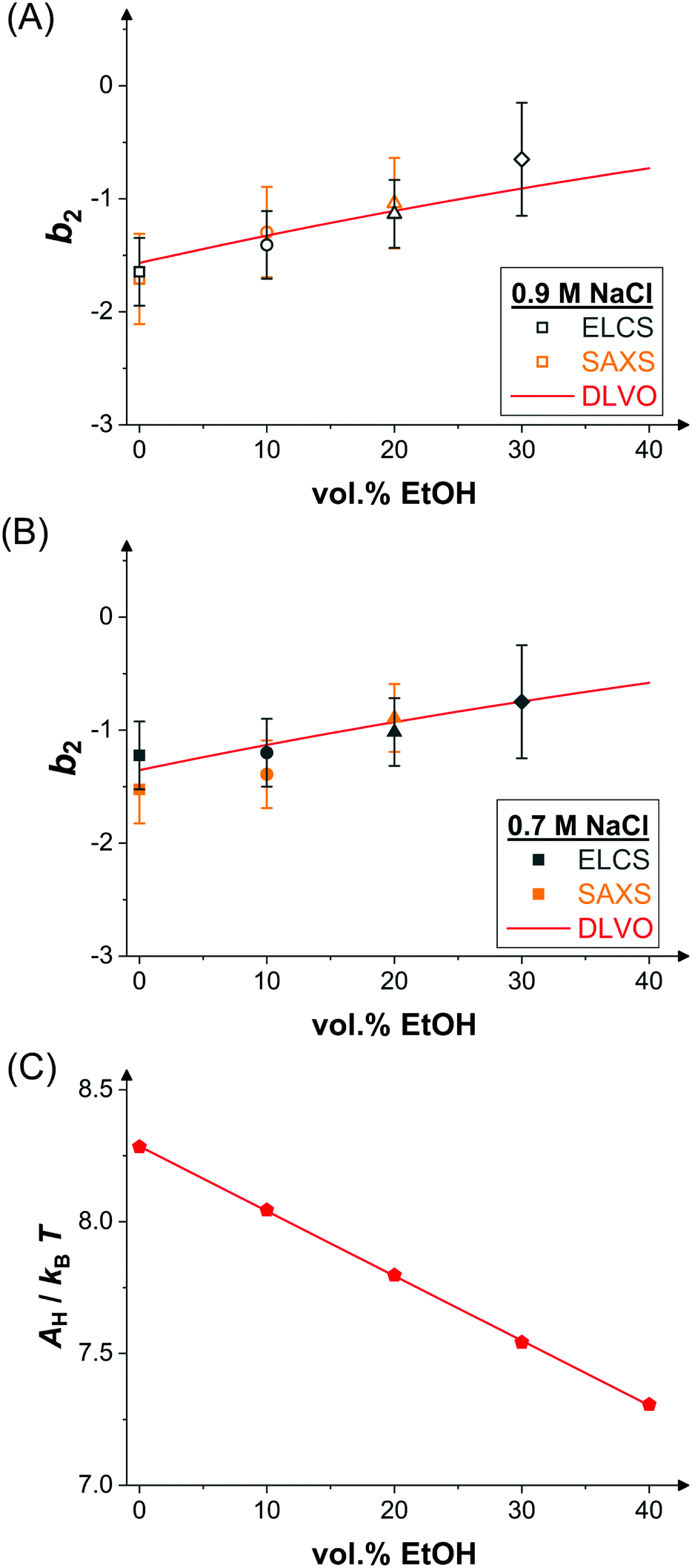 | ||
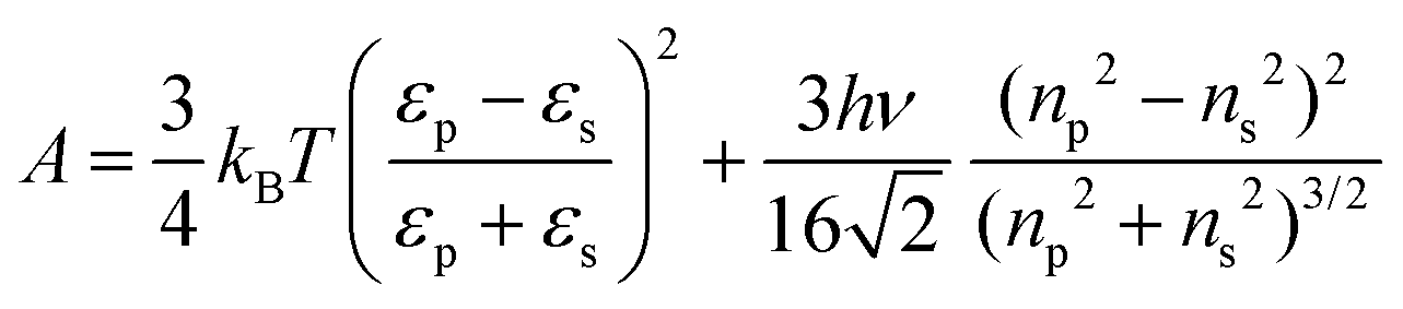
| Fig. 4 Effect of ethanol on inter-protein interactions. (A) Normalized second virial coefficient b2 as function of ethanol content at 25 °C and in the presence of 0.9 M NaCl. Data inferred from the cloud-point measurements (Fig. 2(A)) via the ELCS (grey symbols) and from the analysis of the SAXS data (Fig. 3(A)) (orange symbols) as well as calculated values based on the DLVO theory (line). (B) Data and theoretical predictions as in (A), but in the presence of 0.7 M NaCl. (C) Hamaker constant calculated based on eqn (12) (symbols) and linear fit (line). | ||
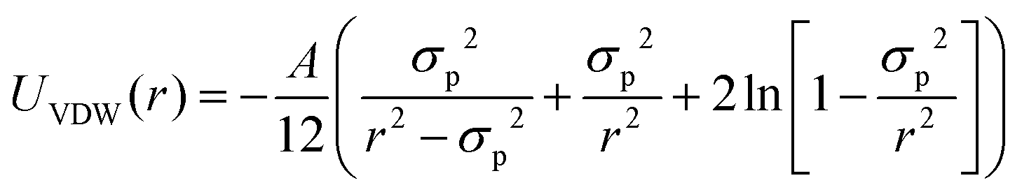
In order to rationalize the dependence of b2 on ethanol and salt content, protein interactions are modelled by the DLVO potential:102
| UDLVO(r) = UHS(r) + USC(r) + UVDW(r) | (8) |
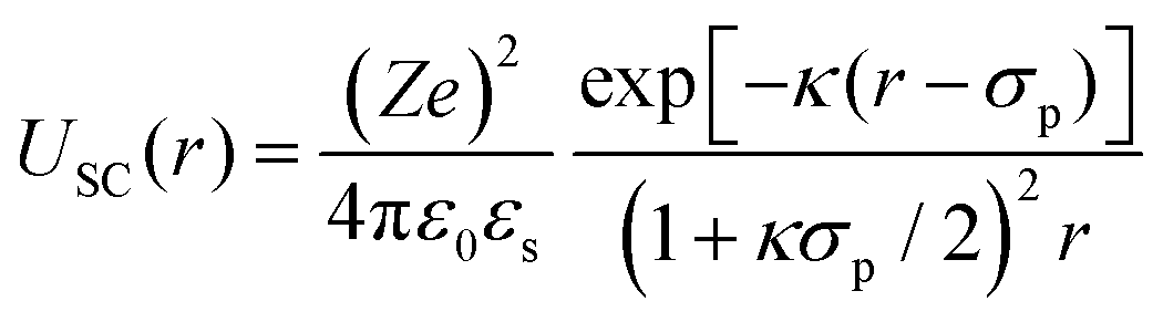 | (9) |
 | (10) |
 | (11) |
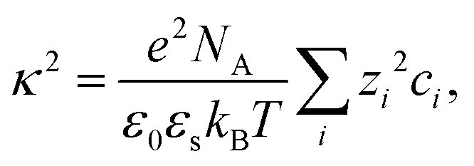
 | (12) |
The normalized second virial coefficient, b2, can be computed based on the DLVO potential viaeqn (1). To avoid divergence of the integral, a cut-off length δ related to the Stern layer is used as lower integration limit. Its value, δ ≈ 0.16 nm, has previously been adjusted to match SLS data.64 Note that σp + δ ≈ σ; i.e., the diameter of the adhesive hard sphere σ assumed in the structure factor modelling agrees with that of the hard sphere amended with a cut-off layer used in the DLVO model. This DLVO description might thus implicitly also account for non-DLVO effects, such as hydration, the hydrophobic effect and hydrogen bonding.110 The results of the DLVO model are shown in Fig. 4(A and B) as solid lines. The model b2 monotonously increases with ethanol content and quantitatively agrees with the experimental data (symbols). Thus, the ethanol-dependent changes of the inter-protein interactions are fully accounted for by its effect on the dielectric solution properties and thus on the Hamaker constant and the screening length. Salt effects are contained in κ (eqn (10)).
Liu et al.44 studied lysozyme pair interactions in water–ethanol mixtures at neutral pH. At three different NaCl concentrations, an increase of b2 at low and a plateau at moderate ethanol concentrations was observed by light scattering. To describe their data, they used a modified DLVO model. The Hamaker constant A was assumed to be constant irrespective of the ethanol content and the net charge Z was treated as an adjustable parameter in contrast to our approach (Fig. 4(C)). In addition, the DLVO potential was supplemented by an alcohol-dependent patchy SW potential and the interaction strength of the patch was allowed to vary with alcohol concentration. Compared with this more complex model, our DLVO calculation is simpler and does not require any free parameter. However, if applied to their solution conditions, our model (with Z = 8.4) predicts a monotonous weak increase of b2 with ethanol content, similar to our experimental finding, and thus does not fully explain their observation. It is conceivable that the slightly different trends observed are due to differences in accounting for the peculiar physicochemical properties of water–ethanol mixtures, such as the interpretation of pH values.111
Cosolvents can be preferentially bound to or excluded from the protein surface.112 The composition of the surface layer can affect the inter-protein interactions113 and, as a consequence, the protein phase behaviour.71 Up to moderate ethanol concentrations, some preferential binding of ethanol to lysozyme has been reported,114 although significant excess binding was not observed in another study.115 This is consistent with our SAXS data (Fig. 1), which do not show a dependence on the ethanol content, and our DLVO model, which quantitatively agrees with the data without considering preferential binding. Moreover, the ELCS suggests that, as long as a system is governed by short-range attractions, the collective behaviour can be described by integral parameters, such as b2, whereas the details of the interaction potential are less relevant. Nevertheless, it cannot be excluded that preferential binding as well as patchiness and directionality,116,117 asymmetric shapes,118 charge patterns119 or other phenomena play some role. Their effects, however, are expected to be small or balance each other since our DLVO model is sufficient to quantitatively describe the data. Furthermore, also the effects of adding salt, glycerol or dimethyl sulfoxide can be rationalized by a DLVO model.28,64,66,67 This supports the view that at least the crucial effects are captured in a coarse-grained DLVO approach based on macroscopic solution properties despite the inherent complexity and molecular effects of inter-protein interactions.
4 Conclusion
The phase behavior and the interactions of proteins in water–ethanol mixtures were studied. The addition of moderate amounts of ethanol was found to decrease LLPS temperatures indicating reduced net attractions and, consistently, the low-Q SAXS intensity of concentrated protein solutions decreases and the b2 values increase. The data suggest universal net interactions close to phase separation, supporting the extended law of corresponding states. The increase of b2 with ethanol can be quantitatively captured by a DLVO model taking into account the effect of ethanol on the dielectric solution properties. Thus, the DLVO theory can provide a mechanistic description of protein interactions also in complex solution environments.Conflicts of interest
There are no conflicts to declare.Acknowledgements
We thank Jan K. G. Dhont (FZ Jülich, Germany) and Ramón Castañeda-Priego (Leon, Mexico) for stimulating and very helpful discussions, and Beatrice Plazzotta for assistance with the SAXS measurements in Aarhus. F. P. acknowledges financial support by the Strategic Research Fund of the Heinrich Heine University (F 2016/1054-5) and the German Research Foundation (PL 869/2-1). We thank the Center for Structural Studies (CSS) for access to the SAXS instrument. CSS is funded by the Deutsche Forschungsgemeinschaft (DFG Grant numbers 417919780 and INST 208/761-1 FUGG).Notes and references
- A. A. Hyman, C. A. Weber and F. Jülicher, Annu. Rev. Cell Dev. Biol., 2014, 30, 39–58 CrossRef CAS PubMed.
- C. P. Brangwynne, P. Tompa and R. V. Pappu, Nat. Phys., 2015, 11, 899–904 Search PubMed.
- Y. Shin and C. P. Brangwynne, Science, 2017, 357, eaaf4382 CrossRef PubMed.
- S. Alberti and A. A. Hyman, Nat. Rev. Mol. Cell Biol., 2021, 22, 196–213 CrossRef CAS PubMed.
- W. M. Babinchak and W. K. Surewicz, J. Mol. Biol., 2020, 432, 1910–1925 CrossRef CAS PubMed.
- S. Ray, N. Singh, R. Kumar, K. Patel, S. Pandey, D. Datta, J. Mahato, R. Panigrahi, A. Navalkar, S. Mehra, L. Gadhe, D. Chatterjee, A. S. Sawner, S. Maiti, S. Bhatia, J. A. Gerez, A. Chowdhury, A. Kumar, R. Padinhateeri, R. Riek, G. Krishnamoorthy and S. K. Maji, Nat. Chem., 2020, 12, 705–716 CrossRef CAS PubMed.
- C. Ishimoto and T. Tanaka, Phys. Rev. Lett., 1977, 39, 474–477 CrossRef CAS.
- M. Muschol and F. Rosenberger, J. Chem. Phys., 1997, 107, 1953–1962 CrossRef CAS.
- A. L. Nelson, E. Dhimolea and J. M. Reichert, Nat. Rev. Drug Discovery, 2010, 9, 767–774 CrossRef CAS PubMed.
- Y. Wang, A. Lomakin, R. F. Latypov, J. P. Laubach, T. Hideshima, P. G. Richardson, N. C. Munshi, K. C. Anderson and G. B. Benedek, J. Chem. Phys., 2013, 139, 121904 CrossRef PubMed.
- Y. Wang, R. F. Latypov, A. Lomakin, J. A. Meyer, B. A. Kerwin, S. Vunnum and G. B. Benedek, Mol. Pharmaceutics, 2014, 11, 1391–1402 CrossRef CAS PubMed.
- S. Da Vela, F. Roosen-Runge, M. W. A. Skoda, R. M. J. Jacobs, T. Seydel, H. Frielinghaus, M. Sztucki, R. Schweins, F. Zhang and F. Schreiber, J. Phys. Chem. B, 2017, 121, 5759–5769 CrossRef CAS PubMed.
- B. A. Salinas, H. A. Sathish, S. M. Bishop, N. Harn, J. F. Carpenter and T. W. Randolph, J. Pharm. Sci., 2010, 99, 82–93 CrossRef CAS PubMed.
- A. S. Raut and D. S. Kalonia, Mol. Pharmaceutics, 2016, 13, 1431–1444 CrossRef CAS PubMed.
- N. E. Chayen and E. Saridakis, Nat. Methods, 2008, 5, 147–153 CrossRef CAS PubMed.
- P. R. ten Wolde and D. Frenkel, Science, 1997, 277, 1975–1978 CrossRef CAS PubMed.
- O. Galkin and P. G. Vekilov, Proc. Natl. Acad. Sci. U. S. A., 2000, 97, 6277–6281 CrossRef CAS PubMed.
- G. A. Vliegenthart and H. N. W. Lekkerkerker, J. Chem. Phys., 2000, 112, 5364–5369 CrossRef CAS.
- F. Zhang, R. Roth, M. Wolf, F. Roosen-Runge, M. W. A. Skoda, R. M. J. Jacobs, M. Stzucki and F. Schreiber, Soft Matter, 2012, 8, 1313–1316 RSC.
- A. George and W. W. Wilson, Acta Crystallogr., Sect. D: Struct. Biol., 1994, 50, 361–365 CrossRef CAS PubMed.
- P. G. Vekilov, Nanoscale, 2010, 2, 2346–2357 RSC.
- F. Zhang, F. Roosen-Runge, A. Sauter, R. Roth, M. W. A. Skoda, R. M. J. Jacobs, M. Sztucki and F. Schreiber, Faraday Discuss., 2012, 159, 313–325 RSC.
- Y. Liu, X. Wang and C. B. Ching, Cryst. Growth Des., 2010, 10, 548–558 CrossRef CAS.
- A. Sauter, F. Roosen-Runge, F. Zhang, G. Lotze, R. M. J. Jacobs and F. Schreiber, J. Am. Chem. Soc., 2015, 137, 1485–1491 CrossRef CAS PubMed.
- M. L. Broide, T. M. Tominc and M. D. Saxowsky, Phys. Rev. E: Stat., Nonlinear, Soft Matter Phys., 1996, 53, 6325–6335 CrossRef CAS PubMed.
- H. Sedgwick, K. Kroy, A. Salonen, M. B. Robertson, S. U. Egelhaaf and W. C. K. Poon, Eur. Phys. J. E: Soft Matter Biol. Phys., 2005, 16, 77–80 CrossRef CAS PubMed.
- A. S. Raut and D. S. Kalonia, Mol. Pharmaceutics, 2016, 13, 774–783 CrossRef CAS PubMed.
- C. Gögelein, D. Wagner, F. Cardinaux, G. Nägele and S. U. Egelhaaf, J. Chem. Phys., 2012, 136, 015102 CrossRef PubMed.
- F. Platten, J. Hansen, J. Milius, D. Wagner and S. U. Egelhaaf, J. Phys. Chem. B, 2015, 119, 14986–14993 CrossRef CAS PubMed.
- S. N. Timasheff and T. Arakawa, J. Cryst. Growth, 1988, 90, 39–46 CrossRef CAS.
- H. Yoshikawa, A. Hirano, T. Arakawa and K. Shiraki, Int. J. Biol. Macromol., 2012, 50, 865–871 CrossRef CAS PubMed.
- E. J. Cohn, W. L. Hughes and J. H. Weare, J. Am. Chem. Soc., 1947, 69, 1753–1761 CrossRef CAS PubMed.
- A. McPherson, Methods, 2004, 34, 254–265 CrossRef CAS PubMed.
- E. J. Cohn, L. E. Strong, W. L. Hughes, D. J. Mulford, J. N. Ashworth, M. Melin and H. L. Taylor, J. Am. Chem. Soc., 1946, 68, 459–475 CrossRef CAS PubMed.
- A. A. Green and W. L. Hughes, Methods Enzymol., 1955, 1, 67–90 CAS.
- J. F. Brandts and L. Hunt, J. Am. Chem. Soc., 1967, 89, 4826–4838 CrossRef CAS PubMed.
- R. M. Parodi, E. Bianchi and A. Ciferri, J. Biol. Chem., 1973, 248, 4047–4051 CrossRef CAS.
- S. Goda, K. Takano, K. Yutani, Y. Yamagata, R. Nagata, H. Akutsu, S. Maki and K. Namba, Protein Sci., 2000, 9, 369–375 CrossRef CAS PubMed.
- M. Holley, C. Eginton, D. Schaefer and L. R. Brown, Biochem. Biophys. Res. Commun., 2008, 373, 164–168 CrossRef CAS PubMed.
- A. Giugliarelli, L. Tarpani, L. Latterini, A. Morresi, M. Paolantoni and P. Sassi, J. Phys. Chem. B, 2015, 119, 13009–13017 CrossRef CAS PubMed.
- K. Ikeda and K. Hamaguchi, J. Biochem., 1970, 68, 785–794 CrossRef CAS PubMed.
- P. D. Thomas and K. A. Dill, Protein Sci., 1993, 2, 2050–2065 CrossRef CAS PubMed.
- Y. Nozaki and C. Tanford, J. Biol. Chem., 1971, 246, 2211–2217 CrossRef CAS.
- W. Liu, D. Bratko, J. M. Prausnitz and H. W. Blanch, Biophys. Chem., 2004, 107, 289–298 CrossRef CAS PubMed.
- S. Kundu, V. Aswal and J. Kohlbrecher, Chem. Phys. Lett., 2017, 670, 71–76 CrossRef CAS.
- J. D. Gunton, A. Shiryayev and D. L. Pagan, Protein condensation. Kinetic pathways to crystallization and disease, Cambridge University Press, 2007 Search PubMed.
- J. J. McManus, P. Charbonneau, E. Zaccarelli and N. Asherie, Curr. Opin. Colloid Interface Sci., 2016, 22, 73–79 CrossRef CAS.
- A. Stradner and P. Schurtenberger, Soft Matter, 2020, 16, 307–323 RSC.
- N. Asherie, A. Lomakin and G. B. Benedek, Phys. Rev. Lett., 1996, 77, 4832–4835 CrossRef CAS PubMed.
- W. C. K. Poon, Phys. Rev. E: Stat., Nonlinear, Soft Matter Phys., 1997, 55, 3762–3764 CrossRef CAS.
- A. Lomakin, N. Asherie and G. B. Benedek, J. Chem. Phys., 1996, 104, 1646–1656 CrossRef CAS.
- Y. Duda, J. Chem. Phys., 2009, 130, 116101 CrossRef PubMed.
- F. Platten, N. E. Valadez-Pérez, R. Castañeda Priego and S. U. Egelhaaf, J. Chem. Phys., 2015, 142, 174905 CrossRef PubMed.
- R. P. Sear, J. Chem. Phys., 1999, 111, 4800–4806 CrossRef CAS.
- A. Lomakin, N. Asherie and G. B. Benedek, Proc. Natl. Acad. Sci. U. S. A., 1999, 96, 9465–9468 CrossRef CAS PubMed.
- H. Liu, S. K. Kumar and F. Sciortino, J. Chem. Phys., 2007, 127, 084902 CrossRef PubMed.
- C. Gögelein, G. Nägele, R. Tuinier, T. Gibaud, A. Stradner and P. Schurtenberger, J. Chem. Phys., 2008, 129, 085102 CrossRef PubMed.
- M. Kastelic, Y. V. Kalyuzhnyi, B. Hribar-Lee, K. A. Dill and V. Vlachy, Proc. Natl. Acad. Sci. U. S. A., 2015, 112, 6766–6770 CrossRef CAS PubMed.
- J. Möller, S. Grobelny, J. Schulze, S. Bieder, A. Steffen, M. Erlkamp, M. Paulus, M. Tolan and R. Winter, Phys. Rev. Lett., 2014, 112, 028101 CrossRef PubMed.
- M. Wolf, F. Roosen-Runge, F. Zhang, R. Roth, M. W. Skoda, R. M. Jacobs, M. Sztucki and F. Schreiber, J. Mol. Liq., 2014, 200, 20–27 CrossRef CAS.
- C. Regnaut and J. C. Ravey, J. Chem. Phys., 1989, 91, 1211–1221 CrossRef CAS.
- S. V. G. Menon, C. Manohar and K. S. Rao, J. Chem. Phys., 1991, 95, 9186–9190 CrossRef CAS.
- M. G. Noro and D. Frenkel, J. Chem. Phys., 2000, 113, 2941–2944 CrossRef CAS.
- F. Platten, J. Hansen, J. Milius, D. Wagner and S. U. Egelhaaf, J. Phys. Chem. Lett., 2016, 7, 4008–4014 CrossRef CAS PubMed.
- M. Muschol and F. Rosenberger, J. Chem. Phys., 1995, 103, 10424–10432 CrossRef CAS.
- W. C. K. Poon, S. U. Egelhaaf, P. A. Beales, A. Salonen and L. Sawyer, J. Phys.: Condens. Matter, 2000, 12, L569 CrossRef CAS.
- H. Sedgwick, J. E. Cameron, W. C. K. Poon and S. U. Egelhaaf, J. Chem. Phys., 2007, 127, 125102 CrossRef CAS PubMed.
- G. Pellicane, J. Phys. Chem. B, 2012, 116, 2114–2120 CrossRef CAS PubMed.
- S. Kumar, I. Yadav, D. Ray, S. Abbas, D. Saha, V. K. Aswal and J. Kohlbrecher, Biomacromolecules, 2019, 20, 2123–2134 CrossRef CAS PubMed.
- C. Tanford and R. Roxby, Biochem., 1972, 11, 2192–2198 CrossRef CAS PubMed.
- J. Hansen, F. Platten, D. Wagner and S. U. Egelhaaf, Phys. Chem. Chem. Phys., 2016, 18, 10270–10280 RSC.
- L. Hentschel, J. Hansen, S. U. Egelhaaf and F. Platten, Phys. Chem. Chem. Phys., 2021, 23, 2686–2696 RSC.
- K. Sasahara and K. Nitta, Proteins, 2006, 63, 127–135 CrossRef CAS PubMed.
- M. A. Behrens, J. Bergenholtz and J. S. Pedersen, Langmuir, 2014, 30, 6021–6029 CrossRef CAS PubMed.
- J. S. Pedersen, J. Appl. Crystallogr., 2004, 37, 369–380 CrossRef CAS.
- J. Lyngsø and J. S. Pedersen, J. Appl. Crystallogr., 2021, 54, 295–305 CrossRef.
- C. C. F. Blake, D. F. Koenig, G. A. Mair, A. C. T. North, D. C. Phillips and V. R. Sarma, Nature, 1965, 206, 757–761 CrossRef CAS PubMed.
- M. Kotlarchyk and S.-H. Chen, J. Chem. Phys., 1983, 79, 2461–2469 CrossRef CAS.
- S. H. Chen, Annu. Rev. Phys. Chem., 1986, 37, 351–399 CrossRef CAS.
- J. S. Pedersen, Adv. Colloid Interface Sci., 1997, 70, 171–210 CrossRef CAS.
- A. E. Whitten, S. Cai and J. Trewhella, J. Appl. Crystallogr., 2008, 41, 222–226 CrossRef CAS.
- K. L. Sarachan, J. E. Curtis and S. Krueger, J. Appl. Crystallogr., 2013, 46, 1889–1893 CrossRef CAS.
- R. Diamond, J. Mol. Biol., 1974, 82, 371–391 CrossRef CAS PubMed.
- D. Svergun, C. Barberato and M. H. J. Koch, J. Appl. Crystallogr., 1995, 28, 768–773 CrossRef CAS.
- R. J. Baxter, J. Chem. Phys., 1968, 49, 2770–2774 CrossRef CAS.
- S. V. G. Menon, V. K. Kelkar and C. Manohar, Phys. Rev. A: At., Mol., Opt. Phys., 1991, 43, 1130–1133 CrossRef CAS PubMed.
- M. Bergström, J. S. Pedersen, P. Schurtenberger and S. U. Egelhaaf, J. Phys. Chem. B, 1999, 103, 9888–9897 CrossRef.
- A. P. R. Eberle, R. Castañeda-Priego, J. M. Kim and N. J. Wagner, Langmuir, 2012, 28, 1866–1878 CrossRef CAS PubMed.
- A. Tardieu, A. Le Verge, M. Malfois, F. Bonneté, S. Finet, M. Riès-Kautt and L. Belloni, J. Cryst. Growth, 1999, 196, 193–203 CrossRef CAS.
- Y. Liu, W.-R. Chen and S.-H. Chen, J. Chem. Phys., 2005, 122, 044507 CrossRef PubMed.
- S.-H. Chen, M. Broccio, Y. Liu, E. Fratini and P. Baglioni, J. Appl. Crystallogr., 2007, 40, s321–s326 CrossRef CAS.
- S. Kundu, V. Aswal and J. Kohlbrecher, Chem. Phys. Lett., 2016, 657, 90–94 CrossRef CAS.
- P. G. Vekilov, Soft Matter, 2010, 6, 5254–5272 RSC.
- S. Tanaka, Y. Oda, M. Ataka, K. Onuma, S. Fujiwara and Y. Yonezawa, Biopolymers, 2001, 59, 370–379 CrossRef CAS PubMed.
- L. R. Nemzer, B. N. Flanders, J. D. Schmit, A. Chakrabarti and C. M. Sorensen, Soft Matter, 2013, 9, 2187–2196 RSC.
- H. E. Stanley, Introduction to Phase Transitions and Critical Phenomena (International Series of Monographs on Physics), Clarendon Press, 1971 Search PubMed.
- F. Bonneté, S. Finet and A. Tardieu, J. Cryst. Growth, 1999, 196, 403–414 CrossRef.
- F. Zhang, M. W. A. Skoda, R. M. J. Jacobs, R. A. Martin, C. M. Martin and F. Schreiber, J. Phys. Chem. B, 2007, 111, 251–259 CrossRef CAS PubMed.
- S. Bucciarelli, N. Mahmoudi, L. Casal-Dujat, M. Jehannin, C. Jud and A. Stradner, J. Phys. Chem. Lett., 2016, 7, 1610–1615 CrossRef CAS PubMed.
- M. Manno, C. Xiao, D. Bulone, V. Martorana and P. L. San Biagio, Phys. Rev. E: Stat., Nonlinear, Soft Matter Phys., 2003, 68, 011904 CrossRef PubMed.
- E. M. Steiner, J. Lyngsø, J. E. Guy, G. Bourenkov, Y. Lindqvist, T. R. Schneider, J. S. Pedersen, G. Schneider and R. Schnell, Proteins, 2018, 86, 912–923 CrossRef CAS PubMed.
- J. N. Israelachvili, Intermolecular and surface forces, Academic Press, London; San Diego, 2nd edn, 1991 Search PubMed.
- G. Åkerlöf, J. Am. Chem. Soc., 1932, 54, 4125–4139 CrossRef.
- T. A. Scott, J. Phys. Chem., 1946, 50, 406–412 CrossRef CAS PubMed.
- S. M. Puranik, A. C. Kumbharkhane and S. C. Mehrotra, J. Mol. Liq., 1994, 59, 173–177 CrossRef CAS.
- J. Herráez and R. Belda, J. Sol. Chem., 2006, 35, 1315–1328 CrossRef.
- F. I. El-Dossoki, J. Chin. Chem. Soc., 2007, 54, 1129–1137 CrossRef CAS.
- M. Farnum and C. Zukoski, Biophys. J., 1999, 76, 2716–2726 CrossRef CAS PubMed.
- J. J. Dwyer, A. G. Gittis, D. A. Karp, E. E. Lattman, D. S. Spencer, W. E. Stites and B. García-Moreno E., Biophys. J., 2000, 79, 1610–1620 CrossRef CAS PubMed.
- G. Pellicane, D. Costa and C. Caccamo, J. Phys. Chem. B, 2004, 108, 7538–7541 CrossRef CAS.
- R. G. Bates, M. Paabo and R. A. Robinson, J. Phys. Chem., 1963, 67, 1833–1838 CrossRef CAS.
- E. S. Courtenay, M. W. Capp, C. F. Anderson and M. T. Record, Biochemistry, 2000, 39, 4455–4471 CrossRef CAS PubMed.
- I. L. Shulgin and E. Ruckenstein, J. Phys. Chem. B, 2008, 112, 14665–14671 CrossRef CAS PubMed.
- M. G. Ortore, P. Mariani, F. Carsughi, S. Cinelli, G. Onori, J. Teixeira and F. Spinozzi, J. Chem. Phys., 2011, 135, 245103 CrossRef PubMed.
- Y. Shindo and K. Kimura, J. Chem. Soc., Faraday Trans. 1, 1984, 80, 2199–2207 RSC.
- C. J. Roberts and M. A. Blanco, J. Phys. Chem. B, 2014, 118, 12599–12611 CrossRef CAS PubMed.
- F. Roosen-Runge, F. Zhang, F. Schreiber and R. Roth, Sci. Rep., 2014, 4, 7016 CrossRef CAS PubMed.
- A. Grünberger, P.-K. Lai, M. A. Blanco and C. J. Roberts, J. Phys. Chem. B, 2013, 117, 763–770 CrossRef PubMed.
- E. Allahyarov, H. Löwen, A. A. Louis and J. P. Hansen, Europhys. Lett., 2002, 57, 731–737 CrossRef CAS.
| This journal is © the Owner Societies 2021 |