Structure and dynamics of highly concentrated LiTFSI/acetonitrile electrolytes

Abstract

High salt concentration has been shown to induce increased electrochemical stability in organic solvent-based electrolytes. Accompanying the change in bulk properties is a structural ordering on mesoscopic length scales and changes in the ion transport mechanism have also been suggested. Here we investigate the local structure and dynamics in highly concentrated acetonitrile electrolytes as a function of salt concentration. Already at low concentrations ordering on microscopic length scales in the electrolytes is revealed by small angle X-ray scattering, as a result of correlations of Li⁺ coordinating clusters. For higher salt concentrations a charge alternation-like ordering is found as anions start to take part in the solvation. Results from quasi-elastic neutron spectroscopy reveal a jump diffusion dynamical process with jump lengths virtually independent of both temperature and Li-salt concentration. The jump can be envisaged as dissociation of a solvent molecule or anion from a particular Li⁺ solvation structure. The residence time, 50–800 ps, between the jumps is found to be highly temperature and Li-salt concentration dependent, with shorter residence times for higher temperature and lower concentrations. The increased residence time at high Li-salt concentration can be attributed to changes in the interaction of the solvation shell as a larger fraction of TFSI anions take part in the solvation, forming more stable solvation shells.

---

1. Introduction

Since their initial commercialisation in 1991 lithium-ion batteries (LIBs) have become standard in portable electronics and are currently expanding into the electric vehicle market. Even though the basic chemistry concept is the same (intercalation of Li-ions in a graphite-based anode and a transition metal-oxide cathode) the performance of LIBs has improved considerably. The improvement stems mainly from significant advances in the electrode materials,^1,2 whereas much less development has been made on the electrolyte side. For further development of LIBs, in terms of both capacity and safety, the electrolyte is a key component. While electrolytes with larger voltage windows would allow the implementation of high voltage cathodes, an increased thermal stability of the electrolyte would enhance the safety compared to the current concepts based on highly flammable organic solvents.³

Several electrolyte concepts have been proposed in order to improve both the capacity and the safety aspects.^4,5 An interesting approach is based on the finding that highly concentrated solutions (e.g. 3 to >20 m depending on the solvent/salt combination) of certain Li-salts in polar solvents behave completely different compared to standard electrolyte solutions where the Li-salt concentration is lower (∼1 m).^6–13 One example is acetonitrile (AN), which is one of the most oxidation-tolerant organic solvents that could enable the use of high voltage electrodes (>5 V). However, AN has not found extensive poor reductive stability.⁹ Yamada et al. found that highly concentrated solutions (i.e., over 3 m) of acetonitrile and the Li-salt LiTFSI (TFSI, bis(trifluoromethylsufonyl)imide) have a remarkable electrochemical stability window. Additionally, these electrolytes allow for fast charging and long-lasting LIBs.^9,14 Moreover, Nie et al. reported that highly concentrated mixtures of propylene carbonate (PC) and LiPF₆ allow for successful intercalation of Li⁺ into graphite and the formation of a stable passivation layer that results in a good cycle performance.⁷ Furthermore, Watanabe et al. have found that at the equimolar concentrations of tetraglyme (TEGDME) and LiTFSI the electrochemical stability window is increased.^8,13 However, the origin of the improved performance of highly concentrated electrolyte solutions is still not clear.

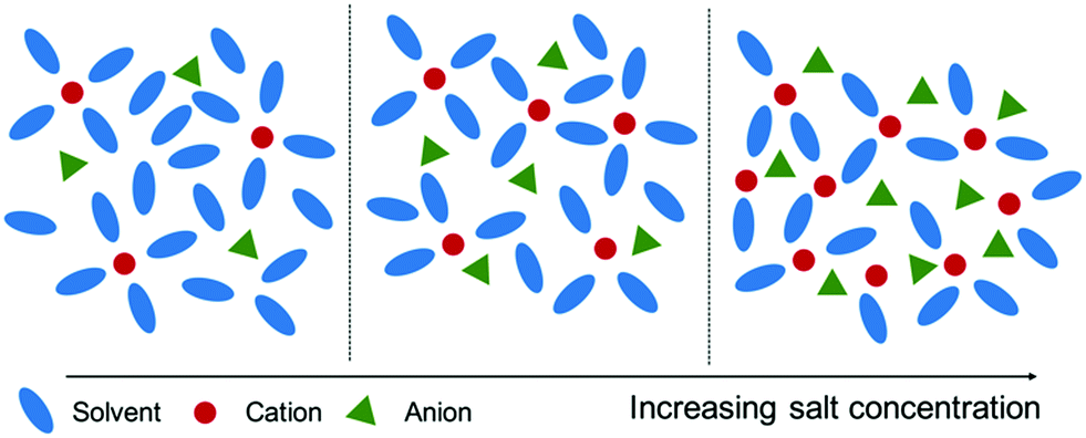
The structure of highly concentrated solutions can be expected to be quite different from what is found in ordinary liquids and in dilute electrolytes. By increasing the salt concentration, more and more solvent molecules will be tied up in the solvation shell around the Li-ions until a point when there are no free solvent molecules left, see schematic in Fig. 1. In the case of the equimolar solutions of TEGDME and LiTFSI, it has been shown that one solvent molecule forms a rather stable complex with a Li-ion.^8,15,16 Since this complex effectively forms a large cation, charge balanced by the anion from the Li-salt, these highly concentrated solutions have been named solvated ionic liquids and indeed they share many of the advantageous properties of ionic liquids (ILs).¹² In addition, it has been shown that solvated ionic liquids share the typical nanostructure, resulting from charge alternation, typically found in ILs, manifested as a peak, at low momentum transfers (Q), in small angle X-ray scattering (SAXS) data not present in ordinary simple liquids.¹⁷ This phenomenon has also been observed in siloxane-based highly concentrated electrolytes where the charge alternation peak in SAXS data increases in intensity as the salt concentration in the electrolyte is increased.¹⁸

Fig. 1 Schematic of the local electrolyte structure as a function of concentration.

The presence of an ordering beyond nearest neighbours can be expected to also influence the transport mechanism in highly concentrated electrolytes. Ion transport in standard (dilute) electrolytes is governed by a vehicular-type mechanism where the Li-ion is moving together with its solvation shell.¹⁹ The nanostructure and charge ordering present in highly concentrated electrolytes makes it plausible that the ion transport mechanism is more complex, but at present there is a limited understanding of the local dynamics and its relation to the nanostructure. One proposed mechanism is ligand exchange, where ion transport takes place through association/dissociation of solvent molecules, or anions at very high salt concentrations, in the solvation shell of the Li-ion.²⁰ It has also been suggested that in some systems the ion transport takes place in 3D percolating networks as a result of microscopic heterogeneities in the solution induced by the high salt concentration.²¹ From NMR-experiments a mixed vehicular and jump diffusion mechanism has also been proposed by Dokko et al.²²

So far, most results in literature on local dynamics of highly concentrated electrolytes are derived from computer simulations,^{20,21,23–26} while experimental studies are still few. Quasi-elastic neutron scattering (QENS) is a particularly suitable experimental tool as it covers the typical length scales of structural ordering in highly concentrated electrolytes. For ionic liquids QENS has revealed a complex picture of the dynamics with several different processes contributing to the local dynamics.^27–32 However, to the best of our knowledge no studies have been reported on the local dynamics in highly concentrated electrolytes using QENS.

In order to enable the design of improved electrolytes it is key to understand the microscopic structure and dynamics that gives rise to the macroscopic favourable properties of highly concentrated electrolytes. In particular, the nature of solvation shells and their dynamics is of importance not only for fast ion transport, but also for e.g., electrochemical processes and the formation of the solid electrolyte interphase.^33–35 In this work we focus on the local structure and dynamics in an archetypal highly concentrated electrolyte and their connection to the macroscopic transport properties, i.e., the conductivity. We investigate electrolytes based on acetonitrile and the Li-salt LiTFSI, Scheme 1, as a function of salt concentration, from the rather dilute regime to very high concentrations. This system was chosen as the flexible nature of TFSI allows for liquid electrolytes to be stable, i.e., crystallization can be avoided, even at very high salt concentrations for large temperature ranges. With SAXS we find the development of a nanostructure in solutions already from rather low salt concentrations originating from a particular organisation of AN molecules around the Li-ions. With QENS we probe the local dynamics directly on these length scales and show that the local dynamics can be described by a jump-diffusion type motion in the highly concentrated electrolytes as the first step of the conduction process.

Scheme 1 Chemical structure of acetonitrile and LiTFSI.

2. Experimental

2.1 Materials

Lithium bis(trifluoromethanesulfonyl)imide (LiTFSI) from Solvionic (99.9% < 20 ppm H₂O) was dissolved in acetonitrile (AN) (Sigma Aldrich, 99.8%) for the SAXS experiments and in deuterated acetonitrile (d-AN) (Sigma Aldrich, 99.96%) for the QENS experiments. Seven samples were prepared for SAXS measurements with AN to LiTFSI ratios 20 : 1, 10 : 1, 5 : 1, 4 : 1, 3 : 1, 2 : 1, 3 : 2 (number of solvent molecules per Li⁺) and three samples with AN to LiTFSI ratios 20 : 1, 5 : 1 and 2 : 1 for the QENS experiments. The samples were kept and handled in inert atmosphere.

2.2 Conductivity

Conductivity measurements were performed on a Novocontrol Broadband Dielectric Spectrometer in the frequency range 10⁻²–10⁷ Hz. The sample was placed between two brass electrodes, separated by a 1 mm Teflon spacer. Measurements were taken in the temperature range 225–350 K. The DC-conductivity was determined from the plateau value of the frequency dependent conductivity.

2.3 Small angle X-ray scattering

SAXS experiments were performed at the I911-4 beamline at MAXlab. With an incident wavelength of 0.91 Å and a sample to detector distance of 31.3 cm the momentum transfer range Q = 0.2–3.5 Å⁻¹ was covered in one setting. Measurements were performed at ambient conditions. Data was normalized to the incoming beam intensity and the corresponding empty cell contribution was subtracted. Calibration to absolute units was not performed. Samples were loaded in 2 mm glass capillaries sealed with epoxy resin in a glove box.

2.4 Quasi-elastic neutron scattering

QENS experiments were performed on the backscattering spectrometer IN16B ILL, Grenoble, France.³⁶ IN16B accesses an energy range of ±30 μeV with a resolution of 0.75 μeV for momentum transfer values 0.6–1.9 Å⁻¹.³⁷ Data was reduced and analysed using LAMP³⁸ and DAVE³⁹ software packages. Samples were loaded into annular cylindrical aluminium cans with a sample thickness of 0.15–0.25 mm, sealed with indium wire and QENS spectra were recorded in the temperature range 225–350 K. Sample thickness was chosen to give close to 90% transmission to avoid multiple scattering. Spectra from a vanadium sample were used as resolution functions. Inelastic fixed energy window scans were recorded during cooling from 350 K to 2 K with an energy offset of 2 μeV, which indicate more unambiguously the onset of dynamics compared to elastic scans.

3. Results and discussion

3.1 Structure

The SAXS patterns from the AN/LiTFSI solutions are shown in Fig. 2. For neat AN only one broad peak around Q = 1.7 Å⁻¹ can be observed. This feature is typical for liquids and corresponds to correlations of nearest neighbours, i.e. reflecting the short-range order of the liquid.^9,40 With the addition of Li-salt (LiTFSI) we observe several changes in the SAXS pattern. Most striking is the appearance of a new peak at low Q, ∼0.5 Å⁻¹, indicating the presence of ordering on intermediate length scales in the liquid. With increasing salt concentration, the peak grows in intensity and shifts to higher Q. We will refer to this peak as the intermediate range order (IRO) peak. Also, in the high Q region a new peak appears with the addition of LiTFSI. At low concentrations it is manifested as a shoulder/broadening of the molecular peak but at higher concentrations (>10 : 1) a separate peak can be observed around 2.4 Å⁻¹.

Fig. 2 Left: SAXS diffraction patterns of AN/LiTFSI electrolytes with different AN:LiTFSI ratios. Right: Examples of fits of SAXS data of neat AN (top) and of the 2 : 1 solution (bottom). For the 2 : 1 solution only three components are fitted since the contribution from antiparallel configurations is negligible, see text.

For a more quantitative picture the data was fitted with a number of Voigt functions to describe the different contributions to the SAXS pattern. For neat AN two spectral contributions were needed to reproduce the data, whereas for the AN:LiTFSI electrolytes four components were used, two for the acetonitrile and one each for the new features at high and low Q, respectively. The peak positions, obtained from the fits, as a function of LiTFSI concentration are shown in Fig. 3. From the fit of the neat AN data two peaks at Q = 1.6 Å⁻¹ and Q = 1.8 Å⁻¹ where identified. If we translate these values to real space distances by using the relation d = 2π/Q, we obtain d = 3.9 and 3.5 Å for the two peaks, respectively. The shorter distance is in good agreement with the previously reported distance between antiparallel nearest neighbour molecules, whereas the longer distance correlates well with the average distance between parallel nearest neighbours,⁴⁰ see Fig. 4.

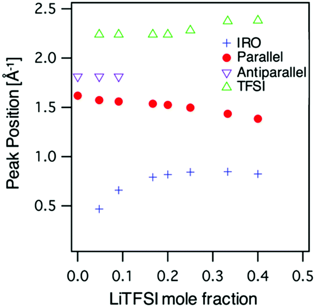Fig. 3 Peak positions as function of LiTFSI concentration from fits to the SAXS data, see text.

Fig. 4 Schematic of parallel and antiparallel nearest neighbour ordering in acetonitrile as proposed by Takamuku et al. in ref. 40, see text.

For the AN:LiTFSI electrolytes we focus first on the IRO peak at low Q. A systematic shift to higher Q with increasing salt concentration is observed until reaching a concentration of 5 AN per Li⁺ (5 : 1) whereafter the peak position remains around 0.8 Å⁻¹. Since the origin of the peak is due to the presence of Li⁺, we can envisage that the reordering of solvent molecules, as a result of Li⁺ solvation, is responsible for the changes observed in the SAXS data. This kind of intermediate range ordering, i.e., beyond the solvation shell, is atypical for organic solvent based electrolytes. However, the particular symmetry of the AN molecule could in principle allow for an extended ordering. As demonstrated by Takamuku et al. AN molecules tend to order in a parallel and antiparallel arrangement among first neighbours,⁴⁰ and this highlights that there can be a preferred alignment of AN. Furthermore, Sodeyama et al. also demonstrated, by means of molecular dynamics simulations, that AN molecules coordinated to Li⁺ are radially oriented.¹⁴ Based on the combined effects of these two observations, the induced radial orientation around Li⁺ and the ability of the AN molecules to align with each other will lead to the formation of an extended solvation shell around Li⁺, see Fig. 5. Thus, the presence of Li⁺ will induce a structuring of the AN molecules beyond the first solvation shell. With this picture in mind, we propose that the origin of the intermediate range order in AN/LiTFSI solutions arises from correlations between the solvation cluster of Li⁺.

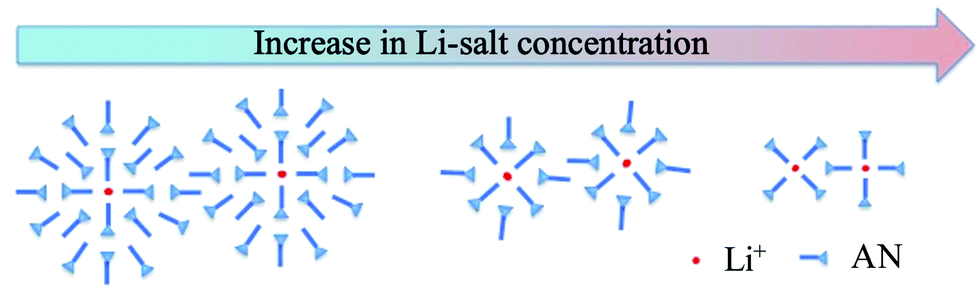Fig. 5 Schematic of solvation shells in the AN:LiTFSI solution as a function of Li-salt concentration. Note: The anion has not been taken into consideration.

To rationalise the scenario outlined above we can consider that in the most dilute solution (20 : 1) the position of the intermediate range order peak can be translated to an average real space distance around 13 Å. Identifying this distance as the distance between the Li-ions suggests that the extended solvation shell, or structuring of AN molecules, reaches out to 6–7 Å. As the concentration of LiTFSI is increased, the amount of AN molecules outside the first solvation shell, i.e., not directly coordinated to Li⁺, is reduced to allow for the solvation of the increased number of Li⁺. This effectively reduces the extended solvation shell, hence resulting in a shorter average distance between Li⁺. Upon reaching a ratio of 4 : 1, there is only enough AN molecules to form the first solvation shell, as AN is fourfold coordinated to lithium,⁴¹ thus the first solvation shells are in contact with each other. Therefore, any further increase in LiTFSI concentration does not result in a change in the position of the intermediate range order peak and we obtain a plateau value of ca. Q = 0.8 Å⁻¹. This is translated into a real space distance of 8 Å, which points to a size of the solvation shell around 4 Å, in good agreement with results from MD-simulations.¹⁴ So far, we have not explicitly considered the anion, TFSI, as part of the first solvation shell. At high Li-salt concentrations (e.g., 3 : 1 and 2 : 1) this becomes highly relevant since the number of AN molecules are too few to fully solvate the Li⁺. Hence, at the highest concentrations anions will be part of the first solvation shell⁴² and the intermediate range order will now resemble the charge ordering found in ionic liquids and solvated ionic liquids on the same length scales.^17,43 Based on a computational study Andersson et al. propose that at very high Li-salt concentrations a percolating network structure can be formed between coordinating clusters as a result of anions coordinating more than one Li-ion and that the 2 : 1 solution is just above the percolating threshold.²⁶ In this scenario the intermediate range order would represent a characteristic dimension of the percolating network. However, in our study we do not observe any significant changes in the SAXS data around the 2 : 1 concentration to support this picture. This can be due to a very weak signature of a percolation transition in SAXS, with characteristic distances actually barely changing, as well as that the percolation threshold differs slightly between the simulation and the experiment.

The ordering of AN molecules as a result of the introduction of Li-salt should also be reflected in the position of the nearest neighbour peaks of AN. The result from the fits of the SAXS data shows a decreasing intensity of the contribution from the antiparallel correlation, the peak at 1.6 Å⁻¹ in Fig. 3, and it can only be resolved up to concentration 10 : 1. This is reasonable since at concentrations of 5 : 1 and above no antiparallel configurations, which are second solvation shell correlations, are expected. In contrast the contribution from parallel configurations can be resolved for all concentrations and shows a weak decrease in the peak position with increasing salt concentration. To account for this behaviour, we can envisage two extreme scenarios in the electrolyte, AN molecules directly coordinated to Li⁺ and AN molecules in the extended solvation shell. The former are restricted to a radial configuration, which effectively results in larger distances between the AN molecules. The latter are allowed to have more relaxed orientations and can be more closely packed, similar to bulk like configurations in neat AN. Thus, the systematic decrease of the nearest neighbour peak position, i.e., an increased real space distance, as a function of LiTFSI concentration can be explained by a combination of these two extreme configurations.

The high Q-peak in the SAXS data evolves from a shoulder at the lowest concentration to a clear peak around 2.4 Å⁻¹ for the highest concentration. The position of the peak at high concentrations is within the typical range of intra-molecular correlations. Since the intensity of the peak scales with the increase in TFSI concentration, we believe that it is related to intra-ionic correlations of the anion. A corresponding peak can also be found in the structure factor of ionic liquids with the TFSI-anion and has been assigned to the partial structure factor of the anion.⁴⁴

3.2 Dynamics

With QENS we directly access the dynamics at the length scales of the features in the SAXS data at time scales around nano seconds. In the QENS experiment we use deuterated acetonitrile in order to avoid contribution from local relaxations, e.g., methyl group rotations, due to the strong scattering of hydrogen.

Fig. 6a shows results from an inelastic fixed window scan experiment on neat acetonitrile and electrolytes with concentrations 20 : 1, 5 : 1 (AN5) and 2 : 1 (AN2). In this experiment a peak is found in the intensity of inelastically scattered neutrons as a function of temperature, when the time scale of the dynamics in the material matches the time window of the spectrometer. From the data one can clearly see that only the time scale of the dynamics for the two higher concentrations matches the time window investigated on the IN16B spectrometer in this temperature range. The dynamics for lower concentrations are faster and the material needs to be cooled down to bring the dynamics into the spectrometer window. However, at these low temperatures both AN and the 20 : 1 solution crystallizes and could thus not be investigated. The strong shift of the peak position with temperature suggests a rather strong increase in the activation energy of the dynamical process contributing to the quasi-elastic scattering.

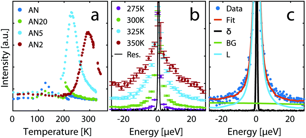Fig. 6 (a) Inelastic fixed window scans for neat AN and the solutions 20 : 1, 5 : 1, and 2 : 1. (b) QENS spectra at different temperatures for AN2 normalised to the value of the elastic peak. (c) Example of fit of a QENS spectrum to eqn (1) for AN2 at 300 K, Q = 1.4 Å⁻¹.

An example of raw data from the QENS experiment is shown in Fig. 6b. The broadening of the spectra implies that, as expected, there is increased dynamics as temperature is increased. To quantify the dynamics the data was fitted with

S(Q,ω) = R(Q,ω)⊗[A_E(Q)δ(ω) + A₁(Q)L₁(ω)] + BG (1)

where R(Q,ω) is the resolution function of the instrument, δ(ω) is the delta function to account for the elastic scattering, L₁(ω) is a Lorentzian function to model the quasi-elastic scattering, A_E(Q) and A₁(Q) are the areas of the delta and Lorentzian functions, respectively, and BG is a linear background (Fig. 6c).

From the fits the half-width at half maximum, Γ, of the quasi-elastic component can be extracted and it is related to the time scale of the motion. Fig. 7 shows Γ as a function of Q² and for a standard Fickian diffusion process Γ ∝ Q² is expected.⁴⁵ Our results shows a clear deviation from the Q²-dependence of Γ and bear instead the typical signature of a jump diffusion process.⁴⁵ Thus, to analyse the motion we fit the data with a jump diffusion model,⁴⁶eqn (2), where τ is the residence time between jumps and L is the average jump length.

From the parameters obtained by the fits to the model a local diffusion coefficient can be calculated from⁴⁶The parameters obtained from fits to the jump-diffusion model are shown in Fig. 8a–c. The jump length is found to be basically temperature and concentration independent with a mean jump distance around 1.7 Å (Fig. 8b). This points towards that the same or a similar type of process is observed for both concentrations. The jump distance is rather short compared to the nearest neighbour distances, ∼4 Å, and we can envisage this as a rotation, or reconfiguration, of an AN molecule or TFSI anion in the solvation shell, which would correspond to a dissociation from a particular Li⁺.

Fig. 7 Width of the quasi-elastic component as a function of momentum transfer at different temperatures for (a) AN5 and (b) AN2. Dashed lines are fits to the jump diffusion model in eqn (2).

Fig. 8 (a) Residence time, (b) jump length and (c) diffusion coefficient obtained from the fits with the jump diffusion model, eqn (2), as a function of temperature. (d–f) Same data with temperature axis scaled by T_g.

The residence time shows a temperature dependence as well as an increase with salt concentration (Fig. 8a). This is in agreement with Seo et al. who, based on molecular dynamics simulation results, proposed that the residence time increases with salt concentration up to 700 ps for concentrations corresponding to AN5.²³ The same trend is seen in our study, however, the residence time found in our experiment is considerably shorter, apart from the lowest temperatures at the highest concentration. Faster processes are reported by Okoshi et al. where ligand exchanges in DME:NaFSI electrolytes are predicted to occur on time scales of 60–120 ps²⁰ and by Åvall et al. where the ligand exchange in an AN:LiPF₆ electrolyte is estimated to 10 ps, with a slight decrease in residence time with increased concentration.²⁵ A recent study by Andersson et al. investigated the lifetime of the configurations around Li⁺ in a 2 : 1 AN : LiTFSI solution and found that the majority of configurations lasted less than 1 ps, where the longest calculated life time was 2 ps.²⁶ The discrepancy between the different studies can to some extent be associated to different criteria in the definition of a solvation shell, but also points to the need of benchmarking with experimental data. The diffusion coefficients calculated from eqn (3) also show a decrease with increasing salt concentration (Fig. 8c). The values calculated from the neutron scattering data are of the same order as previously reported,⁴⁷ supporting a connection between the observed process in QENS and the macroscopic ion transport.

By scaling the temperature axis in Fig. 8a–c with the glass transition temperature, T_g (169 K and 199 K for AN2 and AN5, respectively), one can make a more direct comparison between the two concentrations, Fig. 8d–f. This reveals that the residence time indeed has much stronger temperature dependence at higher salt concentrations. The residence time for AN2 shows a strong non-Arrhenius behaviour and almost diverges well above T_g, whereas the residence time in AN5 shows a more moderate increase approaching T_g. This is also underlined by the strong shift to lower temperatures of the peak in the inelastic fixed window scans, Fig. 6a, which suggests a strong decrease of the apparent activation energy with increasing AN content. Also, a small, but discernible difference in the diffusion constant can be observed. This is further underlined when considering the behaviour of the conductivity, Fig. 9. The conductivity decreases with increasing Li-salt concentration and with a T_g scaled temperature axis we also here observe that the conductivities for the two concentrations do not overlap. The difference in the temperature dependence, observed through the T_g scaling, points to differences in the interactions between the two systems. The origin of this difference can be attributed to the increased number of TFSI anions in the solvation shell around the Li⁺ and the accompanying strong increase of ionic interactions in the system. The rapid increase in the residence time in this scenario can then be interpreted as that AN2 has more stable solvation shells and that we in the QENS experiment have a larger contribution from dynamics of the TFSI anion. It could also point to a temperature dependence of the structure of the solvation shell favouring Li–TFSI interactions at lower temperatures. The similarity in the behaviour of the micro- and macroscopic dynamics, i.e., jump diffusion and ionic conduction, as a function of salt concentration and temperature provides the link between the two processes and that the local jump diffusion is the first step in the macroscopic ion transport process and that it is highly dependent on the local solvation structure.

Fig. 9 Conductivity as a function of (a) inverse temperature and (b) temperature axis scaled with T_g, for the different electrolytes.

4. Conclusion

The local structure and dynamics of acetonitrile was studied as a function of LiTFSI concentration using SAXS and QENS. Our results show that the geometry of the solvent plays an important role in the development of intermediate range order in the electrolyte solution as a result of correlations between solvation clusters. The ability of AN to order in parallel and antiparallel configurations gives rise to intermediate range ordering even at low Li-salt concentrations. At high Li-salt concentrations the presence of charge alternation-like ordering is found in the system as also TFSI anions start to take part in the solvation.

From the QENS data we show that the local dynamics of the solution can be well described by a jump diffusion model. The jump length is consistent with a typical reorientation of solvent molecules, or anions, in or out of solvation shells of the Li-ions. The jump length shows no, or very small, concentration or temperature dependence which is in agreement with a rather constant size of the solvation shell of a Li-ion. The residence time on the other hand shows a temperature and concentration dependence. The pronounced difference in the temperature dependence between AN2 and AN5 points to a difference in the local interactions, which is in agreement with proposed increase in the number of anions in the solvation shell. The almost diverging residence time as a function of temperature for AN2 also points to a temperature dependent solvation structure. A very long residence time also suggests that the transport mechanism starts to have an increased contribution from vehicular transport of the solvation shell, in addition to ligand exchange at the highest salt concentration at low temperatures.

Conflicts of interest

There are no conflicts to declare.

Acknowledgements

This research was financially supported by the Swedish Foundation for Strategic Research (SSF) within the Swedish national graduate school in neutron scattering (SwedNess) grant number GSn15-0008.

References

1. S. Goriparti, E. Miele, F. De Angelis, E. Di Fabrizio, R. Proietti Zaccaria and C. Capiglia, J. Power Sources, 2014, 257, 421–443.
2. B. L. Ellis, K. T. Lee and L. F. Nazar, Chem. Mater., 2010, 22, 691–714.
3. Y. Yamada and A. Yamada, J. Electrochem. Soc., 2015, 162, A2406–A2423.
4. J. Y. Song, Y. Y. Wang and C. C. Wan, J. Power Sources, 1999, 77, 183–197.
5. S. S. Zhang, J. Power Sources, 2006, 162, 1379–1394.
6. J. Wang, Y. Yamada, K. Sodeyama, C. H. Chiang, Y. Tateyama and A. Yamada, Nat. Commun., 2016, 7, 12032.
7. M. Nie, D. P. Abraham, D. M. Seo, Y. Chen, A. Bose and B. L. Lucht, J. Phys. Chem. C, 2013, 117, 25381–25389.
8. K. Yoshida, M. Tsuchiya, N. Tachikawa, K. Dokko and M. Watanabe, J. Phys. Chem. C, 2011, 115, 18384–18394.
9. Y. Yamada, K. Furukawa, K. Sodeyama, K. Kikuchi, M. Yaegashi, Y. Tateyama and A. Yamada, J. Am. Chem. Soc., 2014, 136, 5039–5046.
10. Y. Yamada, M. Yaegashi, T. Abe and A. Yamada, Chem. Commun., 2013, 49, 11194–11196.
11. Y. Kameda, Y. Umebayashi, M. Takeuchi, M. A. Wahab, S. Fukuda, S. Ishiguro, M. Sasaki, Y. Amo and T. Usuki, J. Phys. Chem. B, 2007, 111, 6104–6109.
12. K. Ueno, K. Yoshida, M. Tsuchiya, N. Tachikawa, K. Dokko and M. Watanabe, J. Phys. Chem. B, 2012, 116, 11323–11331.
13. S. Seki, N. Serizawa, K. Takei, K. Dokko and M. Watanabe, J. Power Sources, 2013, 243, 323–327.
14. K. Sodeyama, Y. Yamada, K. Aikawa, A. Yamada and Y. Tateyama, J. Phys. Chem. C, 2014, 118, 14091–14097.
15. K. Ueno, J.-W. Park, A. Yamazaki, T. Mandai, N. Tachikawa, K. Dokko and M. Watanabe, J. Phys. Chem. C, 2013, 117, 20509–20516.
16. T. Tamura, K. Yoshida, T. Hachida, M. Tsuchiya, M. Nakamura, Y. Kazue, N. Tachikawa, K. Dokko and M. Watanabe, Chem. Lett., 2010, 39, 753–755.
17. L. Aguilera, S. Xiong, J. Scheers and A. Matic, J. Mol. Liq., 2015, 210, 238–242.
18. R. Amine, J. Liu, I. Acznik, T. Sheng, K. Lota, H. Sun, C.-J. Sun, K. Fic, X. Zuo, Y. Ren, D. A. EI-Hady, W. Alshitari, A. S. Al-Bogami, Z. Chen, K. Amine and G.-L. Xu, Adv. Energy Mater., 2020, 10, 2000901.
19. Y. Aihara, K. Sugimoto, W. S. Price and K. Hayamizu, J. Chem. Phys., 2000, 113, 1981–1991.
20. M. Okoshi, C.-P. Chou and H. Nakai, J. Phys. Chem. B, 2018, 122, 2600–2609.
21. O. Borodin, L. Suo, M. Gobet, X. Ren, F. Wang, A. Faraone, J. Peng, M. Olguin, M. Schroeder, M. S. Ding, E. Gobrogge, A. von Wald Cresce, S. Munoz, J. A. Dura, S. Greenbaum, C. Wang and K. Xu, ACS Nano, 2017, 11, 10462–10471.
22. K. Dokko, D. Watanabe, Y. Ugata, M. L. Thomas, S. Tsuzuki, W. Shinoda, K. Hashimoto, K. Ueno, Y. Umebayashi and M. Watanabe, J. Phys. Chem. B, 2018, 122, 10736–10745.
23. D. M. Seo, O. Borodin, D. Balogh, M. O’Connell, Q. Ly, S.-D. Han, S. Passerini and W. A. Henderson, J. Electrochem. Soc., 2013, 160, A1061–A1070.
24. Z.-K. Tang, J. S. Tse and L.-M. Liu, J. Phys. Chem. Lett., 2016, 7, 4795–4801.
25. G. Åvall and P. Johansson, J. Chem. Phys., 2020, 152, 234104.
26. R. Andersson, F. Årén, A. A. Franco and P. Johansson, J. Electrochem. Soc., 2020, 167, 537.
27. M. A. González, B. Aoun, D. L. Price, Z. Izaola, M. Russina, J. Ollivier and M.-L. Saboungi, AIP Conf. Proc., 2018, 1969, 20002.
28. C. J. Jafta, C. Bridges, L. Haupt, C. Do, P. Sippel, M. J. Cochran, S. Krohns, M. Ohl, A. Loidl, E. Mamontov, P. Lunkenheimer, S. Dai and X.-G. Sun, ChemSusChem, 2018, 11, 3512–3523.
29. F. Nemoto, M. Kofu, M. Nagao, K. Ohishi, S. Takata, J. Suzuki, T. Yamada, K. Shibata, T. Ueki, Y. Kitazawa, M. Watanabe and O. Yamamuro, J. Chem. Phys., 2018, 149, 54502.
30. M. Kofu, M. Tyagi, Y. Inamura, K. Miyazaki and O. Yamamuro, J. Chem. Phys., 2015, 143, 234502.
31. T. Burankova, J. F. Mora Cardozo, D. Rauber, A. Wildes and J. P. Embs, Sci. Rep., 2018, 8, 16400.
32. F. Lundin, H. W. Hansen, K. Adrjanowicz, B. Frick, D. Rauber, R. Hempelmann, O. Shebanova, K. Niss and A. Matic, J. Phys. Chem. B, 2021, 125, 2719–2728.
33. J. Zheng, J. A. Lochala, A. Kwok, Z. D. Deng and J. Xiao, Adv. Sci., 2017, 4, 1700032.
34. R. Tatara, Y. Yu, P. Karayaylali, A. K. Chan, Y. Zhang, R. Jung, F. Maglia, L. Giordano and Y. Shao-Horn, ACS Appl. Mater. Interfaces, 2019, 11, 34973–34988.
35. K. Qian, R. E. Winans and T. Li, Adv. Energy Mater., 2021, 11, 2002821.
36. H. W. Hansen, M. Appel, B. Frick, F. Lundin, A. Matic and J. Rizell, Institut Laue-Langevin (ILL), 2018,  DOI:10.5291/ILL-DATA.6-02-589.
37. B. Frick, J. Combet and L. Van Eijck, Nucl. Instrum. Methods Phys. Res., Sect. A, 2012, 669, 7–13.
38. D. Richard, M. Ferrand and G. J. Kearley, J. Neutron Res., 1996, 4, 33–39.
39. R. T. Azuah, L. R. Kneller, Y. Qiu, P. L. W. Tregenna-Piggott, C. M. Brown, J. R. D. Copley and R. M. Dimeo, J. Res. Natl. Inst. Stand. Technol., 2009, 114, 341–358.
40. T. Takamuku, M. Tabata, A. Yamaguchi, J. Nishimoto, M. Kumamoto, H. Wakita and T. Yamaguchi, J. Phys. Chem. B, 1998, 102, 8880–8888.
41. D. M. Seo, P. D. Boyle, O. Borodin and W. A. Henderson, RSC Adv., 2012, 2, 8014–8019.
42. E. Flores, G. Åvall, S. Jeschke and P. Johansson, Electrochim. Acta, 2017, 233, 134–141.
43. L. Aguilera, J. Völkner, A. Labrador and A. Matic, Phys. Chem. Chem. Phys., 2015, 17, 27082–27087.
44. H. K. Kashyap, C. S. Santos, H. V. R. Annapureddy, N. S. Murthy, C. J. Margulis and E. W. Castner Jr, Faraday Discuss., 2012, 154, 133–143.
45. M. Bee, Quasielastic neutron scattering, Adam Hilger, United Kingdom, 1988.
46. J. Teixeira, M.-C. Bellissent-Funel, S. H. Chen and A. J. Dianoux, Phys. Rev. A: At., Mol., Opt. Phys., 1985, 31, 1913–1917.
47. J. Zhang, R. E. Corman, J. K. Schuh, R. H. Ewoldt, I. A. Shkrob and L. Zhang, J. Phys. Chem. C, 2018, 122, 8159–8172.

---