
 Open Access Article
 This Open Access Article is licensed under a
 Creative Commons Attribution 3.0 Unported Licence
Designing excitonic circuits for the Deutsch–Jozsa algorithm: mitigating fidelity loss by merging gate operations†
Maria A.
Castellanos
and
Adam P.
Willard
 *
*
Department of Chemistry, Massachusetts Institute of Technology, Cambridge, MA, USA. E-mail: awillard@mit.edu
First published on 21st June 2021
Abstract
In this manuscript, we examine design strategies for the development of excitonic circuits that are capable of performing simple 2-qubit multi-step quantum algorithms. Specifically, we compare two different strategies for designing dye-based systems that prescribe exciton evolution encoding a particular quantum algorithm. A serial strategy implements the computation as a step-by-step series of circuits, with each carrying out a single operation of the quantum algorithm, and a combined strategy implements the entire computation in a single circuit. We apply these two approaches to the well-studied Deutsch–Jozsa algorithm and evaluate circuit fidelity in an idealized system under a model harmonic bath, and also for a bath that is parameterized to reflect the thermal fluctuations of an explicit molecular environment. We find that the combined strategy tends to yield higher fidelity and that the harmonic bath approximation leads to lower fidelity than a model molecular bath. These results imply that the programming of excitonic circuits for quantum computation should favor hard-coded modules that incorporate multiple algorithmic steps and should represent the molecular nature of the circuit environment.
1 Introduction
Excitonic circuits comprised of precisely arranged sets of electronically coupled dye molecules can be designed to manipulate the evolution of an exciton wavefunction so that it performs elementary quantum computations.1 The ability to design these circuits for specific computations and optimize them for improved fidelity and synthetic convenience is key to the development of quantum technologies based on the circuits. However, circuit optimization is complicated due to ambiguity in design strategy, because there are generally numerous different circuit geometries capable of performing a given computation. In this manuscript, we compare two different strategies for designing excitonic circuits that carry out a simple 2-qubit algorithm, with the goal of exploring how suitable these systems are for rudimentary quantum information applications. We find that the strategy of hard-coding the entire algorithm into a single circuit has potential to yield significantly higher fidelity than a modular strategy, for which the algorithm is implemented as a sequence of universal quantum gate operations. This finding thus exposes significant practical barriers to the scalability and programmability of excitonic circuits for more complicated quantum algorithms.An excitonic circuit is a network of moieties – typically, organic chromophores – that are each capable of supporting an exciton, i.e., a coulombically bound excited electron–hole pair. The network of couplings between these moieties determines the delocalization and dynamics of the exciton wavefunction and can thus potentially be tailored to control certain aspects of exciton dynamics. The ubiquitous example from biology is in photosynthesis, where excitonic circuits have evolved to mediate the efficient transfer of photon energy to reaction centers.2–4 Excitonic circuits also have been synthesized by positioning dye molecules in rigid scaffolds of DNA5–8 or proteins.9,10 By enabling nanoscale control of energy flow, excitonic circuits have the potential to play a role in the development of novel molecular scale electronic technologies.
One potential application of excitonic circuitry is quantum computing. Excitons carry information about quantum phase, coherence, and entanglement that can be systematically manipulated within appropriately designed systems.8,11–14 These quantum dynamical properties can be tuned to encode specific quantum transformations, or sequences of transformations. In previous work, we demonstrated the design of excitonic circuits for the universal quantum gate operations.1 Here, we extend this work to the design of a simple multi-step 2-qubit quantum algorithm – the 2-qubit Deutsch–Jozsa algorithm – where there are multiple approaches to circuit design. Our results highlight that computational fidelity can depend significantly on the chosen design strategy.
By leveraging properties of coherence and entanglement, quantum computing has the potential to dramatically out-perform classical computing in certain important tasks such as cryptography, quantum search, quantum simulation and quantum walks.15–19 Any quantum computation can be expressed as a sequence of individual gate operations (e.g., NOT, π/8, HADAMARD, CNOT) carried out on a array of input qubits.20,21 Qubits can be constructed from two-state quantum systems, such as spin-1/2 particles or nuclei. Gate operations, which transform the state of these systems by manipulating phase and creating superpositions or entanglements, can be expressed as unitary operators acting on one or more qubits. An operation carried out on a register of n qubits can thus be formalized as a 2n × 2n unitary operator transforming an input qubit array to an output qubit array.
In our approach, the state of a qubit array is indicated by the occupation state of an exciton in a system of multiple separate dye molecules. For instance, a single qubit is described by an exciton in a system of two dye molecules (A and B), with the 0 or 1 qubit states corresponding to the exciton fully localized on molecule A or molecule B, respectively. We encode the unitary operations acting over a qubit state in the time evolution of the system Hamiltonian, controlling the coupling through precise geometric positioning of the dye molecules, as described in more detail in ref. 1 and summarized in Section 3.1 below. The evolution of an exciton within a specifically designed system of dye molecules over a particular time interval therefore corresponds to the change in state of the associated qubit array.
In the next section, we review the Deutsch–Jozsa algorithm. Then, in Section 3, we describe how this algorithm can be implemented with excitonic circuits. We present excitonic circuits based on two different design strategies – serial and combined – and in Section 4 we evaluate the fidelity of these hypothetical circuits under the influence of a harmonic bath. In Section 5 we propose a specific atomistic realization of these circuits and evaluate their performance with a more realistic bath model. Finally, in Section 6 we conclude by discussing the practical implications of our results in the context of more complicated quantum computations.
2 The Deutsch–Jozsa algorithm
The Deutsch–Jozsa (D–J) algorithm is one of the simplest algorithms for which a quantum computer outperforms a classical one.22 The algorithm distinguishes the identity of a black-box ‘oracle gate’ that transforms an input binary array of n bits, e.g., (0,1,1,0,…,1) to a single binary output value, i.e., 0 or 1. The two possible identities of this oracle gate are ‘constant’, in which the output is always the same (i.e., always 1 or always 0, regardless of the input), and ‘balanced’, in which the output is 0 for half of the input states and 1 for the other half. To unambiguously determine the identity of an unknown oracle gate requires multiple queries with classical computation (at least 2n−1 + 1), but only requires a single query with quantum computation.23 This algorithm has been implemented in several physical systems, such as nuclear spins,24 ion traps,25 and superconductors26 as a way to demonstrate their feasibility as potential quantum computing platforms.
Fig. 1A depicts the quantum circuit diagram for identifying a n = 1 oracle gate, f. The quantum algorithm, which requires two qubits, involves performing Hadamard operations carried out on one or both qubits after and before evaluating the oracle gate, respectively. Specifically, the first set of Hadamard operations transform the input state, |Ψ〉i = |0〉|1〉 into a superposition state, i.e., |Ψ〉1 = |+〉|−〉, where  . The action of the oracle gate is to perform a phase kick-back operation on the second qubit, Uf: |x〉|y〉 → |x〉|y ⊕ f(x)〉 = (−1)f(x)|x〉|y〉. When N = 2, f(x) can take 1 of 4 possible values: f(x) = 0 or f(x) = 1, when constant, and f(x) = x or f(x) = NOTx, when balanced. After the third step, the final state of the qubit register will then be |Ψ〉F = ±|0〉|−〉 or |Ψ〉F = ±|1〉|−〉 if the oracle gate is constant or balanced, respectively. A single measurement over the ancilla qubit (i.e. qubit 1) at the conclusion of the algorithm therefore reveals the identity of the “black box” oracle function.
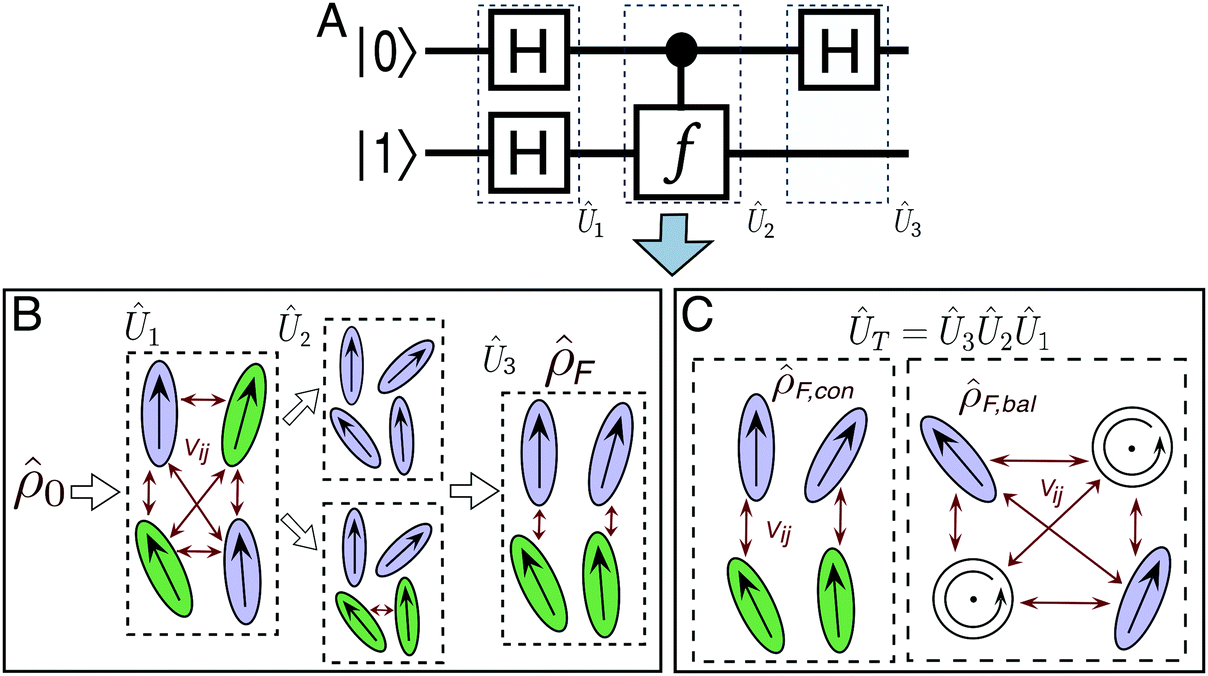 | ||
| Fig. 1 (A) Quantum circuit diagram representing the Deutsch–Jozsa algorithm. (B) Schematic representation of the 2-qubit excitonic circuit geometry for the serial strategy. This circuit transforms an input exciton state, ρ0, into an output state, ρF, via three steps. Dye molecules are represented by ovals and the molecular species is indicated by shading. Non-zero coupling is indicated by red arrows. The top and bottom branches in the middle step correspond to the constant and balanced cases, respectively. (C) Schematic excitonic circuit geometry for the combined strategy for the constant (left) and balanced (right) algorithms. The balanced algorithm includes dye molecules (circles) that are excited via circularly polarized photons. | ||
3 Implementing the Deutsch–Jozsa algorithm with excitonic circuits
In this section we describe two general strategies for representing a simple quantum algorithm as an excitonic circuit of precisely arranged dye molecules. The first is a serial strategy, where each quantum gate operation is carried out sequentially. The second is a combined strategy, where the entire algorithm is carried out by a single circuit.3.1 Mapping the D–J algorithm onto the Frenkel Hamiltonian
We propose excitonic circuits for the D–J algorithm following the procedure described in ref. 1. Our approach to excitonic circuit design for an n-qubit quantum computation maps the N × N unitary operator for the computation, where N = 2n, to the Frenkel Hamiltonian of a system of N dye molecules. This mapping is given by,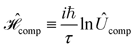 | (1) |
 is the corresponding Frenkel Hamiltonian. When the system defined by
  , i.e., a single exciton on N dye molecules, is evolved for time τ, the change in the exciton wavefunction thus encodes the result of the computation defined by Ûcomp. The design of an excitonic circuit for a given quantum computation therefore involves specifying the identities and relative positions of dye molecules that yield a Hamiltonian equivalent to
  .
.
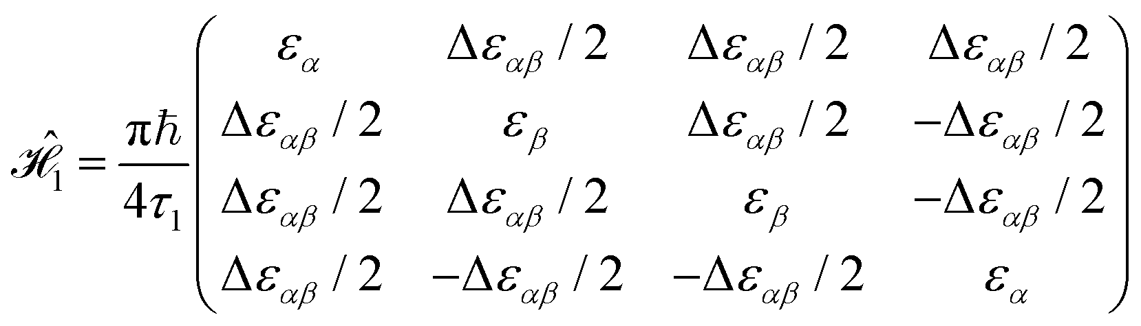
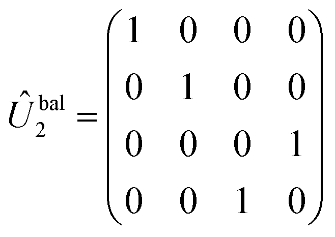
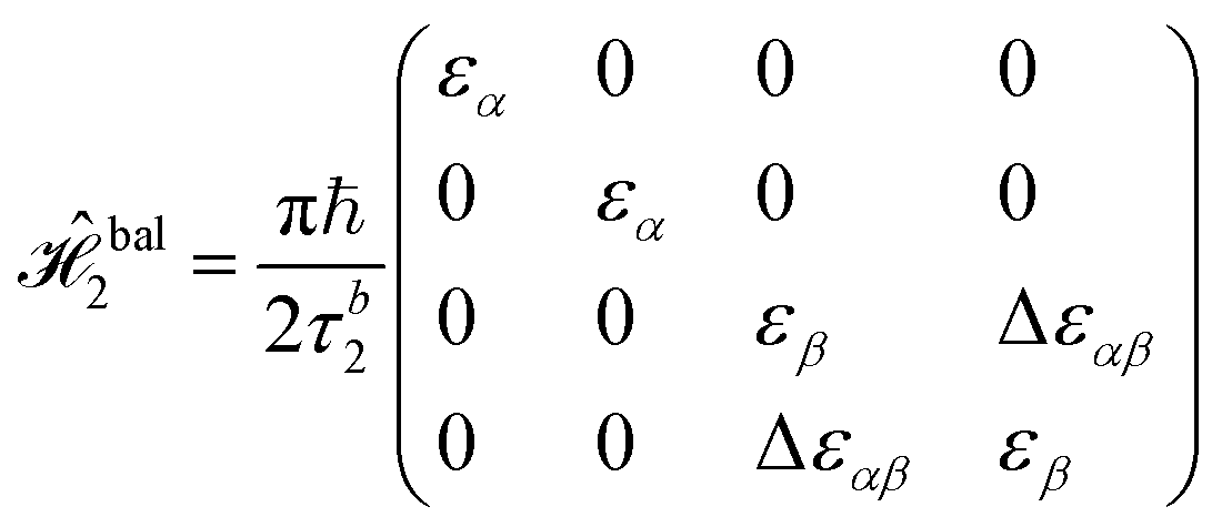
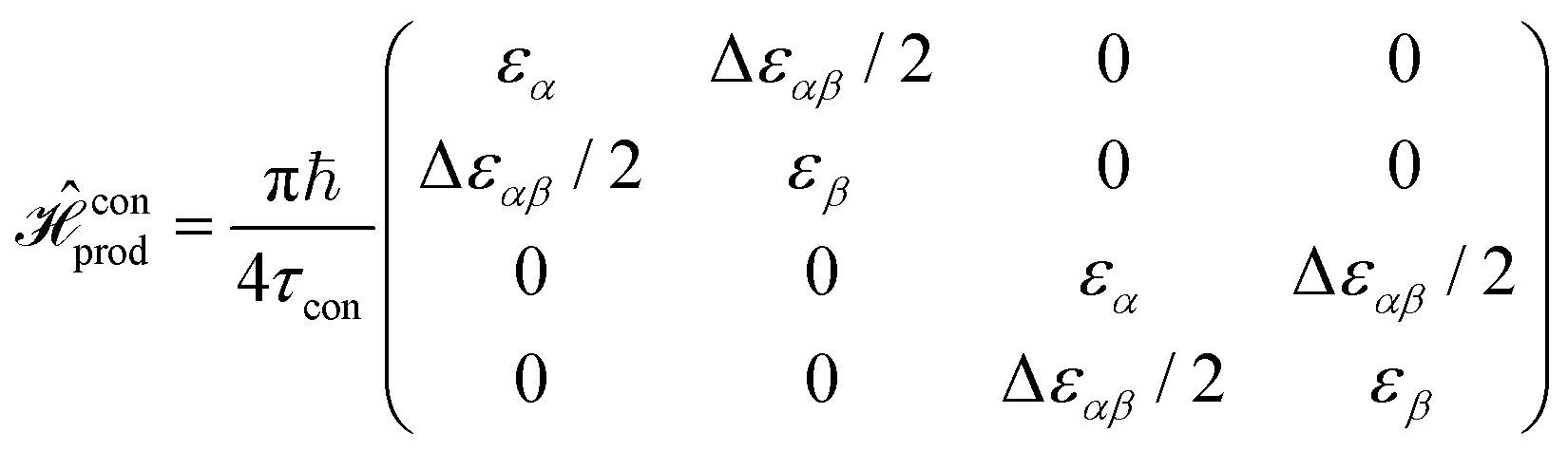
There are many possible strategies for designing an excitonic circuit for the multi-step D–J algorithm. For instance, the algorithm can be equivalently represented by either a sequence of three 2-qubit unitary operations (i.e., Û1, then Û2, then Û3), one for each step in the circuit diagram of Fig. 1A, or a single unitary operation that combines all three steps (i.e., Ûprod = Û3Û2Û1). These two limiting strategies, as illustrated in Fig. 1B and C, yield either four distinct circuits in the serial case (one for each of the first and third steps and one for each of the balanced and constant oracle gates) or two distinct circuits in the combined case (one for the balanced case and one for the constant case). The unitary operators and corresponding system Frenkel Hamiltonians for the serial and combined strategies of excitonic circuit design are contained in Table 1, as derived from eqn (1).
| Operation | Unitary operator | Hamiltonian |
|---|---|---|
| First step |

|
|
| Oracle |

|

|
|
|
|
| Third step |
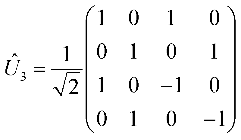
|

|
| Combined, constant |

|
|
| Combined, balanced |

|

|
 , which is then evolved for time τ1 and transferred to another system described by
  . This exciton is then evolved for time τ2 and transferred to a third system described by
  . The exciton is then allowed to evolve for time τ3 on system 3 before it is read out. Experimentally, a particular initial state can be created by laser excitation of the ground state of a specific dye or a combination of dyes. While the exciton state in the last step can be detected through photon emission. Specifically, the final state of an exciton after coherent manipulations can be detected from single-photon spontaneous emissions.27 On the other hand, an excitation can be transferred between two organic circuits using Förster Resonance Energy Transfer (FRET).28 However, there exist no robust implementation that can manage to transfer the state of the exciton precisely between two circuits, at least without previous knowledge of the instantaneous state at τi. Furthermore, because initialization and detection in the present system cannot occur without errors, the proposed serial circuit is purely hypothetical and its fidelity can only represent an upper bound on the system if implemented in practice. Therefore, for the sake of systematically isolating the effects of circuit design, we neglect fidelity loss from initialization, exciton transfer, and detection, assuming they all occur without error and with 100% fidelity.
The form of the Frenkel Hamiltonians for each step of the D–J implies the relative excitation energies and positions of a set of four dye molecules (A, B, C, and D). The excitonic circuit implied by  (Table 1) corresponds to two pairs of homodimers that are all coupled with equivalent magnitudes as determined by the excitation energy difference between the two dye species. The coupling leads to delocalization in the exciton basis and a corresponding superposition state in the qubit basis. Differences in excitation energy between the dye molecules leads to the accumulation of a relative phase shift over time τ1.
The excitonic circuits implied by  and
and  are straightforward to interpret. The constant operation corresponds to an identity matrix, and therefore is implied by a circuit of 4 identical and uncoupled dyes and an arbitrary value of τ. On the other hand,
  (equivalent to a CNOT operation) is represented by two different pairs of homodimers, one uncoupled and one coupled.
The excitonic circuit implied by  is an uncoupled pair of identical coupled heterodimers (Fig. 1). This system concentrates the delocalized exciton population in one of two entangled states, depending on the output state of the exciton from the constant or balanced oracle circuit. Specifically, over time τ3 the population is funneled into one pair of dyes (A and B) if the oracle function is constant, or into the other (C and D) if it is balanced.
 is an uncoupled pair of coupled heterodimers. Notably, this circuit is effectively identical to that of the circuit for
  . This similarity implies that the specific operation of the constant oracle operator is essentially trivial and simply drops out of the combined unitary operator, leading to a significant simplification of the resulting excitonic circuit.
Finally, implies a circuit of two pairs of homodimers, with all dyes coupled to each other. Notably, the system features imaginary-valued couplings. Imaginary coupling can occur between two dyes if each one is electronically excited using a different polarization of light. For example, if one dye is initialized using linearly polarized light with unequal x–y amplitudes and the other dye is excited with circularly polarized light. This arrangement can be achieved, for instance, with a metalloporphyrin and cyanine dye pair. Circularly polarized light can induce a directional electronic current in the porphyrin ring, that results in the formation of a degenerate complex excitation,29 and to a complex-valued molecular coupling upon interaction with a real non-degenerate excitation from the cyananine pair.
4 Simulating the performance of idealized excitonic circuits in model environments
The Hamiltonians in Table 1 represent idealized systems that in the absence of an environment (i.e., a closed quantum system) will perform the given computation in time τ with unit fidelity. However, any practical application will include the influence of a noisy environment. In this case, system–bath interactions lead to dephasing and dissipation that can alter the output and thus degrade fidelity.In this section we simulate the influence of a model environment on the fidelity of idealized D–J excitonic circuits. We compare overall fidelity loss between idealized serial and combined circuits. We assume that serial circuits lose no fidelity between steps. Because fidelity losses due to dissipation are expected to be negligible on the timescales of interest, we only consider the effect of dephasing in the system dynamics. We also assume that the input state of the wavefunction can be precisely prepared and the output state can be precisely detected at time τ. With these assumptions, we can evaluate fundamental differences in fidelity between circuits designed with the serial and combined strategies. We describe the state of the excitonic wavefunction in terms of a reduced density matrix and simulate the evolution of that wavefunction using a Redfield master equation under the secular approximation.30,31 We describe the system using a simple system–bath Hamiltonian,
 | (2) |
 is the Frenkel Hamiltonian of one of the excitonic circuits in Table 1,
  describes the thermal bath and
  describes the system–bath coupling. We model the bath as a collection of N (i.e., one for each dye molecule) independent harmonic oscillators,
 | (3) |
 | (4) |
 | (5) |
 | (6) |
 | (7) |
We choose bath parameters to model a condensed phase chromophoric system at 300 K. Specifically, following ref. 33, we set λ = 100 cm−1 ≈ 0.012 eV and Ωc to be proportional to λ by 2λ/(βΩc2) = 1.2.34 The dephasing time, tD = 1/γ, was chosen to be (3/4)τ for all dyes in a given circuit, where τ is the transformation time for the mapped operation. We parameterize the dye molecules in our circuit based on Cy3–oxypropyl and Cy5–oxypropyl molecules. Specifically, we always assume that dye A is a Cy3 species with excitation energy εα = 3.24 eV. In circuits that require two dye species (i.e., A and B), we assume the B dye species is Cy5 with εβ = 2.85 eV. These values reflect the first excited state energies as computed from time-dependent density functional theory (TDDFT) with a 6-31G+(d) basis and WB97XD DFT functional.
The resulting dynamics for the four studied systems, namely, the serial and combined excitonic circuits, both for the constant and balanced versions of the algorithm, are shown in Fig. 2. The influence of system–bath interactions on the fidelity of a given computation is encoded in the structure and evolution of the reduced density matrix, ![[small rho, Greek, circumflex]](https://www.rsc.org/images/entities/i_char_e0b7.gif) . This influence can be illustrated by tracking a single element of in both a closed and open system. In Fig. 2A, we plot the exciton population on dye C throughout the sequence of transformations described for the serial D–J algorithm in its constant version, namely
. This influence can be illustrated by tracking a single element of in both a closed and open system. In Fig. 2A, we plot the exciton population on dye C throughout the sequence of transformations described for the serial D–J algorithm in its constant version, namely  ,
,  and
and  , while Fig. 2B depicts the dynamics for the balanced version. We focus on this dye molecule because its final population indicates the identity of the oracle gate. Moreover, these populations are presented as segmented plots, in order to illustrate how the populations are transferred sequentially thorough the algorithm, at each transformation time. The full population dynamics for the individual circuits can be found in Fig. S1 (ESI†).
 | ||
| Fig. 2 Time-evolution of the populations of the D–J algorithm with a model environment. The population for the Cy3(C) dye as the wavefunction evolves through the first, second and last step, for (A) the constant and (B) balanced version. The segmented dynamics illustrate the transference of populations to subsequent steps, when the transformation time is reached (vertical dotted lines). The populations for all four dyes for the single-step in the combined approach, for (C) the constant and (D) the balanced version. Here, τ is indicated with a black dotted line. The populations for the closed system are shown in dashed lines on each plot. For the combined constant version, note that 22 and 33 are both constant in zero. | ||
Phase loss in the open system (solid lines in Fig. 2) results in a decrease in fidelity that grows with time. In the serial system, shown in Fig. 2A and B, phase loss accumulates with each subsequent step. It can be seen that dephasing is most significant in the final step of the algorithm in both serial systems. Indeed, the details of the system Hamiltonian set the dephasing rates for each different excitonic circuit.
In contrast, the combined systems, shown in Fig. 2C and D, require only a single step. In the constant system (Fig. 2C) the system maintains high fidelity despite being prone to dephasing due to the short computation time, τcon ≈ 4 fs. Notably, the balanced system requires a much longer computation time (τbal ≈ 13 fs) yet features negligible fidelity loss. This observation implies that some circuits retain fidelity much better than others and that design efforts may require a trade-off between circuit complexity and fidelity retention.
In order to quantify how much of the information contained in the final quantum state is lost due to fluctuations in the bath, we define the fidelity of the open quantum state,
 | (8) |
(cl)(t), and that of the open system under pre-defined environmental conditions, (op)(t). To account for uncertainty in the measurement associated with any possible experimental set-up to be used to read the final state, we assume (op) cannot possibly be measured exactly at t and, thus, we randomly choose a time tm from the range tm ∈ {t − Δt,t + Δt}, where Δt is the uncertainty in the measurement (here chosen to be Δt = 0.2 fs), and average over the total number of observations, M: | (9) |
We use this equation to compute the fidelity of the open D–J excitonic circuits. Under a serial approach, the fidelity decreases as ![[F with combining macron]](https://www.rsc.org/images/entities/i_char_0046_0304.gif) (τ1) = 0.93 → (τc2) = 0.74 → (τ3) = 0.65 (with τc2 set to 2 fs), and (τ1) = 0.93 → (τb2) = 0.79 → (τ3) = 0.69, from the first to third step of the algorithm, for the constant and balanced D–J, respectively. That is, the fidelity decreases consistently with each step, such that there is significant uncertainty in the identity of the oracle function upon measurement on the state 3(τ). On the other hand, the calculated fidelities for the combined approach are significantly higher, (τcon) = 0.96 and (τbal) = 0.97. Notably, the lower fidelities of the serial circuits do not include the effects of fidelity loss in the transfer of excitons from one circuit to the next. We thus speculate that the combined strategy for excitonic circuit design yields calculations with much higher fidelity than a serial strategy.
(τ1) = 0.93 → (τc2) = 0.74 → (τ3) = 0.65 (with τc2 set to 2 fs), and (τ1) = 0.93 → (τb2) = 0.79 → (τ3) = 0.69, from the first to third step of the algorithm, for the constant and balanced D–J, respectively. That is, the fidelity decreases consistently with each step, such that there is significant uncertainty in the identity of the oracle function upon measurement on the state 3(τ). On the other hand, the calculated fidelities for the combined approach are significantly higher, (τcon) = 0.96 and (τbal) = 0.97. Notably, the lower fidelities of the serial circuits do not include the effects of fidelity loss in the transfer of excitons from one circuit to the next. We thus speculate that the combined strategy for excitonic circuit design yields calculations with much higher fidelity than a serial strategy.
The difference in fidelity between the two strategies can be observed more clearly by comparing as a function of time for the combined and serial approach, as shown in Fig. 3. These results highlight that fidelity loss rates differ between steps in the serial circuits and that certain steps can dominate overall fidelity loss. For both cases considered here, the second step (associated with the action of the oracle gates) is the most significant source of fidelity loss. These results also highlight that fidelity loss rates are significantly lower for the combined strategy than for the serial strategy. These differences reflect the benefit of lowering the total computational time, thereby reducing system–bath interactions, but also reveal that some circuits are fundamentally better at retaining exciton phase information than others.
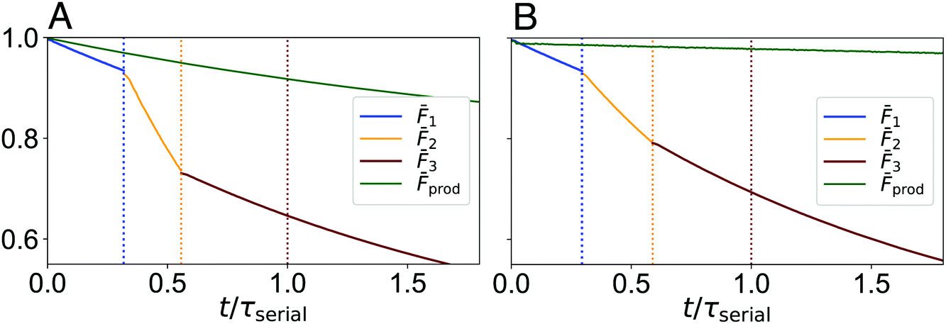 | ||
| Fig. 3 Fidelity of the serial and combined approaches as a function of time, for (A) the constant and (B) balanced circuits, respectively. Transformation times τ1, τ1 + τ2 and τ1 + τ2 + τ3 = τserial are indicated by blue, orange and red dotted lines, respectively. In both panels, the time axis is scaled to the total computational time of the serial approach. For the constant case τserial = 8.4 fs and τprod = 3.7 fs. For the balanced case τserial = 9.0 fs and τprod = 13.0 fs. | ||
5 Designing explicit molecular representations of excitonic circuits
The systems implied by the idealized Hamiltonians of Table 1 are hypothetical in that they ignore the potential for steric clashes and geometric frustration that may arise in a physical multi-dye system. Thus, in this section we construct D–J excitonic circuits by arranging four explicit dye molecules in space and we evaluate the performance of the resulting circuits.We design an excitonic circuit constructed from all-atom representations of Cy3 and Cy5 dyes. Cyanine dyes are often used in synthetic dye-based systems due to their photostability, high fluorescence efficiency, low Stokes shift, commercial availability, and compatibility with common experimental set-ups.7,35 Cyanine dyes provide a simple platform to assess the potential effect of noisy environments in quantum operations encoded in excitonic circuits. Moreover, the electronic coupling within Cy3 dye pairs has been demonstrated to be tunable when these dyes are scaffolded in DNA.36 We expect that a similar analysis can be carried out in other exciton molecular systems, perhaps less prone to noise than the constructs we employ here.
We narrow our focus to the constant version of the D–J algorithm, noting that qualitative differences in fidelity between the combined and serial approaches are expected to hold in general. This choice provides simplicity in both the form of the Hamiltonian for the constant oracle operator, a scaled identity operator, and the fact that  and
and  are isomorphic and can thus be carried out on identical circuits.
Our approach is to first identify a geometric arrangement of dye molecules whose interactions approximate a target Frenkel Hamiltonian. We then apply soft constraints to these dye molecules and simulate their dynamics in explicit solvent, using electronic structure calculations to compute bath parameters. With these parameters and the approximate Hamiltonian, we simulate the evolution of the reduced density matrix and analyze the associated computational Fidelity.
The resulting Hamiltonian evolution is thus a preliminary assessment on the viability of excitonic circuits for the implementation of quantum algorithms, that can more accurately describe the expected fidelity than the model description in Section 4.
5.1 Genetic algorithm for the design of excitonic circuits
In this subsection we describe the development of a genetic algorithm for positioning atomistic representations of dye molecules to yield specific target electronic coupling values. In principle, it is possible to realize these spatial representations by scaffolding the cyanine dyes in macromolecular scaffoldings, although a significant level of error is expected. The method presented here is intended to be a guide as to how to translate the systems described in Section 3 into more realistic molecular representations.As determined by the Hamiltonians in Table 1 and illustrated in Fig. 1, the circuits we aim to create contain two species of dye molecules differing in their excitation energies. The specific dyes that are chosen will set the value of ε1 and ε2 and therefore determine the magnitude of coupling that is required to enable the computation (i.e., off-diagonal elements in  ). Coupling is a sensitive function of intermolecular separation and orientation so there are, in principle, numerous arrangements of a dye pair that will yield the same coupling value. However, identifying the positioning of a multi-dye system that simultaneously satisfy multiple couplings can be a difficult task.
We undertake this task by performing a search of dye positioning that is biased to favor configurations with a specific set of intermolecular coupling values. For any specific configuration, we compute each value of the intermolecular electronic coupling in an atomistic basis via the point monopole approximation, which has been demonstrated to accurately represent couplings between closely spaced organic dye molecules.37,38 Specifically, we define the coupling between molecules i and j as,
 | (10) |
Identifying configurations of a 4-dye system described by a given  requires simultaneously satisfying up to six coupling values. We search for these configurations via a genetic algorithm (GA) as follows: for a given set of dyes (e.g., two pairs of Cy3 and Cy5 dyes) the position of one of the molecules is fixed (e.g., dye A), while the positions of the remaining dyes (e.g., dyes B, C and D) are varied. The GA is designed to find the optimal arrangement of the 3 mobile dyes coordinates such that the system's coupling resembles that of the desired Hamiltonian. Specifically, given the system is initialized such that the center of mass of all 4 molecules is located at the origin, the coordinates of dyes B, C and D are modified by a series of translation-rotation operations of the form,
| (xf,yf,zf) = Rx(θx)Ry(θy)Rz(θz)[(x0,y0,z0) + (dx,dy,dz)], | (11) |
 , with the desired one,
  (from Table 1),
 | (12) |
We carry out the GA until the fitness function in eqn (12) has been maximized.
For the  circuit, the genes comprise the possible rotation and translation operations of eqn (11), keeping one of the Cy3 dyes fixed and imposing a steric constraint that the atoms of any pair of dye molecules be separated by more than 2 Å. The GA was run until convergence over a configuration space that includes all dye displacements within a sphere in which Vij ≠ 0, and with all dye rotation angles ranging from −π/2 to π/2. Due to the steric constraint and the need for large coupling values (V ≈ 0.1–0.2 eV), there is no guarantee of finding a nearly exact solution with this approach. Fig. 4B depicts the geometry calculated with this method, which has a fitness of Γ = 75%, and a calculated fidelity of = 82.3%.
 | ||
Fig. 4 Schematic of the dye circuits representing the DJ algorithm and corresponding Hamiltonians. (A) For the excitonic circuit found to evolve similarly to  , and whose spatial distribution was determined using GA, and (B) for the circuit evolving as , and whose spatial distribution was determined using GA, and (B) for the circuit evolving as  (and (and  ). ). | ||
Finding an optimal geometry for  following this recipe is a simple problem, since only a single coupling must be satisfied. Here, only the Cy3–Cy5 pairs will be coupled, and the coupling between the two possible pairs is exactly the same. In fact, due to this simplicity, the circuit can be optimized without the use of the GA. Fig. 4A shows the resulting geometric configuration for
  , calculated using the described method. This geometry yields a value of Γ = 99.5%.
5.2 Simulation methodology
In this subsection, we outline the process for characterizing the system–bath interaction on an explicit dye system. Once the optimal geometry for a specific transformation Hamiltonian is identified, a series of classical and ab initio calculations can be carried out to describe the effect of the bath fluctuations on the system dynamics. This effect can be fully described in terms of the excitation energy autocorrelation function. In the present model only the first excited state is accessible, and therefore the autocorrelation function is calculated for the energy gap from the ground to excited state, ε01. To compute the correlation function, we first use classical MD to generate ground state equilibrium dynamics of the dye system immersed in bulk liquid water at 300 K. We then compute the excited state energy, ε01 for each dye separately at each step of the MD simulation.40–43 Finally, we calculate the correlation function, | (13) |
 denotes the ith discrete MD timestep, Nt is the total number of steps in the trajectory, t = δt × i, and δt = 4 fs is the timestep increment in the MD simulations.
We assume each molecule is interacting with its own local bath. Under the Kubo stochastic lineshape theory, the dephasing function, characterizing the exponential decay on the system's phase, can be calculated from the energy gap correlation function,44
 | (14) |
The dephasing time can likewise be calculated from integration over the dephasing function, D(t),
 | (15) |
Therefore, following a similar argument as in Section 4, eqn (14) and (15) can be used to describe the system operator, Gm, for each one of the four dyes in the circuit, with γD = 1/tD. Similarly, the energy gap correlation function, C(t), can also be used to derived the frequency-dependent bath contribution to the interaction  , contained in the spectral density, J(ω). We use the following definition,
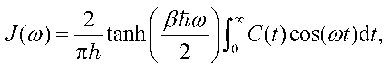 | (16) |
 is often used to describe these modes.
The variation in the energy gap, ε01(ti), was estimated along multiple trajectories. In total two sets of simulations were carried out, one for the first step of the D–J algorithm and one for the third step. Each trajectory was generated through a MD simulation on each system, composed of two Cy3–oxypropyl and two Cy5–oxypropyl dyes. The Generalized Amber Force Field (GAFF)46 was employed to describe the cyanine molecules, and their respective atomic point charges were generated with a RESP fit, using the Q-Chem software.47 The four cyanine molecules were solvated in a TIP3P water box and Cl− ions were explicitly added to neutralize the partial positive charge of the dyes. To mimic the scaffolding of the cyanine molecules to a supramolecular structure constraining the relative positions of the dyes, each molecule was subjected to a small harmonic restrain over the OH end-groups. If connected to a DNA platform, the cyanine dyes would form a bond through this group and, hence, the mechanical constrain on the molecule is concentrated there. Ground-state MD simulations were performed using the Amber18 program,48 with the harmonic constrain on the OH group present throughout the entire simulation.
The energy gap from the ground to first excited state was calculated for each individual cyanine molecule, every 4 fs along each MD trajectory. Quantum Chemical calculations were performed using TDDFT with the B3LYP/6-31G level of theory, as included in the PySCF package.49 The use of more sophisticated basis sets and DFT functionals will result in more accurate absolute values for the excited state energies, but the magnitude of the fluctuations will be virtually the same. A comparison of energy fluctuations calculated with different basis sets and DFT functionals is presented in Fig. S2 (ESI†). The same time-step was employed for every dye in both of the studied circuits, but the length of the QM calculations varied depending on convergence of the correlation function in eqn (13). Here, convergence was said to be reached when C(t) did not seem to visibly change with increasing sampling, and the dephasing function, D(t), showed a purely decaying behaviour for the time-range of interest. The last data points for some calculated autocorrelation functions were not considered within the time-range of interest, as C(t) will not be statistically significant for the last few lag points, given the small number of MD trajectories employed. Convergence of the autocorrelation, C(t), was observed to vary significantly between dyes within the same system, supporting the initial assumption that local baths on each dye are fairly independent from each other. Further details on the MD and QM simulations are included in the ESI.†
5.3 Simulating the performance of explicit molecular excitonic circuits
Using the methodology described in Section 5.1, we generate system Hamiltonians, and
and  . We define the system–bath interaction,
  , for each dye separately, following eqn (4) and the model introduced in Section 5.2. The energy gap fluctuations resulting from the interaction of each dye molecule with its local bath, in the systems defined by
  and
and  are plotted in Fig. 5A and B, respectively. In general, the nuclear modes coupling to the electronic transitions of the dye can correspond to either intramolecular vibrations (i.e., arising from the chemical structure of the dye), local intermolecular modes (i.e., from interaction to the other dyes in the system) or from collective motions from the water solvent.50 These modes affect the system differently depending on the spatial arrangement and chemical nature of the excitonic circuit, and this difference will be reflected in the fluctuation patterns of ε01. The influence of these fluctuations on exciton dynamics can be more conveniently illustrated in terms of the correlation function, C(t), of eqn (13). These correlation functions are plotted in Fig. 5C and D.
 | ||
Fig. 5 Energy gap fluctuations estimated for each one of the four dyes in the circuit corresponding to (A) the first step of the D-J algorithm,  , and (B) for the third step, , and (B) for the third step,  . Corresponding autocorrelation function for the circuits: (C) . Corresponding autocorrelation function for the circuits: (C)  , and (D) , and (D)  . . | ||
We find that the short-time behaviour of C(t) is fairly similar for all dyes in circuits  and
and  , with a rapid decay on time scales of about 8 fs. This fast component of the oscillations has a period of ∼16 fs, for all four dyes in both circuits, but the amplitude of the oscillations and its slow frequency components differ across different dyes and between the circuits. The short-time component in C(t) most likely arises from intramolecular vibrational modes (probably involving the C
![[double bond, length as m-dash]](https://www.rsc.org/images/entities/char_e001.gif) C bond), which are expected to be comparable for all dyes, as Cy3 and Cy5 are structurally very similar. However, we can expect the slower frequency components and the long-time decay of the correlation function to differ between dyes, depending on the local environment induced by the intermolecular interactions within each circuit, which are dictated by its spatial arrangement.
C bond), which are expected to be comparable for all dyes, as Cy3 and Cy5 are structurally very similar. However, we can expect the slower frequency components and the long-time decay of the correlation function to differ between dyes, depending on the local environment induced by the intermolecular interactions within each circuit, which are dictated by its spatial arrangement.
We observe that the correlation function for  does not seem to vary widely between different dyes, while striking discrepancies are evident between the dyes in
  . This disparity between
  and
and  arises due to their different spatial dye arrangements. Each cyanine dye in
  (Fig. 4B) interacts with only one other molecule, with each Cy3–Cy5 pair sharing identical interactions. Therefore, the local environment is similar for all dyes, leading to a similar pattern of fluctuations. On the other hand, the geometrical arrangement for
  is quite different (Fig. 4A), since each dye interacts closely with the other dyes in the circuit. Differences in intermolecular interactions manifest as differences in C(t). The most notable difference is the magnitude of C(t) for the Cy5(D) dye, which is more than twice that of the other dyes in the circuit (see insert in Fig. 5C), and the presence of large long-time oscillations in the same dye. We quantify the differences in C(t) by fitting each to the following functional form,41
 | (17) |
This functional form is capable of describing the fast exponential decay (in the first term) and the damped oscillations (in the second term) observed in MD simulations. The value of the correlation at t = 0,  is a direct measure of the magnitude of the average fluctuations, and indicates that Cy5(D) couples more strongly to the bath compared to the other dyes. Finally, the noticeable long-time oscillations observed in this dye are contained within the first two terms of the damped component of C′(t), Ndamp = 1,2, but due to the complex environment of the dyes, it is hard to assign these slow oscillations to a particular component of the molecule's normal modes. A complete analysis of the fitted form of C′(t), including the fitted parameters for each dye, is included in the ESI.†
We calculate the dephasing function by performing a numerical integration over the time component of C(t), as defined in eqn (14). The dephasing function for each dye, in the circuits described by  and
and  , is presented in Fig. 6A and B, respectively. This function describes the rate at which the phase of each dye decays as a result of its coupling with the bath. It can be shown that the rate of decay of D(t) is directly proportional to C(0), and inversely proportional to the correlation time, τc,i. Physically, both quantities are related to the strength of the system–bath coupling and, thus, we expect the dyes exposed to stronger influence of the nuclear modes to dephase faster.
 | ||
Fig. 6 Numerical dephasing function for each dye in the circuit corresponding to (A) the first step of the D–J algorithm,  , and (B) for the third step, , and (B) for the third step,  . Spectral density fitted as in eqn (18), for the dyes in circuits: (C) . Spectral density fitted as in eqn (18), for the dyes in circuits: (C)  , and (D) , and (D)  . . | ||
The dephasing times for the dye molecules in  are τD,A = 82.1 fs, τD,B = 97.4 fs, τD,C = 43.0 fs and τD,D = 82.8 fs. These values, with an average of τD = 76.3 fs, are consistent with those reported for cyanine dyes in other studies.7 We observe that only the Cy3(C) dye seems to deviate from the other dye molecules possibly due to subtle differences in geometric arrangement or perhaps indicating the need for increased sampling. The dephasing times for the dye molecules in
  are much less homogeneous, with τD,A = 173.6 fs, τD,B = 45.9 fs, τD,C = 95.9 fs and τD,D = 18.9 fs. We note that the Cy3(A) appears to be remarkably protected from the effect of the thermal bath. The close proximity between the two Cy5(B and D) dyes appears to lead to faster dephasing for these two dyes. However, the value of τD for Cy5(D) is strikingly small, meaning there is an increased coupling to the bath that cannot be simply explained in terms of inter-atomic distances. A comparative analysis on the torsion angles of the geometries in
  (ESI,† Fig. S4) reveals a conformational change on the Cy5(B) dye, involving one of the heterodimer rings that may be responsible for the unexpectedly short dephasing time.
We compute the spectral density, J(ω), from eqn (16). The power spectrum resulting from the numerical integration over the correlation function of each site gives rise to an intricate and noisy spectra as plotted and discussed in the ESI.† We thus capture the essential features in the low-frequency regime by fitting the noisy calculated J(ω) to the following functional form,
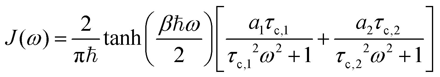 | (18) |
The dephasing rate, γm = 1/tD,m, and spectral density, Ji(ω), for every dye in each system provide a complete description of the system–bath component of the total Hamiltonian for that molecule (eqn (4)–(6)). We employ this description to realize the D–J algorithm with a realistic bath, by applying the same methodology used for the model bath in Section 4. Here, we solved the Redfield equations with J(ω) described by eqn (18), and using the parameters calculated in this section, i.e., tD, a1,2 and τc;1,2. The resulting time-dependent dynamics are shown in Fig. 7, for the constant combined and serial versions of the algorithm. For the serial case, we maximize fidelity by eliminating the trivial action of  (just the identity operator).
 | ||
| Fig. 7 Time-evolution of the populations in the constant version of the D–J algorithm with the calculated bath. (A) The population for the Cy3(C) dye as the wavefunction evolves through the first and last step. The transformation time, τ, for each step is marked with blue and red dotted lines, respectively. (B) The populations for all four dyes for the single-step in the combined approach. Here, a single τ is indicated with a black dotted line. The populations for the closed system corresponding to the exact Hamiltonian evolution are shown in dashed lines, in both serial and combined approaches. | ||
The fidelity of the cyanine-mapped algorithm is then calculated using eqn (8). We find the simulated geometries encode the constant D–J algorithm with final fidelities of (τcon) = 0.994 and (τ3) = 0.819, for the combined and serial circuits, respectively. We note these values are better than those obtained with a model bath, which is expected, as these fictitious systems loss their phase about 20 times faster than the realistically simulated circuits.
We note that in both simulated Hamiltonians,  and
and  , the oscillatory behaviour is non-periodic, which results in increased stability against environment fluctuations, at least within the timescale of interest. This suggests that circuit fidelity depends almost entirely on the choice of circuit geometry, and not on its coupling with the harmonic bath. More conclusive results require a more accurate treatment of the intermolecular coupling, as eqn (10) does not consider the effect of the thermal motion over the charge distribution of the individual dyes. While the limited study we present here cannot necessarily be generalized, we can safely state that design strategies that limit overall evaluate time and circuit-to-circuit exciton transfer will feature improved fidelity. To this end, the combined strategy is preferred, especially for simple computations with relatively few qubits.
6 Conclusions
In this manuscript, we have evaluated the possibility of mapping multi-step quantum operations into excitonic circuits by applying our methodology to the realization of the 2-qubit Deutsch–Jozsa algorithm. We show this implementation can be approached with two general strategies: one involving a mapping of the individual steps in the algorithm and the precise control of the initial state of each operation in the sequence (i.e., a serial approach), and a second one were the entire algorithm is mapped into a single excitonic circuit realizing the transformation (i.e., a combined approach).We have implemented these two strategies on a cyanine-based excitonic circuit, first by studying a model environment for the system–bath interaction, and second by explicitly simulating the thermal fluctuations with QM/MM simulations. In the first case, the artificial bath model revealed a significant fidelity decrease in the serial case. Although this result is not surprising, it is essential to understand the magnitude of improvement that can be achieved by a combined algorithm.
The explicitly simulated model reveled the same pattern. However, the complexity of some of the transformations, and the reduced conformational space employed to map those operations, resulted in low fidelities arising from the impossibility to map the quantum operation exactly into an excitonic circuit within the constrained search space. Surprisingly enough, however, these geometries resulted in non-periodic quantum dynamics, with an increased protection to the thermal environment. As a result, it was not possible to draw conclusive differences between the serial and combined approaches with the present simulation, since the fidelity is almost entirely dependent on our ability to find precise geometries. Future studies should look to expand the conformational search space, for example, by employing molecules with shorter band gaps. This improvement will be essential if we intend to map more complicated operations than those presented in this work. Future implementations must also consider that the accuracy of a given exciton construction will be determined on how close we can get to the spatial arrangement derived from the GA search, and small deviations from idealized molecular configurations can lead to significant changes in the expected Hamiltonian. Moreover, while the accuracy of the simulation used here is enough to gain a general understanding of the main features of the harmonic bath, more rigorous methods and extended sampling is required for a precise study of the open system performance of these circuits.
Finally, here we limit ourselves to describing the environmental effects in terms of the local bath, while the effect of intramolecular fluctuations and those characteristic of the macromolecule scaffolding (e.g., a DNA scaffold) were mostly ignored. As a result, the effect of the environment is possibly underestimated, and more detailed studies are needed to fully assess the fidelity of organic excitonic systems.
Conflicts of interest
There are no conflicts to declare.Acknowledgements
This work was supported by the U.S. Department of Energy (DOE), Office of Science, Basic Energy Sciences (BES) under Award DE-SC0019998. M. A. C thanks Ardavan Farahvash and Amro Dodin for helpful discussions. Part of the simulations in this manuscript was performed using resources of the National Energy Research Scientific Computing Center (NERSC), a U.S. Department of Energy Office of Science User Facility located at Lawrence Berkeley National Laboratory, operated under Contract No. DE-AC02-05CH11231.References
- M. A. Castellanos, A. Dodin and A. P. Willard, Phys. Chem. Chem. Phys., 2020, 22, 3048–3057 RSC.
- F. Fassioli, R. Dinshaw, P. C. Arpin and G. D. Scholes, J. R. Soc., Interface, 2014, 11, 20130901 CrossRef PubMed.
- R. Jimenez, S. N. Dikshit, S. E. Bradforth and G. R. Fleming, J. Phys. Chem., 1996, 100, 6825–6834 CrossRef CAS.
- G. R. Fleming, G. S. Schlau-Cohen, K. Amarnath and J. Zaks, Faraday Discuss., 2012, 155, 27–41 RSC.
- S. M. Hart, W. J. Chen, J. L. Banal, W. P. Bricker, A. Dodin, L. Markova, Y. Vyborna, A. P. Willard, R. Häner, M. Bathe and G. S. Schlau-Cohen, Chem, 2021, 7(3), 752–773 CAS.
- J. L. Banal, T. Kondo, R. Veneziano, M. Bathe and G. S. Schlau-Cohen, J. Phys. Chem. Lett., 2017, 8, 5827–5833 CrossRef CAS PubMed.
- L. Kringle, N. P. D. Sawaya, J. Widom, C. Adams, M. G. Raymer, A. Aspuru-Guzik and A. H. Marcus, J. Chem. Phys., 2018, 148, 085101 CrossRef PubMed.
- É. Boulais, N. P. D. Sawaya, R. Veneziano, A. Andreoni, J. L. Banal, T. Kondo, S. Mandal, S. Lin, G. S. Schlau-Cohen, N. W. Woodbury, H. Yan, A. Aspuru-Guzik and M. Bathe, Nat. Mater., 2017, 17, 159 CrossRef PubMed.
- C. P. Dietrich, M. Siegert, S. Betzold, J. Ohmer, U. Fischer and S. Höfling, Appl. Phys. Lett., 2017, 110, 043703 CrossRef.
- G. D. Scholes, G. R. Fleming, A. Olaya-Castro and R. van Grondelle, Nat. Chem., 2011, 3, 763–774 CrossRef CAS PubMed.
- E. A. Hemmig, C. Creatore, B. Wünsch, L. Hecker, P. Mair, M. A. Parker, S. Emmott, P. Tinnefeld, U. F. Keyser and A. W. Chin, Nano Lett., 2016, 16, 2369–2374 CrossRef CAS PubMed.
- D. Hayes, G. B. Griffin and G. S. Engel, Science, 2013, 340, 1431–1434 CrossRef CAS PubMed.
- E. Collini and G. D. Scholes, Science, 2009, 323, 369–373 CrossRef CAS PubMed.
- H.-J. Son, S. Jin, S. Patwardhan, S. J. Wezenberg, N. C. Jeong, M. So, C. E. Wilmer, A. A. Sarjeant, G. C. Schatz, R. Q. Snurr, O. K. Farha, G. P. Wiederrecht and J. T. Hupp, J. Am. Chem. Soc., 2013, 135, 862–869 CrossRef CAS PubMed.
- A. Montanaro, npj Quantum Inf., 2016, 2, 1–8 Search PubMed.
- D. Deutsch, A. Ekert, R. Jozsa, C. Macchiavello, S. Popescu and A. Sanpera, Phys. Rev. Lett., 1996, 77, 2818–2821 CrossRef CAS PubMed.
- L. K. Grover, Phys. Rev. Lett., 1997, 79, 325 CrossRef CAS.
- I. Buluta and F. Nori, Quantum Simulators, 2009, http://science.sciencemag.org/.
- M. Santha, Theory and Applications of Models of Computation, Springer Berlin Heidelberg, 2008, pp. 31–46 Search PubMed.
- M. A. Nielsen and I. L. Chuang, Quantum Computation and Quantum Information, 10th Anniversary Edition, Cambridge University Press, Cambridge; New York, 2011 Search PubMed.
- P. R. Kaye, R. Laflamme and M. Mosca, An introduction to Quantum Computing, Oxford University Press, New York, 1st edn, 2007 Search PubMed.
- D. Deutsch and R. Jozsa, Proc. R. Soc. London, Ser. A, 1992, 439, 553–558 CrossRef.
- R. Cleve, A. Ekert, C. Macchiavello and M. Mosca, Proc. R. Soc. London, Ser. A, 1998, 454, 339–354 CrossRef.
- I. L. Chuang, L. M. Vandersypen, X. Zhou, D. W. Leung and S. Lloyd, Nature, 1998, 393, 143–146 CrossRef CAS.
- S. Guide, M. Riebe, G. P. Lancaster, C. Becher, J. Eschner, H. Häffner, F. Schmidt-Kaler, I. L. Chuang and R. Blatt, Nature, 2003, 421, 48–50 CrossRef PubMed.
- L. Dicarlo, J. M. Chow, J. M. Gambetta, L. S. Bishop, B. R. Johnson, D. I. Schuster, J. Majer, A. Blais, L. Frunzio, S. M. Girvin and R. J. Schoelkopf, Nature, 2009, 460, 240–244 CrossRef CAS PubMed.
- K. Kuroda, T. Kuroda, K. Watanabe, T. Mano, K. Sakoda, G. Kido and N. Koguchi, Appl. Phys. Lett., 2007, 90, 51909 CrossRef.
- K. Feron, W. J. Belcher, C. J. Fell and P. C. Dastoor, Int. J. Mol. Sci., 2012, 13, 17019–17047 CrossRef CAS PubMed.
- I. Barth, J. Manz, Y. Shigeta and K. Yagi, J. Am. Chem. Soc., 2006, 128(21), 7043–7049 CrossRef CAS PubMed.
- W. T. Pollard and R. A. Friesner, J. Chem. Phys., 1994, 100, 5054–5065 CrossRef CAS.
- T. C. Berkelbach, T. E. Markland and D. R. Reichman, J. Chem. Phys., 2012, 136, 084104 CrossRef PubMed.
- H. P. Breuer and F. Petruccione, The Theory of Open Quantum Systems, Oxford University Press, 2007, vol. 1, pp. 1–656 Search PubMed.
- A. Ishizaki, T. R. Calhoun, G. S. Schlau-Cohen and G. R. Fleming, Phys. Chem. Chem. Phys., 2010, 12, 7319–7337 RSC.
- A. Montoya-Castillo, T. C. Berkelbach and D. R. Reichman, J. Chem. Phys., 2015, 143, 194108 CrossRef PubMed.
- M. Levitus and S. Ranjit, Q. Rev. Biophys., 2011, 44, 123–151 CrossRef CAS PubMed.
- S. M. Hart, J. L. Banal, M. Bathe and G. S. Schlau-Cohen, J. Phys. Chem. Lett., 2020, 11, 26 CrossRef PubMed.
- J. C. Chang, J. Chem. Phys., 1977, 67, 3901 CrossRef CAS.
- A. Farahvash, C. K. Lee, Q. Sun, L. Shi and A. P. Willard, J. Chem. Phys., 2020, 153, 074111 CrossRef CAS PubMed.
- C. I. Bayly, P. Cieplak, W. D. Cornell and P. A. Kollman, J. Phys. Chem., 1993, 97, 10269–10280 CrossRef CAS.
- C. Olbrich, J. Strümpfer, K. Schulten and U. Kleinekathöfer, J. Phys. Chem. Lett., 2011, 2, 1771–1776 CrossRef CAS PubMed.
- C. Olbrich and U. Kleinekathöfer, J. Phys. Chem. B, 2010, 114, 12427–12437 CrossRef CAS PubMed.
- A. Damjanović, I. Kosztin, U. Kleinekathö and K. Schulten, Phys. Rev. E: Stat., Nonlinear, Soft Matter Phys., 2002, 65, 031919 CrossRef PubMed.
- S. Valleau, A. Eisfeld and A. Aspuru-Guzik, J. Chem. Phys., 2012, 137, 224103 CrossRef PubMed.
- M. I. Mallus, M. Aghtar, S. Chandrasekaran, G. Lü, M. Elstner and U. Kleinekathö, J. Phys. Chem. Lett., 2016, 7, 1102–1108 CrossRef CAS PubMed.
- S. J. Jang and B. Mennucci, Rev. Mod. Phys., 2018, 90, 035003 CrossRef CAS.
- J. Wang, R. M. Wolf, J. W. Caldwell, P. A. Kollman and D. A. Case, J. Comput. Chem., 2004, 25, 1157–1174 CrossRef CAS PubMed.
- Y. Shao, Z. Gan, E. Epifanovsky, A. T. Gilbert, M. Wormit, J. Kussmann, A. W. Lange, A. Behn, J. Deng, X. Feng, D. Ghosh, M. Goldey, P. R. Horn, L. D. Jacobson, I. Kaliman, R. Z. Khaliullin, T. Kuś, A. Landau, J. Liu, E. I. Proynov, Y. M. Rhee, R. M. Richard, M. A. Rohrdanz, R. P. Steele, E. J. Sundstrom, H. L. Woodcock, P. M. Zimmerman, D. Zuev, B. Albrecht, E. Alguire, B. Austin, G. J. O. Beran, Y. A. Bernard, E. Berquist, K. Brandhorst, K. B. Bravaya, S. T. Brown, D. Casanova, C.-M. Chang, Y. Chen, S. H. Chien, K. D. Closser, D. L. Crittenden, M. Diedenhofen, R. A. DiStasio, H. Do, A. D. Dutoi, R. G. Edgar, S. Fatehi, L. Fusti-Molnar, A. Ghysels, A. Golubeva-Zadorozhnaya, J. Gomes, M. W. Hanson-Heine, P. H. Harbach, A. W. Hauser, E. G. Hohenstein, Z. C. Holden, T.-C. Jagau, H. Ji, B. Kaduk, K. Khistyaev, J. Kim, J. Kim, R. A. King, P. Klunzinger, D. Kosenkov, T. Kowalczyk, C. M. Krauter, K. U. Lao, A. D. Laurent, K. V. Lawler, S. V. Levchenko, C. Y. Lin, F. Liu, E. Livshits, R. C. Lochan, A. Luenser, P. Manohar, S. F. Manzer, S.-P. Mao, N. Mardirossian, A. V. Marenich, S. A. Maurer, N. J. Mayhall, E. Neuscamman, C. M. Oana, R. Olivares-Amaya, D. P. O'Neill, J. A. Parkhill, T. M. Perrine, R. Peverati, A. Prociuk, D. R. Rehn, E. Rosta, N. J. Russ, S. M. Sharada, S. Sharma, D. W. Small, A. Sodt, T. Stein, D. Stück, Y.-C. Su, A. J. Thom, T. Tsuchimochi, V. Vanovschi, L. Vogt, O. Vydrov, T. Wang, M. A. Watson, J. Wenzel, A. White, C. F. Williams, J. Yang, S. Yeganeh, S. R. Yost, Z.-Q. You, I. Y. Zhang, X. Zhang, Y. Zhao, B. R. Brooks, G. K. Chan, D. M. Chipman, C. J. Cramer, W. A. Goddard, M. S. Gordon, W. J. Hehre, A. Klamt, H. F. Schaefer, M. W. Schmidt, C. D. Sherrill, D. G. Truhlar, A. Warshel, X. Xu, A. Aspuru-Guzik, R. Baer, A. T. Bell, N. A. Besley, J.-D. Chai, A. Dreuw, B. D. Dunietz, T. R. Furlani, S. R. Gwaltney, C.-P. Hsu, Y. Jung, J. Kong, D. S. Lambrecht, W. Liang, C. Ochsenfeld, V. A. Rassolov, L. V. Slipchenko, J. E. Subotnik, T. Van Voorhis, J. M. Herbert, A. I. Krylov, P. M. Gill and M. Head-Gordon, Mol. Phys., 2015, 113, 184–215 CrossRef CAS.
- D. Case, I. Ben-Shalom, S. Brozell, D. Cerutti, T. Cheatham, III, V. Cruzeiro, T. Darden, R. Duke, D. Ghoreishi, M. Gilson, H. Gohlke, A. Goetz, D. Greene, R. Harris, N. Homeyer, Y. Huang, S. Izadi, A. Kovalenko, T. Kurtzman, T. Lee, S. LeGrand, P. Li, C. Lin, J. Liu, T. Luchko, R. Luo, D. Mermelstein, K. Merz, Y. Miao, G. Monard, C. Nguyen, H. Nguyen, I. Omelyan, A. Onufriev, F. Pan, R. Qi, D. Roe, A. Roitberg, C. Sagui, S. Schott-Verdugo, J. Shen, C. Simmerling, J. Smith, R. SalomonFerrer, J. Swails, R. Walker, J. Wang, H. Wei, R. Wolf, X. Wu, L. Xiao, D. York and P. Kollman, AMBER 2018, University of California, San Francisco, 2018 Search PubMed.
- Q. Sun, T. C. Berkelbach, N. S. Blunt, G. H. Booth, S. Guo, Z. Li, J. Liu, J. D. McClain, E. R. Sayfutyarova, S. Sharma, S. Wouters and G. K.-L. Chan, Wiley Interdiscip. Rev.: Comput. Mol. Sci., 2018, 8, e1340 Search PubMed.
- S. Mukamel, Principles of Nonlinear Optical Spectroscopy, Oxford University Press, New York, 1995, p. 543 Search PubMed.
Footnote |
| † Electronic supplementary information (ESI) available. See DOI: 10.1039/d1cp01643a |
| This journal is © the Owner Societies 2021 |