
 Open Access Article
 This Open Access Article is licensed under a Creative Commons Attribution-Non Commercial 3.0 Unported Licence
Glories, hidden rainbows and nearside–farside interference effects in the angular scattering of the state-to-state H + HD → H2 + D reaction
Chengkui
Xiahou
 a and
J. N. L.
Connor
*b
a and
J. N. L.
Connor
*b
aSchool of Pharmacy, Qilu Medical University, Zibo Economic Zone, Zibo City 255300, Shandong, People's Republic of China
bDepartment of Chemistry, The University of Manchester, Manchester M13 9PL, UK. E-mail: j.n.l.connor@manchester.ac.uk; Tel: +44-161-275-4693
First published on 18th May 2021
Abstract
Yuan et al. [Nat. Chem., 2018, 10, 653] have reported state-of-the-art measurements of differential cross sections (DCSs) for the H + HD → H2 + D reaction, measuring for the first time fast oscillations in the small-angle forward region of the DCSs. We theoretically analyse the angular scattering dynamics in order to quantitatively understand the physical content of structure in the DCSs. We study the H + HD(vi = 0, ji = 0, mi = 0) → H2(vf = 0, jf = 0,1,2,3, mf = 0) + D reaction for the whole range of scattering angles from θR = 0° to θR = 180°, where v, j, m are the vibrational, rotational and helicity quantum numbers respectively for the initial and final states. The restriction to mf = 0 arises because states with mf ≠ 0 have DCSs that are identically zero in the forward (θR = 0°) and backward (θR = 180°) directions. We use accurate quantum scattering matrix elements computed by Yuan et al. at a translational energy of 1.35 eV for the BKMP2 potential energy surface. The following theoretical techniques are employed to analyse the DCSs: (a) full and nearside–farside (NF) partial wave series (PWS) and local angular momentum theory, including resummations of the full PWS up to third order. We also use window representations of the scattering matrix, which give rise to truncated PWS, (b) six asymptotic (semiclassical) small-angle glory theories and four N rainbow theories, (c) we introduce “CoroGlo” tests, which let us distinguish between glory and corona scattering at small angles for Legendre PWS, (d) the semiclassical optical model (SOM) of Herschbach is employed to understand structure in the DCSs at intermediate and large angles. Our conclusions are: (a) the small-angle peaks in the DCSs arise mainly from glory scattering. For the 000 → 020 transition, there is also a contribution from a broad, or hidden, N rainbow, (b) at larger angles, the fast oscillations in the DCSs arise from NF interference, (c) the N scattering in the fast oscillation region contains a hidden rainbow for the 000, 020, 030 cases. For the 000 → 020 transition, the rainbow extends up to θR ≈ 60°; for the 000 and 030 cases, the angular ranges containing a N rainbow are smaller, (d) at intermediate and backward angles, the slowly varying DCSs, which merge into slow oscillations, are explained by the SOM. Physically it shows this structure in a DCS arises from direct scattering and is a distorted mirror image of the corresponding probability versus total angular momentum quantum number plot.
1. Introduction
The differential cross section (DCS) for a state-to-state transition in a chemical reaction is a very important observable in a molecular beam experiment, because it contains fundamental information on the dynamics and mechanism of the reaction.1–4 Recently (in 2018), Yuan et al.5 have reported the first experimental measurements of fast oscillations in the small-angle region for the degeneracy-averaged DCSs of a state-to-state reactive collision. They reported results for the following two transitions in the benchmark reaction (R1)| H + HD(vi = 0, ji = 0) → H2(vf = 0, jf = 1,3) + D | (R1) |
In addition, Yuan et al.5 reported an accurate quantum simulation of the experimental degeneracy-averaged DCSs. They observed very good agreement between the theoretical and measured results. The scattering computations of Yuan et al.5 were performed for the helicity-resolved state-to-state reaction
| H + HD(vi = 0, ji = 0, mi = 0) → H2(vf = 0, jf = 0,1,2,3, mf = 0,1,2,3) + D | (R2) |
 . Here J is the total angular momentum quantum number and θR is the reactive scattering angle, i.e., the angle between the incoming H atom and the outgoing H2 molecule in the centre-of-mass reference frame. Thus, θR = 0° and θR = 180° define the forward and backward directions respectively.
The purpose of this paper is to theoretically analyse the dynamics of the angular scattering for the H + HD reaction and to understand the physical content of structure in the DCSs. We consider the whole angular range, θR = 0°–180°, not just the small-angle region. Our analyses complement the computer simulation and results in ref. 5.
Before proceeding, we note there is a fundamental difference between the cases mf = 0 and mf ≠ 0 for reaction (R2). For mf ≠ 0, the scattering amplitudes, and hence the corresponding DCSs, are identically equal to zero at θR = 0° and θR = 180°. Only for mf = 0 are the DCSs non-zero in the forward and backward directions; this fact plays a key rôle in our analysis. This result is the consequence of conservation of angular momentum as embodied in the values of reduced rotation matrix elements at θR = 0° and θR = 180°. In this paper, we only consider the case mf = 0, with mf ≠ 0 analysed in a forthcoming paper. Thus the state-to-state reaction we consider is
| H + HD(vi = 0, ji = 0, mi = 0) → H2(vf = 0, jf = 0,1,2,3, mf = 0) + D | (R3) |
Our analysis will reveal the presence of the following physical phenomena in the DCSs as θR increases from 0°: forward glory scattering, which can merge into nearside–farside fast frequency oscillations, which can include a nearside broad or “hidden” rainbow, which can merge into direct scattering exhibiting slow frequency oscillations.
We employ the following theoretical tools in our analysis of structure in the DCSs:
• Partial wave theory
This includes the usual Legendre partial wave series for the scattering amplitude, together with a nearside–farside decomposition10–12 and local angular momentum theory,13–16 including resummations13–19 of the partial wave series up to third order. We also make use of truncated partial wave series arising from window representations20–22 of the scattering matrix.
• Forward glory scattering theory
To investigate the forward glory, we use the following asymptotic approximations from ref. 23–26: the integral transitional approximation, the semiclassical transitional approximation, the primitive and classical semiclassical approximations, and the uBessel approximation. We also use the 4Hankel approximation.27,28 Note that we use the words “asymptotic” and “semiclassical” interchangeably, with SC an abbreviation for semiclassical.
• Forward corona scattering theory
Yuan et al.5 drew attention to a qualitative analogy between the fast oscillations in the forward-angle region and the atmospheric corona phenomenon.29–33 We describe two tests, called “CoroGlo”, which let us distinguish, for a Legendre partial wave DCS, forward glory scattering from forward corona scattering.
• Nearside rainbow theory
We use the uniform and transitional Airy approximations;34 also the primitive and classical semiclassical approximations (which are different from the ones used for glory scattering).34
• Semiclassical optical model
This is a simple approximation for nearside direct scattering introduced by Herschbach.35,36 It is particularly useful for understanding structure at sideward and backward angles in the DCSs of direct reactions.
This paper is organised as follows. Section 2 outlines the partial wave theory that we use, and explains our conventions and definitions. The properties of the input scattering matrix elements are presented in Section 3. The results for the full, nearside and farside DCSs, including resummations, are described in Section 4. Next, in Section 5 we examine the properties of the quantum deflection function for the four transitions, as it is fundamental for the asymptotic (semiclassical) theories when they are applied to the scattering amplitudes. The six forward glory theories and their DCSs are described in Sections 6 and 7 respectively. In Section 8, we present the theory of corona scattering, together with the CoroGlo tests, which let us distinguish between glory and corona forward-angle scattering. The extraction of dynamical information from the fast oscillations at small angles in the DCSs is considered in Section 9. Our theories for a nearside rainbow and results are given in Sections 10 and 11 respectively. The theory of the semiclassical optical model is presented in Section 12, with the results for the angular scattering in Section 13. Our conclusions are in Section 14. The effect of resummation on a truncated partial wave series is discussed in the Appendix.
We do not report the results of every theoretical technique mentioned above, as applied to all four state-to-state transitions. Rather we often restrict our detailed discussion to just one transition, if a similar discussion also applies to the other transitions. Most of our results are presented graphically.
2. Partial wave representation
2.1 Partial wave series
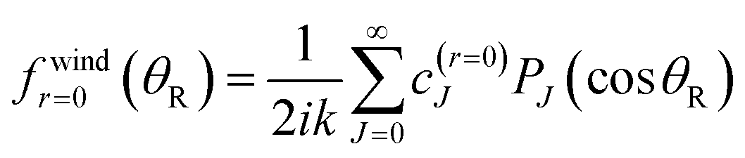
Since mi = mf = 0, the partial wave series (PWS) for the scattering amplitude can be expanded in a basis set of Legendre polynomials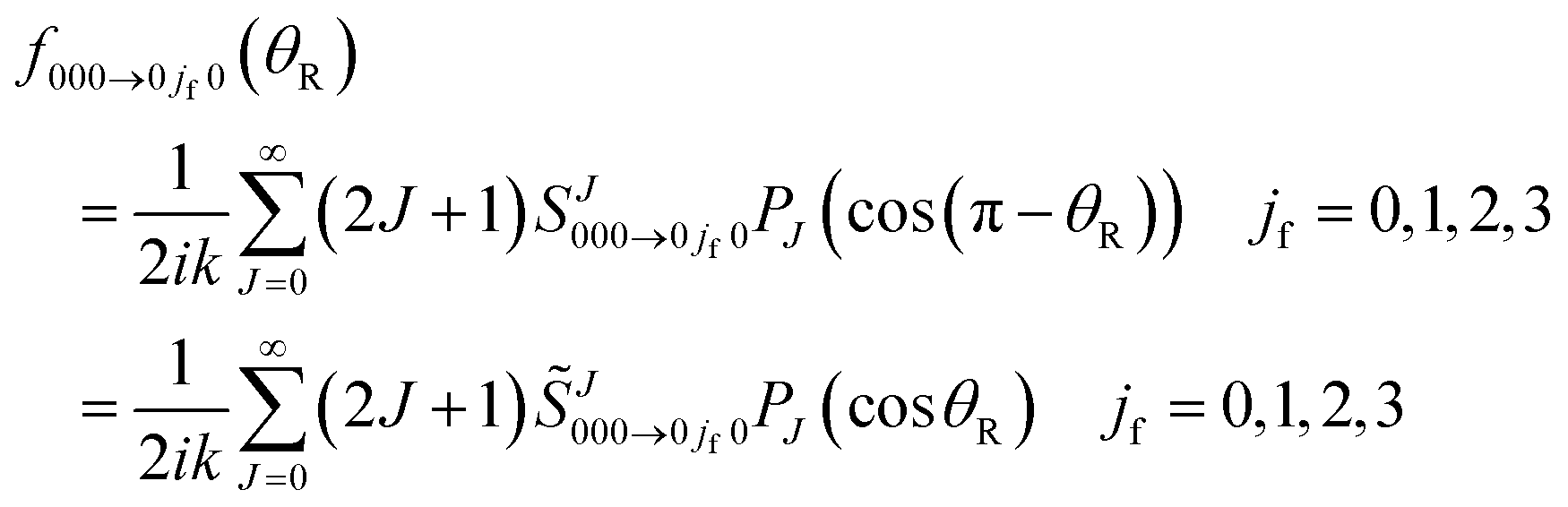 | (1) |
PJ(cos(π − θR)) = exp(iπJ)PJ(cos![[thin space (1/6-em)]](https://www.rsc.org/images/entities/char_2009.gif) θR) J = 0,1,2… θR) J = 0,1,2… |
where
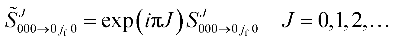
 is the Jth modified scattering matrix element. Also, k ≡ kvi=0,ji=0 is the initial translational wavenumber, J is the total angular momentum quantum number, PJ(•) is a Legendre polynomial of degree J, and θR is the reactive scattering angle. In practice, the upper limit of infinity in the PWS is replaced by a finite value, Jmax, assuming that all partial waves with J > Jmax are negligible.
The differential cross section (DCS) is then given by
| σ000→0jf0(θR) = |f000→0jf0(θR)|2 jf = 0,1,2,3 | (2) |
From now on, we will drop the subscript “000 → 0jf0” to keep the notation simple, and also write ![[S with combining tilde]](https://www.rsc.org/images/entities/i_char_0053_0303.gif) J in place of
J in place of  . In addition, when we continue the set {J} to real values of J, we will write, (J); this is required in the SC analyses. Other calculations on the H + HD reaction can be found in ref. 37–42.
We also report results for truncated partial wave series (tPWS), which arise when a window representation for the S matrix is input into eqn (1). We use as a window the subset, {J|J = 0 ≤ Ji < Jf ≤ J = Jmax}, and exclude the case where both Ji = 0 and Jf = Jmax. When using a tPWS it is necessary to interpret the resulting tDCS with caution, since partial waves with J < Ji and J > Jf have been neglected, as well as the interference between the partial waves in the window with the two omitted sets of partial waves.
Our results for the H + HD reaction show that the full DCSs calculated from eqn (1) and (2) often exhibit complicated oscillatory structures. To help understand these oscillations, we make a nearside–farside (NF) decomposition of the scattering amplitude. This is outlined next.
2.2 Nearside–farside decomposition
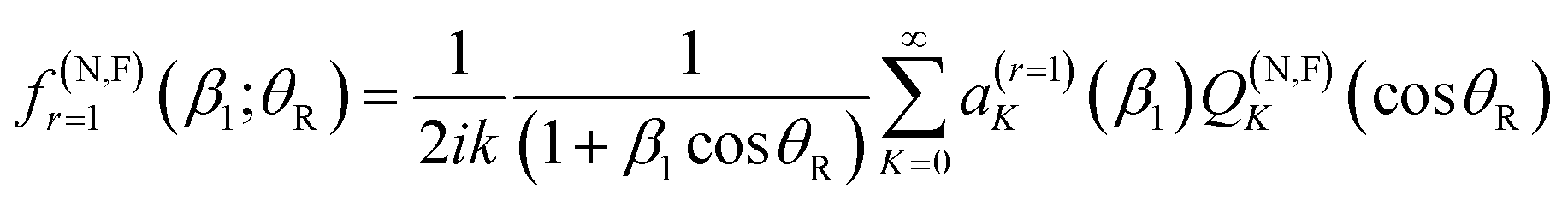
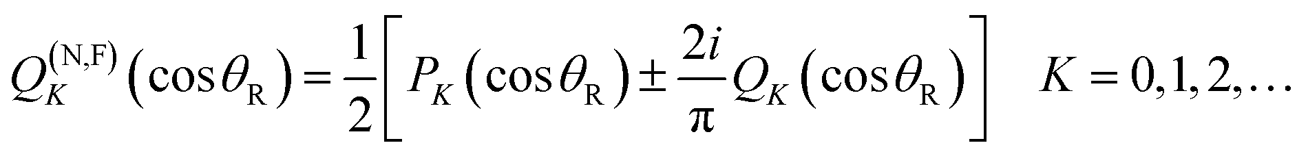
We exactly decompose the full scattering amplitude into the sum of two contributing terms, the N and F subamplitudes.10–12| f(θR) = f(N)(θR) + f(F)(θR) | (3) |
 | (4) |
 | (5) |
| σ(N,F)(θR) = |f(N,F)(θR)|2 | (6) |
which is the standard travelling angular wave interpretation.
A local angular momentum (LAM) analysis can also be used to provide information on the total angular momentum variable that contributes to the scattering at an angle θR, under semiclassical conditions.13–16 It is defined by
 | (7) |
 | (8) |
In eqn (4)–(6) and (8), we have used the Fuller NF decomposition,43 but there are available other NF decompositions for a Legendre PWS, namely those of Hatchell11,19,44 and Thylwe-McCabe.45 Note that NF DCS and NF LAM theories have been reviewed by Child (ref. 4, Section 11.2).
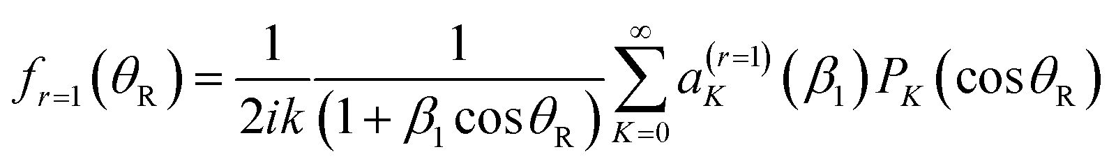
2.3 Resummation of the partial wave series
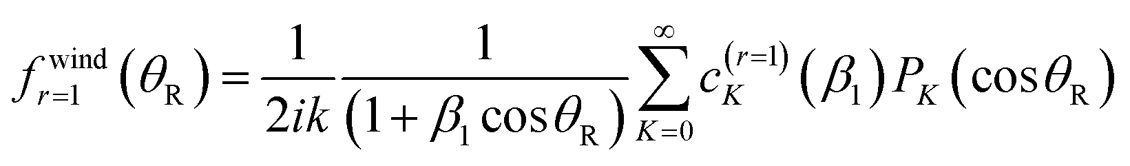
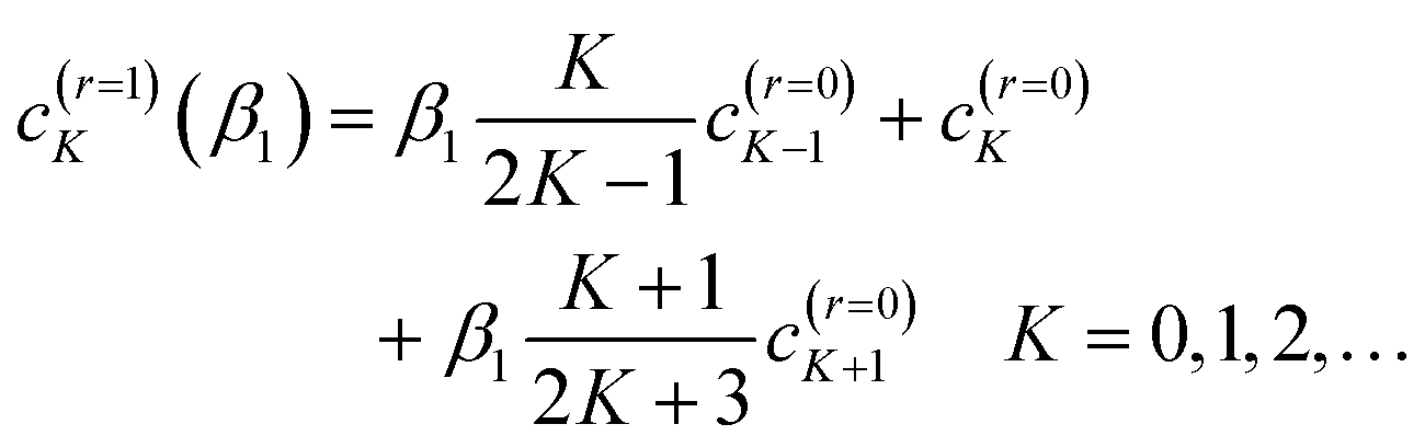
It is known that a resummation13–19 of the PWS (1) can significantly improve the physical effectiveness of the NF decomposition, (3)–(6). A detailed account of resummation theory for a Legendre PWS has been presented by Totenhofer et al.,19 so we do not repeat this material here.We have investigated resummation orders of r = 0 [no resummation, i.e., eqn (1)] and r = 1, 2, and 3. We find the biggest effect for cleaning the N,F DCSs and N,F LAMs of unphysical oscillations occurs on going from r = 0 to r = 1. Further resummations, r = 1 to r = 2, and, r = 2 to r = 3, have a smaller cleaning effect. Thus in the following we just summarise the r = 1 equations. Notice we sometimes label eqn (1) and related un-resummed equations with a subscript, r = 0.
Firstly we define
| aJ = (2J + 1)J J = 0,1,2,… | (9) |
 | (10) |
 | (11) |
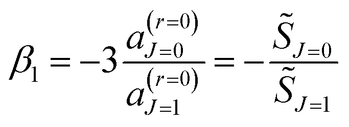
θR ≠ 0. We determine the real, or complex valued, resummation parameter, β1 ≡ β(r=1)1, in eqn (10) and (11) by solving a(r=1)J=0(β1) = 0, which yields β1 = −3a0/a1. This choice for β1 is the suggestion of Anni et al.13 A NF decomposition of eqn (10) can also be made. We write| f(θR) = f(N)r=1(β1;θR) + f(F)r=1(β1;θR) |
 | (12) |
with a0 =
 J=0.
J=0.
The corresponding N,F r = 1 resummed DCSs are then
| σ(N)r=1(β1;θR) = |f(N)r=1(β1;θR)|2 | (13) |
| σ(F)r=1(β1;θR) = |f(F)r=1(β1;θR)|2 | (14) |
 | (15) |
3. Properties of the input scattering matrix elements
The scattering calculations were performed5 for the Boothroyd–Keogh–Martin–Peterson potential energy surface number two (BKMP2).46 The numerical S matrix elements were computed by a time-dependent wave-packet method, which uses reactant Jacobi coordinates throughout the wave-packet propagation; also a second-order split operator procedure was employed to propagate the wave packet.5,38 Converged S matrix elements and DCSs were obtained for translational energies, Etrans, up to 3.5 eV.5In this paper, we consider S matrix elements at Etrans = 1.35 eV, for the transitions, 000 → 000, 000 → 010, 000 → 020, 000 → 030, which is the same translational energy as that employed in the experiments.5 We use masses of mH = 1.0078 u and mD = 2.0141 u; these correspond to an initial translational wavenumber of k = 11.692 a0−1. The values of Jmax are approximately 40 for each transition.
Fig. 1 shows graphs of |J| versus J for the four transitions, with the corresponding four graphs for argJ/rad versus J displayed in Fig. 2. On inspection of Fig. 1 and 2 we note the following:
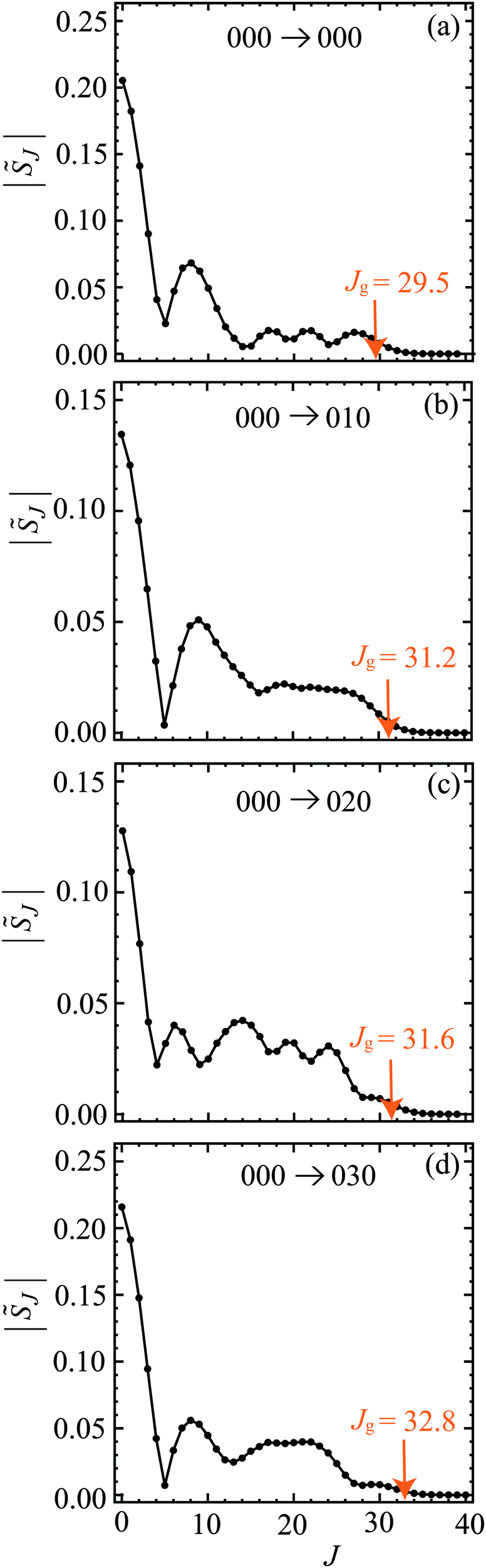 | ||
| Fig. 1 Plots of |J| versus J at Etrans = 1.35 eV. The black solid circles are the numerical S matrix data, {|J|}, at integer values of J, which have been joined by straight lines. An orange arrow indicates the value of the glory angular momentum variable, Jg. The transitions are: (a) 000 → 000, (b) 000 → 010, (c) 000 → 020, (d) 000 → 030. | ||
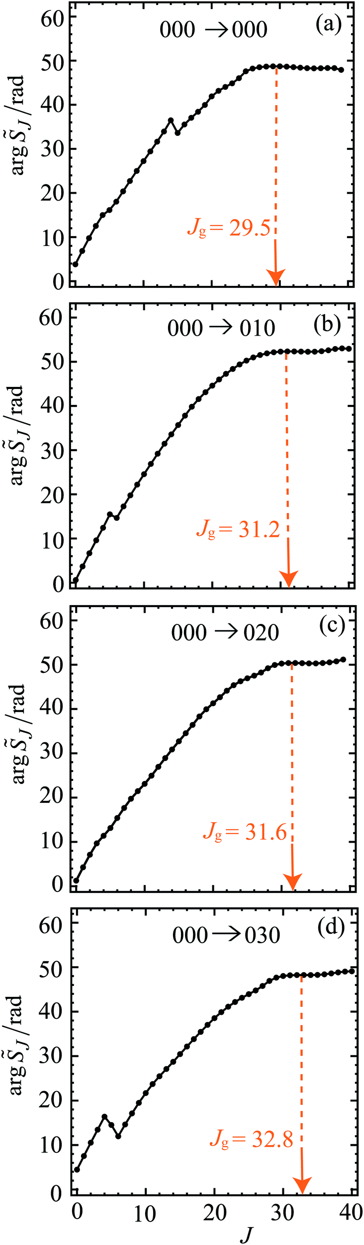 | ||
| Fig. 2 Plots of argJ/rad versus J at Etrans = 1.35 eV. The black solid circles are the numerical S matrix data, {argJ/rad}, at integer values of J, which have been joined by straight lines. An orange dashed line and orange arrow indicates the value of the glory angular momentum variable, Jg. The transitions are: (a) 000 → 000, (b) 000 → 010, (c) 000 → 020, (d) 000 → 030. | ||
• The maximum for a |J| plot occurs at J = 0 for all four transitions. As J increases, there are up to four noticeable subsidiary maxima. It can be seen that the first minimum occurs at J = 5, 5, 4, 5 for the 000, 010, 020, 030 cases respectively. The shapes of the |J| plots at low J play an important rôle in explaining structure in the DCSs at sideward and backward angles using the SOM theory, as will be demonstrated in Section 13. The relatively complicated shapes of the |J| plots are typical of other reactions involving H and D, for example, the H + D2 → HD + D reaction.23,24
• The plots of argJ/rad versus J are seen to be roughly quadratic in shape. The positions of the broad local maxima define the glory angular momentum variable, Jg, which has values in the range 29.5 to 32.8 for the four transitions. These values of Jg, are marked on Fig. 1 and 2, where it can be seen that |(Jg)|, and also (2Jg + 1)|(Jg)|, are not negligible. These results imply that Jg will be an important variable in the asymptotic (or SC) analysis of glory scattering in Sections 6 and 7. Also visible in Fig. 2 are kinks in the curves for the 000, 010, 030 cases. They occur when the corresponding |(J)| has a near-zero and the phase of (J) then varies more rapidly with respect to J.
4. Full and nearside–farside DCSs including resummations
Fig. 3 shows logarithmic plots of the full and N, F r = 1 DCSs versus θR for the four transitions. We use the following colour conventions for the DCSs, and in some other figures: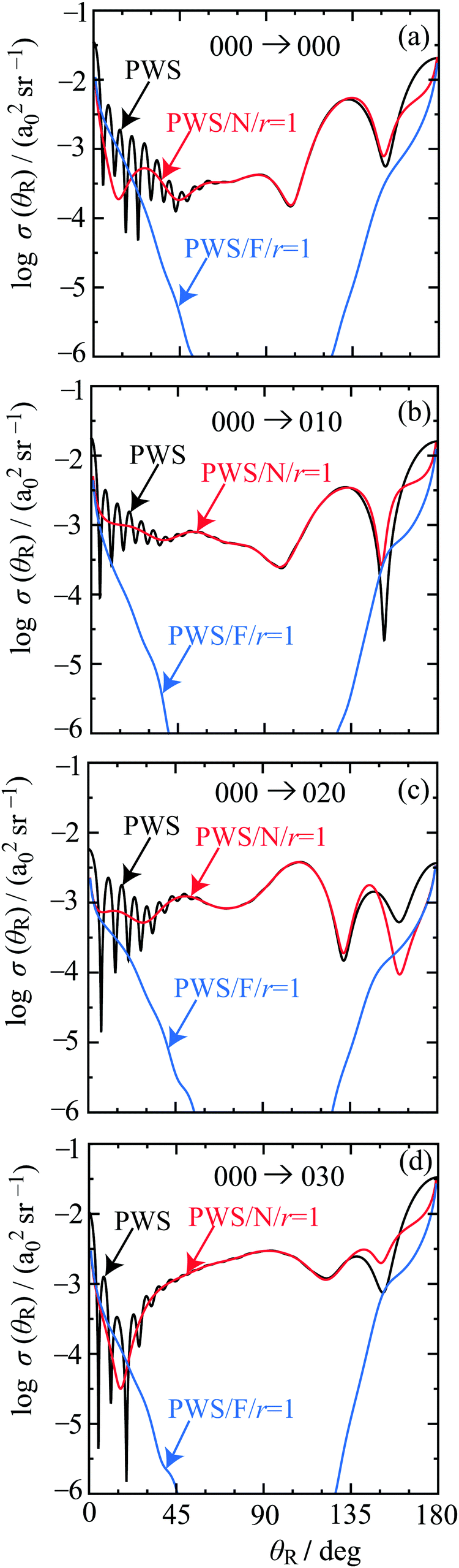 | ||
| Fig. 3 Plots of logσ(θR) versus θR at Etrans = 1.35 eV for: full PWS (black curve), N r = 1 PWS (red curve), F r = 1 PWS (blue curve). The transitions are: (a) 000 → 000, (b) 000 → 010, (c) 000 → 020, (d) 000 → 030. | ||
• Full PWS: black solid, with the label, PWS.
• N r = 1 PWS: red solid, with the label, PWS/N/r = 1.
• F r = 1 PWS: blue solid, with the label, PWS/F/r = 1.
The full DCS for the 000 → 000 transition is seen to exhibit the following properties as θR increases from 0° to 180°:
• A forward peak at θR = 0°, which merges into fast frequency oscillations, which damp out at θR ≈ 50°.
• An angular region extending from θR ≈ 50° to θR ≈ 100°, where the DCS varies more slowly.
• An angular region from θR ≈ 100° to θR = 180°, where there are pronounced slow frequency oscillations.
The DCSs for the other three transitions exhibit similar properties to the 000 case.
Next we examine the N, F r = 1 DCSs. Using the fundamental identity for N,F DCSs, e.g.ref. 19, we obtain important insights into structure occurring in the full DCSs. The fast frequency oscillations at forward angles, together with the forward peak are seen to arise from NF interference. Note that the variation of the N and F r = 1 DCSs with θR is slower than that for the corresponding full DCS. This behaviour is typical of glory scattering.24–26 It will be proven in Sections 6 and 7 using asymptotic techniques that the forward peak is indeed mainly a glory. The NF oscillations have a physical interpretation similar to the interference pattern from the well-known “Young's double slit” experiment – see Appendix A of ref. 47 for more details of this analogy in a scattering context. A useful result from this analogy is a simple approximate formula for the period of the oscillations, denoted ΔθR, namely
| ΔθR/rad ≈ π/Jeff | (16) |
In contrast, the scattering at sideward and backward angles is N dominated. Thus the NF analysis tells us the important result that the oscillations at forward and backward angles arise from different physical mechanisms. The results for the full and N, F r = 1 LAMs are consistent with those for the DCSs and are not shown.
To proceed further we need to undertake the much more difficult task of constructing the asymptotic (or SC) limit of the full and N, F PWS for each transition. This requires we first examine the properties of the quantum deflection functions, which are considered next.
5. Quantum deflection functions and their properties
The PW theory in Sections 2–4 uses the set of S matrix elements, {J}, with J = 0, 1, 2,…, Jmax. The asymptotic theory presented in Sections 6–13 requires the continuation of {J} to real values of J, which we denote by (J). That is, the S matrix elements are now considered to be a continuous function of the total angular momentum variable, J.
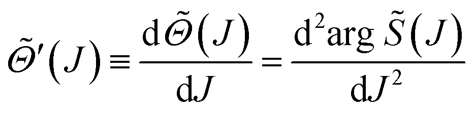
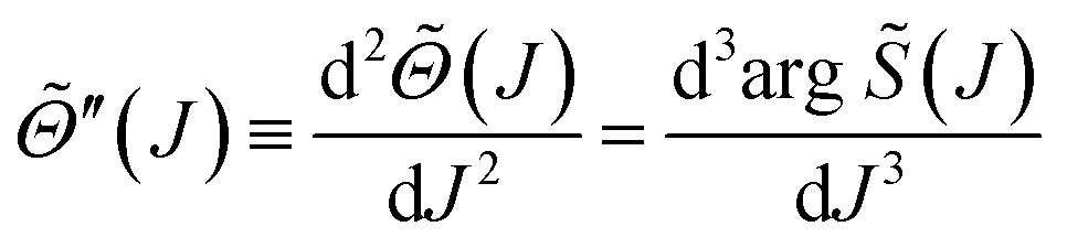
An important rôle in the SC analysis is played by the quantum deflection function (QDF), denoted ![[capital Theta, Greek, tilde]](https://www.rsc.org/images/entities/i_char_e134.gif) (J), and defined by
(J), and defined by
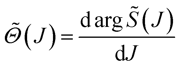 | (17) |
(J) curves).
Fig. 4 shows graphs of (J)/deg versus J for the four transitions. Cubic B-spline interpolation was usually used for the continuation of {J} to (J). Inspection of Fig. 4 reveals the following:
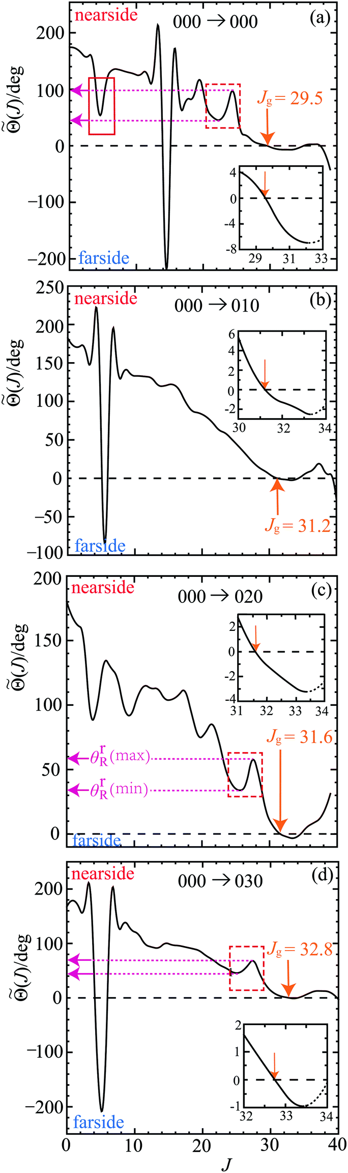 | ||
| Fig. 4 Plots of the QDF, (J)/deg, versus J, (black solid curve) at Etrans = 1.35 eV. An orange arrow indicates the value of the glory angular momentum variable, Jg, which satisfies (Jg) = 0. The inset shows the variation of (J)/deg close to J = Jg, where the black dotted curve indicates that the third branch of the QDF is not used in the SC glory analysis. The red solid rectangle encloses an example of a N rainbow (fold catastrophe) with a single minimum. The red dashed rectangles enclose two N rainbows with a minimum and a maximum, which together form part of a cusp catastrophe. The corresponding values of θrR(min) and θrR(max) are shown as pink dotted lines and pink arrows pointing toward the ordinate. The transitions are: (a) 000 → 000, (b) 000 → 010, (c) 000 → 020, (d) 000 → 030. | ||
• The curves for (J)/deg versus J are rather complicated with many maxima and minima.
• The most striking feature in the QDF plots are the steep dips, which occur for the 000, 010, 030 transitions. The minima of these dips occur for J ≈ 14.5, 5.5, 5.1 respectively and are evidently associated with the kinks in the argJ/rad plots of Fig. 2. Do we see noticeable structure in the DCSs associated with these dips? Inspection of Fig. 3 shows that the answer is no. We can understand this result because the contribution to a SC DCS, e.g. using the stationary phase approximation, is typically proportional to 1/|d(J)/dJ|. Now the moduli of the slopes are very large for a steep dip (except close to its minimum) and their contribution to the SC DCS will be very small. In addition, the two branches for each dip are separated by only a few J values, whereas a pronounced structure in a DCS, such as a rainbow, would typically involve a separation of many J values.
Contributions from these dips have been neglected in the following. We also note similar dips occur, and have been neglected, in the H + D2 → HD + D reaction – see in particular Fig. 2b of ref. 23 and Fig. 8 of ref. 24.
• Next we examine the QDF for the 000 → 000 transition in more detail:
– At small J there is N rainbow (minimum) of the Airy type (or fold catastrophe34). For clarity, it is enclosed in a red solid rectangle in Fig. 4(a).
– At larger J, marked by a red dashed rectangle, there is another N rainbow (minimum) of Airy type. It is close to a maximum in the QDF, so this whole structure is part of a cusp catastrophe.34
– At even larger J, we have a forward glory, where (Jg) = 0. The behaviour of (J) close to J = Jg is shown in the inset.
• We observe, similar to the 000 case, rainbows and glories in the QDF plots for the 010, 020, 030 transitions in Fig. 4(b)–(d).
6. Theory of forward glory scattering
In this Section, we give the working equations for six forward glory theories; the derivations can be found elsewhere.24–286.1 Preliminaries
We begin by defining our notation in Fig. 5(a), which shows a plot of(J)/deg versus J in the glory region, J = 28 to J = 33, for the 000 → 000 transition. On inspection of Fig. 5(a), we note the following:
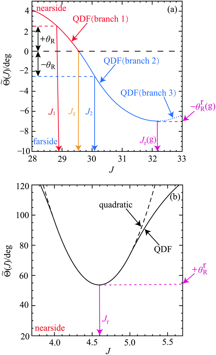 | ||
| Fig. 5 Plots for the 000 → 000 transition of Fig. 4(a) at Etrans = 1.35 eV giving the notations used in the SC glory and rainbow theories for all four transitions. (a) (J)/deg versus J close to J = Jg for the range J = 28 to J = 33. The three branches of the QDF used in the SC analysis are indicated: branch 1 (nearside, red solid curve), branch 2 (farside, blue solid curve) and branch 3 (farside, blue dotted curve). The values of (J)/deg at the angles +θR and −θR are indicated by a red dashed line (nearside) and a blue dashed line (farside) respectively. The corresponding values of the total angular momentum variable are denoted J1 ≡ J1(θR) (red solid arrow) and J2 ≡ J2(θR) (blue solid arrow) respectively. The orange arrow indicates Jg, which satisfies (Jg) = 0. The pink solid arrow shows the rainbow total angular momentum variable, Jr(g), which is close to Jg. The corresponding rainbow value of (J)/deg is denoted −θrR(g) (pink dashed line). (b) (J)/deg versus J for the range, J = 3.7 to J = 5.7. The pink solid arrow shows the rainbow total angular momentum variable, Jr. The corresponding nearside rainbow value of (J)/deg is denoted +θrR (pink dashed line). The black dashed curve shows the quadratic approximation to (J)/deg. | ||
• The real root of (J) = 0 occurs at J = Jg.
• The real root of the first derivative, d (J)/d J = 0, occurs at J = Jr(g), which defines the F rainbow angular momentum variable. The label “g” is added to indicate that Jr(g) is close to Jg, and to distinguish it from other N rainbows present in the full QDF plot, which are written, Jr – an example of a N rainbow is shown in Fig. 5(b). Note that (Jr(g)) = −θrR(g), with θrR(g) > 0 being the rainbow angle. It provides a natural boundary for the applicability of some of the glory theories described in Section 6.2. Inspection of Fig. 1 shows that |(J)| is very small for J > Jr(g), so contributions from this branch are neglected in our calculations.
• Semiclassically, J < Jg corresponds to N scattering; in contrast, J > Jg [with J ≤ Jr(g)] corresponds to F scattering.
• For (J) = +θR, where θR≥0, there is one real root, denoted J = J1 ≡ J1(θR), in the N scattering.
• For (J) = −θR, where 0 ≤ θR ≤ θrR(g) and J ≤ Jr(g), there is one real root, denoted J = J2 ≡ J2(θR), in the F scattering.
• For (J) = −θR, where θR > θrR(g), there are no real roots.
• For θR = 0, J1 and J2 coalesce to Jg.
• In the SC analysis, it is convenient to define three branches for the QDF in Fig. 5(a) as follows:
branch 1: 28 ≤ J < Jg (nearside)
branch 2: Jg < J < Jr(g) (farside)
branch 3: Jr(g) < J ≤ 33 (farside)
We also use the following notations, which follow from eqn (17):
 | (18) |
 | (19) |
 | (20) |
 | (21) |
 | (22) |
 | (23) |
All the glory theories described below are derived from the following Poisson integral24–27
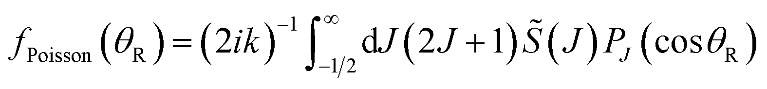 | (24) |
6.2 Six semiclassical forward glory DCSs
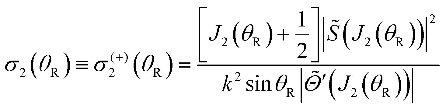
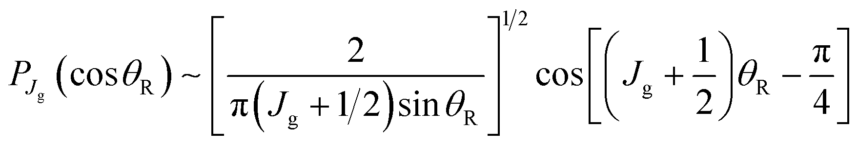
We next list the working equations for the DCSs of six SC forward glory scattering theories.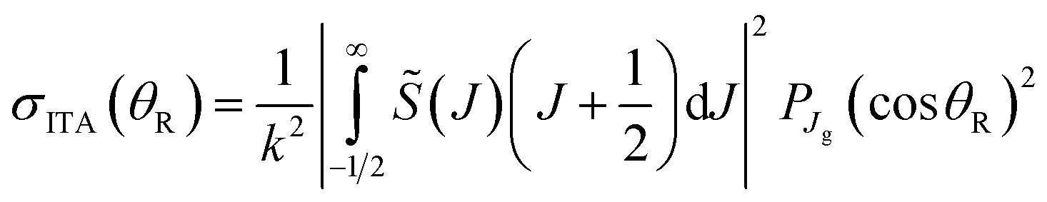 | (25) |
θR) is a Legendre function of the first kind. Also the ITA is exact for the Poisson integral (24) at θR = 0° because PJg(cos0) = 1.
In Section 8, we also need the ITA when the Hilb approximation is made for the Legendre function, namely24–26
 | (26) |
 | (27) |
 | (28) |
 | (29) |
 | (30) |
| σ4H(θR) = |f(−)4H(1|θR) + f(+)4H(2|θR)|2 | (31) |
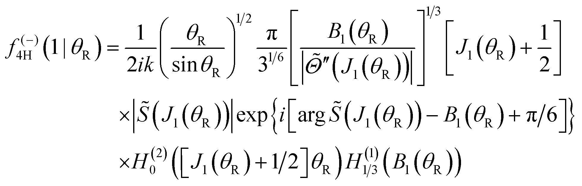 | (32) |
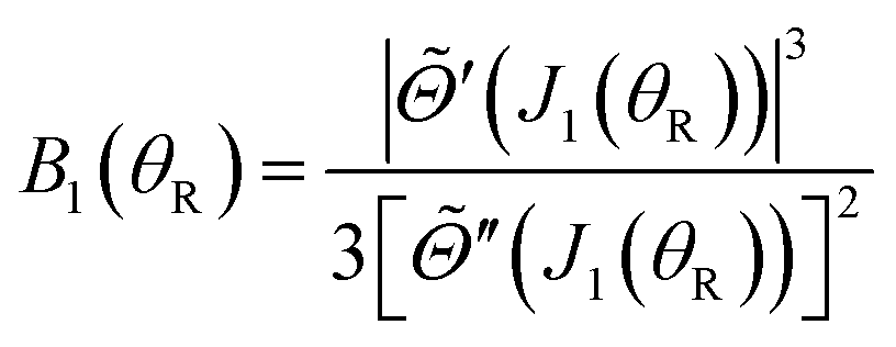 | (33) |
(J1) = +θR > 0.
On the farside, the second subamplitude is
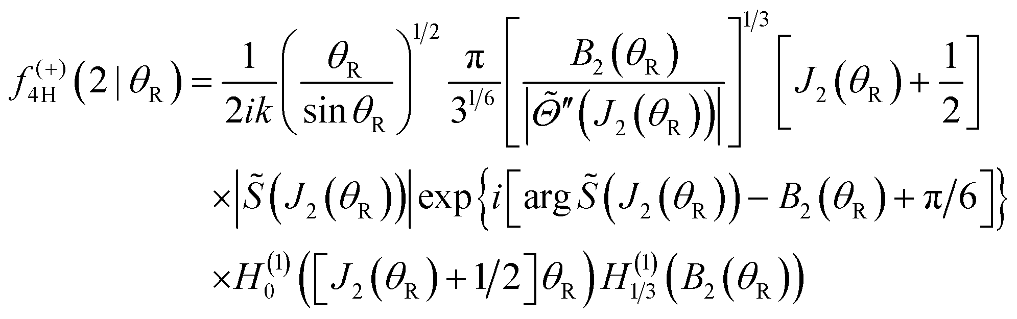 | (34) |
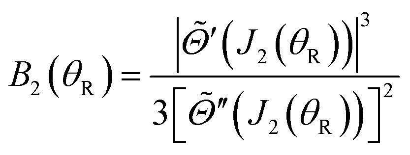 | (35) |
(J) = −θR is real. Thus in our calculations, we only apply the 4Hankel approximation (31) for 0 < θR < θrR(g). It diverges for θR → θrR(g).
 | (36) |
 | (37) |
Two special cases of the CSA are of interest – designated CSA/N and CSA/F – when we extract the N and F components from eqn (37) respectively. We have
| σCSA/N(θR) = σ1(θR) θR > 0 |
| σCSA/F(θR) = σ2(θR) 0 < θR < θrR(g) |
Some additional research on glories can be found in ref. 20–22 and 48–51.
7. Glory scattering results at forward angles
Fig. 6 and 7 show DCSs for the forward diffraction scattering in the range θR = 0°–10° for the four transitions. We are particularly concerned with the positions of the first minimum in the DCSs as they define the forward diffraction peaks. The following colour conventions are used for the DCSs in Fig. 6 and 7: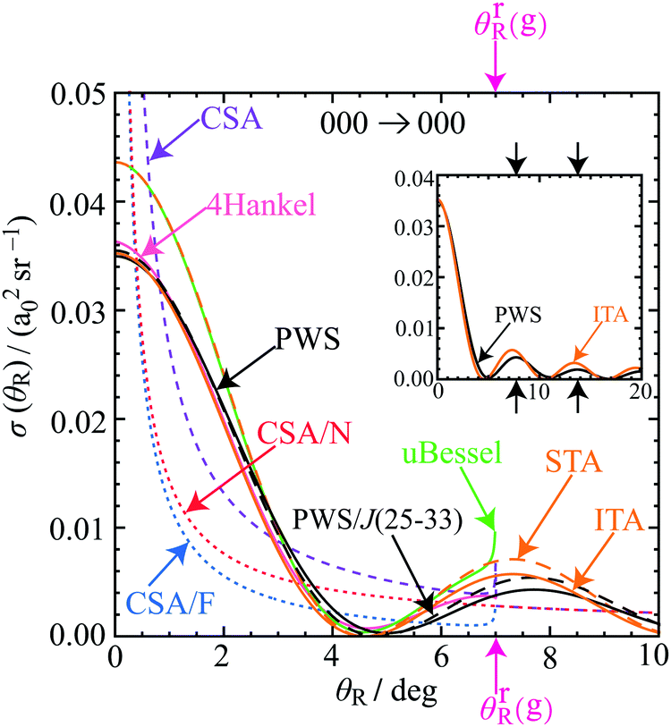 | ||
| Fig. 6 Plots of σ(θR) versus θR at Etrans = 1.35 eV for the 000 → 000 transition for the angular range θR = 0° to θR = 10°. The DCSs plotted are: PWS (black solid curve), PWS restricted to J = 25–33 (black dashed curve), ITA (orange solid curve), STA (orange dashed curve), uBessel (green solid curve), 4Hankel (pink solid curve). Also shown are the DCSs for CSA/F (blue dotted curve), CSA/N (red dotted curve) and their sum, CSA (lilac dashed curve). The pink rainbow angle in the glory region is denoted, θrR(g); it forms the natural boundary for the uBessel, 4Hankel, and CSA/F approximations. The inset shows the ITA DCS and PWS DCS for the angular range θR = 0° to θR = 20°, where the black arrows show the locations of two maxima, at θR = 7.71° and θR = 13.70°, for the PWS DCS. | ||
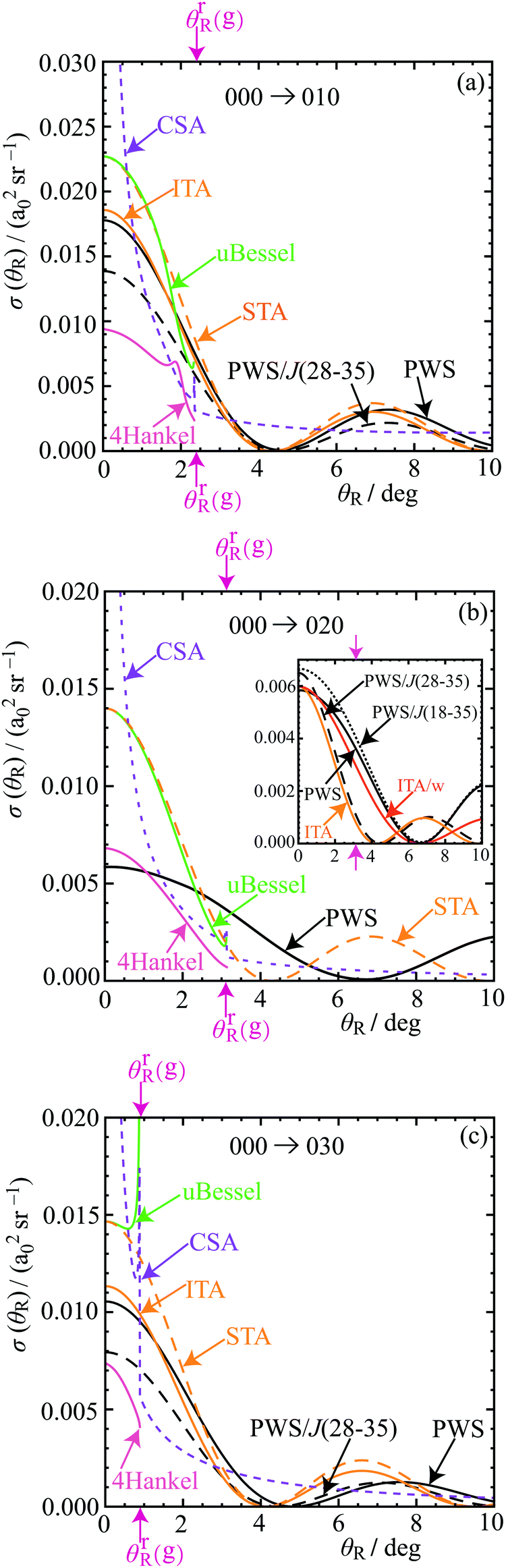 | ||
| Fig. 7 Plots of σ(θR) versus θR at Etrans = 1.35 eV for the (a) 000 → 010, (b) 000 → 020, (c) 000 → 030, transitions for the angular range, θR = 0° to θR = 10°. The DCSs plotted are: PWS (black solid curve), ITA (orange solid curve), STA (orange dashed curve), uBessel (green solid curve), 4Hankel (pink solid curve), CSA (lilac dashed curve). The pink rainbow angle in the glory region is denoted, θrR(g); it forms the natural boundary for the uBessel, 4Hankel, and CSA/F approximations, which forms part of CSA. Also shown are DCSs, (black dashed curves) for restricted PWS for J = 28–35. In the inset for (b) there are also plotted DCSs for PWS/J(18-35) (black dotted curve) and the weighted ITA, denoted ITA/w (orange solid curve). | ||
• Full PWS: black solid, with the label, PWS.
• tPWS: black dashed, with the label, PWS/J(25–33) for the window, J = 25(1)33. Likewise, PWS/J(28–35) and PWS/J(18–35).
• ITA and ITA/w: orange solid, with the label, ITA and ITA/w.
• STA: orange dashed, with the label, STA.
• 4Hankel: pink solid, with the label, 4Hankel.
• uBessel: green solid, with the label, uBessel.
• CSA: lilac dashed, with the label, CSA.
• CSA/N: red dotted, with the label, CSA/N.
• CSA/F: blue dotted, with the label, CSA/F.
We consider the 000 → 000 DCS in most detail, with less discussion for the 010, 030 cases, because they are similar to the 000 case. The 000 → 020 DCS exhibits some new features, which we analyse below.
7.1 DCSs for the 000 → 000 transition
The ITA and 4Hankel DCSs in Fig. 6 are seen to agree very well with the PWS DCS around its first minimum at θR ≈ 5.0°; this is also the case for the STA and uBessel DCSs, as well as for the PSA DCS (not shown). As we then decrease θR, we find the ITA and 4Hankel DCSs remain in close agreement with the PWS DCS, in particular at θR = 0°, although the STA and uBessel DCSs are somewhat larger. Notice the divergence of the 4Hankel, uBessel and CSA/F DCSs as θR → θrR(g) ≈ 7.0°. The CSA, CSA/N and CSA/F DCSs are useful because they show the trend in the scattering by passing through the oscillations. For θR > 10°, the ITA and STA DCSs drift out of phase relative to the PWS DCS, as expected. This is illustrated for the ITA DCS in the inset to Fig. 6 for θR ≤ 20°.We also show in Fig. 6 the DCS for a window tPWS, namely one with partial waves, J = 25(1)33. We observe good agreement with the full PWS DCS, which suggests this window includes the important dynamics responsible for the forward scattering. Indeed this is the case, since we use Jg = 29.5, in the SC glory theories.
7.2 DCSs for the 000 → 010 and 000 → 030 transitions
The PWS and SC glory DCSs for the 010 and 030 cases are displayed in Fig. 7(a) and (c) respectively. Also shown are the DCSs for a tPWS with a window of J = 28(1)35. The trends in the SC and tPWS DCSs are seen to be similar to the 000 case in Fig. 6, and will not be discussed further. Note that the F rainbow angles for these two transitions are θrR(g) ≈ 2.3° and θrR(g) ≈ 0.9° respectively, which are both close to θR = 0°. This means the range of applicability for the 4Hankel, uBessel and CSA/F approximations is very limited.7.3 DCSs for the 000 → 020 transition
The 000 → 020 DCSs in Fig. 7(b) and its inset exhibit more complicated behaviour. The F rainbow angle occurs at θrR(g) ≈ 3.1°, which again restricts the validity of the 4Hankel, uBessel and CSA/F approximations.Next, we observe that the first minimum in the PWS DCS curve occurs at θR ≈ 6.6°, whereas the corresponding minimum for the ITA DCS curve is at θR ≈ 4.3°. These minima are clearly visible in the inset to Fig. 7(b). To understand this difference, we note that a tPWS DCS using the window J = 28(1)35 agrees closely with the ITA DCS. This suggests there may be other dynamical effects for J ∉ {28,29,…,35} contributing to the PWS DCS [or equivalently to the Poisson DCS of eqn (24)].
The inset shows a second tPWS DCS, which uses a wider window, J = 18(1)35. We now observe much better agreement with the full PWS DCS, in particular around its minimum at θR ≈ 6.6°. Furthermore, inspection of the QDF in Fig. 4(c) shows there are two minima and two maxima (i.e., four Airy N rainbows), for the J-range starting at J = 18 and ending at J = 35. Semiclassically, this whole structure of four extrema corresponds to a swallowtail catastrophe.52 We expect there may be a contribution from the dark side of the deeper rainbow with a minimum near J ≈ 25.6. We will show that this is the case in Section 11, where we find there is a hidden rainbow present in the DCS for the angular range, θR ≈ 10°–60°.
The discussion just given implies there are one (or more) contributions to the Poisson integral (24) in addition to J values close to J = Jg. A straightforward way to improve the ITA is to multiply Jg by a weighting factor, w, to obtain an effective Jg-value, denoted Jwg, i.e., Jwg = wJg. We call this weighted approximation, ITA/w. With the choice, w = 0.64, we find, Jwg = 20.2. The inset shows the resulting ITA/w DCS, as well as the tPWS DCS with the window, J = 18(1)35, and we now observe much better agreement for these two DCSs with the full PWS DCS, especially around the minimum at θR ≈ 6.6°. Notice that Jwg = 20.2 is contained within the real interval, [18,35].
7.4 Conclusions
We have applied six SC glory theories, as well as tPWS, to the forward angle scattering for all four transitions. For the 000, 010, 030 cases, the ITA DCSs agree closely with the PWS DCSs, showing that the pronounced forward peak is indeed mainly a glory. The 000 case is the most favourable to analyse because it has the largest F rainbow angle of θrR(g) ≈ 7.0°. Smaller rainbow angles limit the applicability of the uBessel, 4Hankel and CSA/F approximations. The DCS for the 000 → 020 transition is more complicated. But our analysis showed that other dynamical effects are contributing to the scattering for the 020 case, in addition to the SC glory contribution.8. Theory of corona diffraction: tests for glory and corona small-angle scattering
Yuan et al. have suggested5 that the oscillatory small-angle scattering for the product DCSs of the H + HD reaction be called coronae, because of their qualitative resemblance to atmospheric coronae.29–33 Yuan et al. write “it is reasonable to make the analogy between the two phenomena” (ref. 5, Supplementary Information, p. 17). Here we quantitatively explore the similarities and differences between corona and glory small-angle scattering.An atmospheric corona is sometimes seen as a series of coloured concentric rings around the sun or moon, when they are partially covered by a thin mist or cloud.29–33 An atmospheric corona should not be confused with a solar (or stellar) corona, a coronavirus or a Corona beer.
Glories and coronae have some similarities in their small-angle scattering, as will be illustrated below. However, they are physically and mathematically distinct phenomena. We next present two small-angle ratio tests, which we collectively call “CoroGlo”. We then apply CoroGlo to the four PWS DCSs, thereby letting us distinguish between the presence of a glory or a corona in the forward scattering. The tests are adapted from results described by Canto and Hussein.53
8.1 CoroGlo test for a forward small-angle corona
A corona is usually modelled as Fraunhofer diffraction from a hard (impenetrable, rigid) sphere. In the SC limit, for a sphere of radius a, the DCS is given by29–33,53–59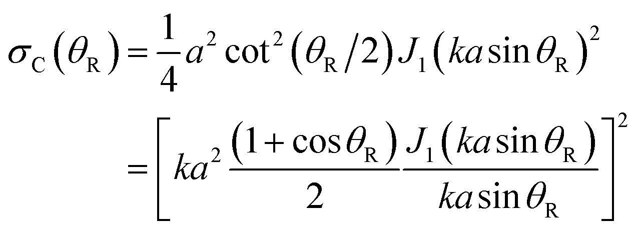 | (38) |
θR)/2 by 1 in eqn (38), yielding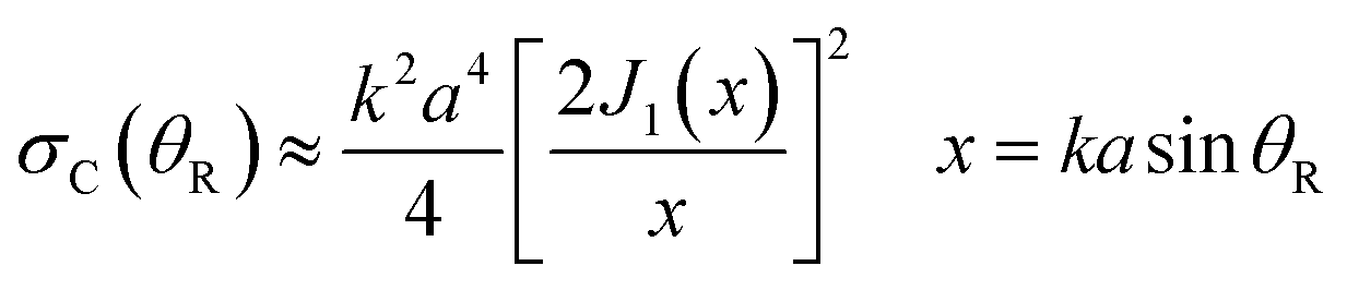 | (39) |
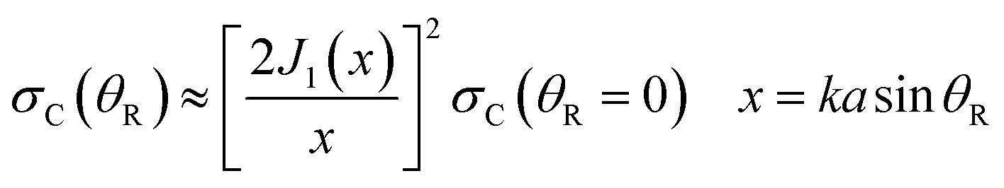 | (40) |
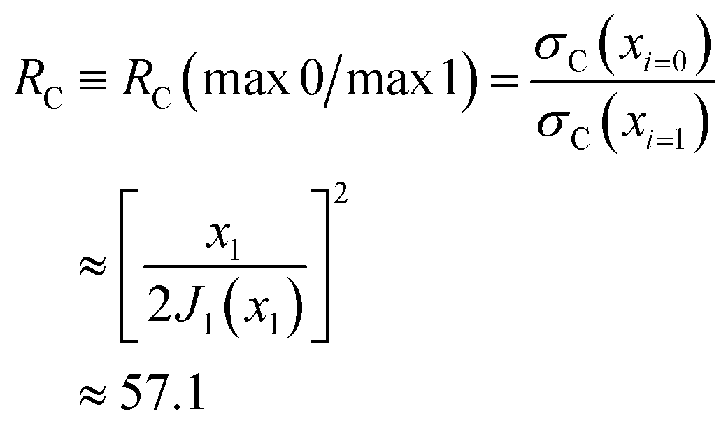
A corona can be characterized by the ratio of its primary maximum at x = 0 (or θR = 0) to the maxima of its subsidiary oscillations (ref. 53, p. 310) and in particular the adjacent maximum. We denote the locations of the maxima by xi with i = 0,1,2,… Thus, xi=0 = 0 and xi=1 = 5.14 – see Fig. 8. The corresponding values of the DCS are σC(x = xi=0 = 0) and σC(x = xi=1 = 5.14). Then the corona diffraction ratio (CDR) is defined as
 | (41) |
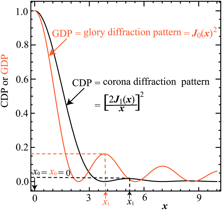 | ||
| Fig. 8 Plots of the CDP = corona diffraction pattern = [2J1(x)/x]2, (black solid curve) and the GDP = glory diffraction pattern = J0(x)2, (orange solid curve), versus x. The position of the principal maximum for both curves is at x0 = 0. The positions of the adjacent maxima for the CDP and GDP curves occur at x1 = 5.14 (black arrow) and 3.83 (orange arrow) respectively. | ||
In passing, we note that a straightforward method for finding the position, x1, of the i = 1 maximum in eqn (40) and (41) is to numerically solve d[2J1(x)/x]2/dx = 0. An alternative, simpler, method is to use the differential recurrence relation60
8.2 CoroGlo test for a forward small-angle glory
Next we derive a ratio test for a forward glory (ref. 53, p. 241) which we denote, RG ≡ RG(max0/max1), analogous to the corona ratio test, RC ≡ RC(max0/max1), of eqn (41). To do this, we employ the ITA/J0 approximation of eqn (25) and (26), in which the Legendre function is approximated by a Bessel function of order zero using the Hilb formula. In addition, since θR ≲ 10°, we can replace θR/sinθR by 1 to a very good approximation. We getSince, J0(0) = 1, we can also write
 | (42) |
The oscillations for both the CDP and the GDP arise from nearside–farside interference. This follows from the large x asymptotic approximation61
Similar to the corona case, we can characterize a glory by the ratio of its primary maximum at x = 0 (or θR = 0°) in the GDP to the maxima of its subsidiary oscillations, and in particular the adjacent maximum (ref. 53, p. 241). We denote the locations of the maxima of J0(x)2 by xj with j = 0,1,2,… Thus xj=0 = 0 and xj=1 = 3.83 – see Fig. 8. The corresponding values of the DCS are then σG(x = xj=0 = 0) and σG(x = xj=1 = 3.83). Next, we define the glory diffraction ratio (GDR) by
 | (43) |
8.3 Application of the CoroGlo corona and glory tests to PWS DCSs
In this section, we apply the CoroGlo corona and glory tests of eqn (41) and (43) respectively, to the PWS DCSs displayed in Fig. 3 for θR = 0°–180°, or in more detail in Fig. 6 and 7 for a smaller range of angles. We recall that the PWS DCSs have been calculated using accurate quantum S matrix elements and are in close agreement with the experimental results. We write RQ for the ratio of the forward diffraction peak to the adjacent maximum for the accurate quantum PWS DCSs. We obtain the following ratios:| 000 → 000: RQ = 8.1, |
| 000 → 010: RQ = 5.6, |
| 000 → 020: RQ = 2.6, |
| 000 → 030: RQ = 8.3. |
The RQ values for the 000, 010, and 030 cases are much closer to the GDR value of 6.2, which tells us that glory scattering makes a major contribution to the small-angle region for these cases. The results from this test are consistent with the SC glory analyses of Sections 6 and 7. Since the RQ values are not very close to 6.2, this implies (as expected) there are small contributions from other mechanisms.
The largest deviation from RG = 6.2 occurs for the 020 case, which suggests there is another, more significant, contribution to the small-angle scattering, in addition to the glory mechanism. This is consistent with the SC glory analysis of the PWS DCS in Fig. 7(b). In Sections 10 and 11, we will show that there is indeed a contribution from a hidden rainbow to the 020 PWS DCS.
9. Periods of the oscillations in the small-angle PWS DCSs
In Section 8.3, we showed that the height of the primary maximum in a DCS (located at θR = 0°) and the height of its adjacent maximum provided valuable information on the dynamics of the reaction via the CoroGlo tests. Now upon examination of Fig. 3, or in more detail in Fig. 6, 7 and 9, we see that the periods of the NF oscillations are approximately constant, usually in the range, 6°–7°. We next show how to obtain dynamical information from this observation.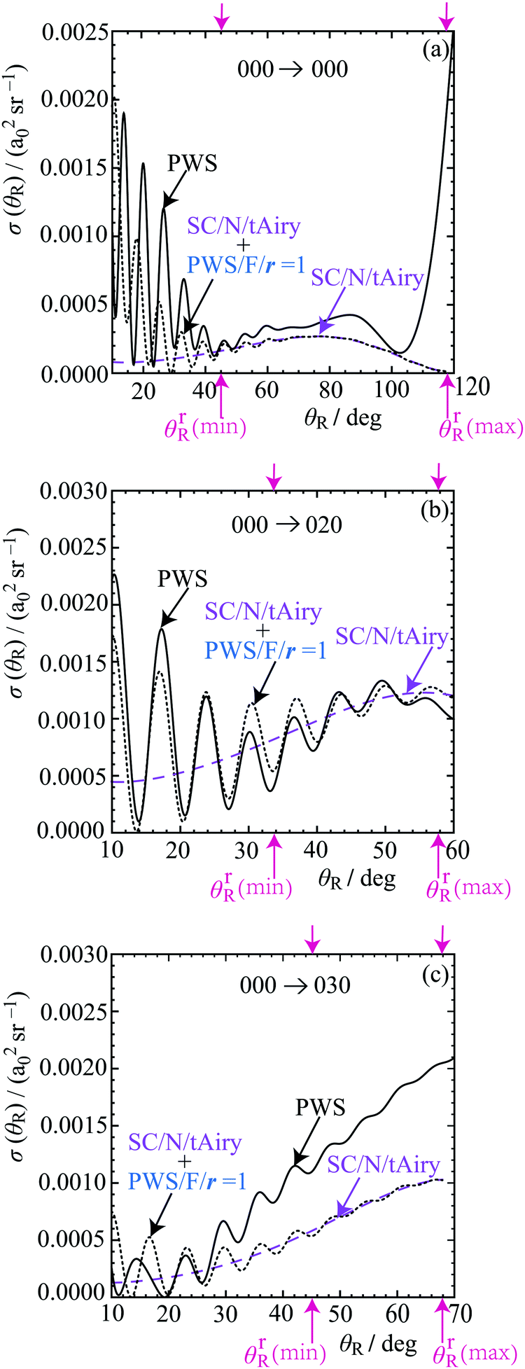 | ||
| Fig. 9 Plots of σ(θR) versus θR at Etrans = 1.35 eV. The DCSs plotted are: PWS (black solid curve), SC/N/tAiry (lilac dashed curve), SC/N/tAiry + PWS/F/r = 1 (black dotted curve). The pink arrows mark the locations of the rainbow angles, θrR(min) and θrR(max), which are also shown in Fig. 4. The transitions are: (a) 000 → 000 for θR = 10° to θR = 120°, (b) 000 → 020 for θR = 10° to θR = 60°, (c) 000 → 030 for θR = 10° to θR = 70°. | ||
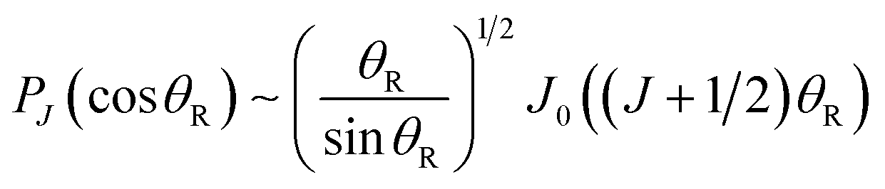
According to eqn (25), the dependence of the ITA DCS on θR is given by the square of the Legendre function, namely PJg(cosθR)2. This is also the case for the STA of eqn (27). Now for JgsinθR ≫ 1, we can use the asymptotic approximation62
 | (44) |
 | (45) |
We consider the 000 → 000 transition first. The inset to Fig. 6 shows that the ITA DCS closely follows the PWS DCS out to θR = 20°. The PWS DCS has maxima at θR = 7.71° and θR = 13.70°, so the period is, ΔθR/deg = 5.99. From eqn (45), we obtain Jg = 29.6, which is very close to the value Jg = 29.5 given by the maximum of the arg(J)/rad versus J graph in Fig. 2(a).
We next repeat the procedure just described for the 010, 020, 030 PWS DCSs. We obtain estimates for Jg of 28.6, 25.5, 26.0, which can be compared with the values 31.2, 31.6 (or 20.2 for ITA/w), 32.8 used in the ITA analysis respectively. The errors are now larger, being within 8–26% of the ITA values, which can be understood because the ITA DCSs become increasingly out-of-phase relative to the PWS DCSs, as θR increases beyond 10°. Nevertheless, these estimates are still useful given the simplicity of eqn (45).
10. Theory of nearside rainbow scattering
Inspection of the QDFs in Fig. 4 reveals the existence of many extrema, which correspond to Airy rainbows in the SC theory.52 The question then arises: are these rainbows also visible in the DCSs? Looking at Fig. 3, there are no obvious “pronounced” primary rainbows (plus supernumerary rainbows) of Airy type in the DCSs, similar to those found in elastic scattering.4,63 Note: it is now known that such pronounced primary rainbows plus their supernumeraries can indeed occur in the DCSs of state-to-state chemical reactions.64,65However there is another possibility. It has been proven using rigorous asymptotic techniques that “broad” F Airy rainbows can occur in state-to-state reactive DCSs. These broad rainbows have been found in the DCSs of the F + H2 → FH(vf = 3) + H reaction,27,66 both in simulations of the 1985 experiment of Neumark et al.,67 as well as in the more recent 2008 experiment of Wang et al.68 Broad Airy rainbows are also called “hidden”,64,65 because their appearance in a DCS is quite different from that of pronounced Airy rainbows. Indeed, it took 24 years66 before it was realized that the experimental DCSs of Neumark et al.67 contain a hidden rainbow. It is also important to stress that the hidden rainbows in the F + H2 reaction are F rainbows, whereas the rainbows in Fig. 4, which we discuss next, are N rainbows.
In the next two subsections, we have chosen four N rainbows in Fig. 4(a), (c) and (d) for further SC analysis for the 000, 020, 030 cases respectively, [two rainbows are in Fig. 4(a)]. The QDF curve for the 000 → 010 transition in Fig. 4(b) only possesses slight undulations with no prominent extrema, so we do not consider this case.
10.1 A single N rainbow in the QDF at small J
Inspection of Fig. 4(a) for the 000 → 000 transition shows there is a minimum in the QDF at small J, namely from J ≈ 3.7 to J ≈ 5.7. Including the dark (classically forbidden) side of the rainbow, the corresponding range for(J) is from ≈ 20° to ≈ 120°. This (J,(J)) rainbow region is enclosed by a red solid rectangle in Fig. 4(a) and is drawn in more detail in Fig. 5(b). We denote the rainbow angular momentum variable where d(J)/dJ = 0 by Jr and the corresponding rainbow angle by θrR, thus, (Jr) = +θrR.
There are two standard (although related) methods34 for calculating the SC N subamplitude for a QDF rainbow of the type shown in Fig. 5(b):
(a) The uniform semiclassical Airy approximation.34 In a systematic notation, this is denoted SC/N/uAiry, or uAiry for short. Now the uAiry approximation is straightforward to apply on the bright side of the rainbow, i.e., for θR > θrR, but not on its the dark side, i.e., for θR < θrR, because the roots of the stationary phase equation, (J) = +θR, are then complex valued – a situation which is awkward to handle for numerical input S matrix data.
If we replace the Airy functions in the uAiry approximation by their asymptotic forms, we obtain the primitive semiclassical approximation.34 We denote this by PSA/NN because it contains two N sub-subamplitudes and to avoid confusion with the PSA (≡ PSA/NF) that arises in the theory of glory scattering given in Section 6.2(e). Dropping the interference term in PSA/NN gives the classical semiclassical approximation, CSA/NN.
(b) The transitional semiclassical Airy approximation.34 In a systematic notation, this is denoted SC/N/tAiry, or tAiry for short. The tAiry makes a quadratic approximation for (J) about J = Jr, and Fig. 5(b) show this is accurate up to ≈ 90°. The tAiry approximation has the advantage that it can be applied on both the bright and dark sides of the rainbow, since it only depends on quantities defined at (Jr,θrR). Because we will be showing DCSs using the tAiry approximation in Section 11, we write down the N subamplitude here:
 | (46) |
 | (47) |
| σ(−)tAiry(θR) = |f(−)tAiry(θR)|2 | (48) |
Additional remarks:
(a) The N LAM for the tAiry approximation (46), denoted LAM(−)tAiry(θR), is approximately equal to −(Jr + 1/2), which is independent of θR.16,27
(b) The tAiry and uAiry approximations become equivalent for a quadratic QDF provided the pre-exponential factor is a constant in the original SC integral.34 For a numerical illustration, see example 1 in the Appendix of ref. 28.
(c) The tAiry approximation has also been applied in examples 2 and 3 of the Appendix of ref. 28 to two oscillating integrals of relevance to molecular scattering, namely a real-valued oddoid integral of order two and a complex-valued swallowtail integral.52 For both of these integrals, the tAiry approximation is in very good agreement with the exact numerical values in the dark regions.
(d) We can make a check on eqn (46) and (47) by putting |(Jr)| → 1 and arg(Jr) → 2δ(Jr); we then obtain a tAiry result that is equivalent to one arising in the SC theory of elastic cusped rainbows using the Pearcey integral [see eqn (3.40) and (3.41) of ref. 69].
10.2 Three N rainbows in the QDF at large J
Fig. 4 shows there are three N rainbows at large J which are indicated by red dashed rectangles. Their shapes on the inside-left of a rectangle are similar to the rainbow in Section 10.1 and Fig. 5(b), being approximately quadratic. The corresponding rainbow angle for this case is denoted, θrR(min). On the inside-right of the dashed rectangles, the QDFs bend over and there is a maximum. We denote the corresponding rainbow angle by θrR(max). The values of θrR(min) and θrR(max) are marked by pink arrows and dotted pink lines pointing towards the ordinates in Fig. 4.Having identified four N rainbows in the QDFs, we next carry out a SC analysis in the following section to see if these rainbows make an important contribution to the DCSs.
11. Nearside rainbow angular scattering results
We consider the four rainbows in the QDFs at small J and large J separately.11.1 Nearside rainbow scattering at small J
Firstly, we consider the N rainbow at small J in Fig. 4(a) for the 000 → 000 transition; it is enclosed by a red solid rectangle. Our main SC tool is the tAiry subamplitude of eqn (46) and (47). We find that the corresponding tAiry DCS of eqn (48) is very small. As a check, we have also applied the uAiry, PSA/NN, and CSA/NN approximations in the range, θR > θrR, and obtained the same result, i.e., there is no hidden rainbow present in the DCS. These findings also tell us that the widely-spaced oscillations for θR ≳ 90° in Fig. 3(a) are not a S matrix phase interference effect. Rather, in Section 13 we will use the SOM to show that these oscillations arise from the variation of |(J)| with J.
11.2 Nearside rainbow scattering at large J
Secondly, we consider the three N rainbows at large J in Fig. 4(a), (c) and (d) for the 000, 020, 030 cases respectively; they are enclosed by red dashed rectangles. Since we require results for θR < θrR(min), our main tool is again the tAiry approximation, although we have also used the uAiry, PSA/NN, and CSA/NN approximations for θR > θrR(min).Our results for the DCSs are plotted in Fig. 9. Notice that the abscissae start at θR = 10°, in order to overlap with Fig. 6 and 7, and end just beyond the θR = θrR(max) values. This is because the SC approximations we employ are not valid for θR ≳ θrR(max). Now the 000 → 020 transition has the smallest value of θrR(min) and no nearby additional rainbows, so we discuss the SC DCSs for this transition first.
Inspection of Fig. 9(b) shows that, σ(−)tAiry(θR), which is also labelled SC/N/tAiry and drawn as a lilac dashed curve, passes through the oscillations in the full PWS DCS. Next, we have added to the tAiry subamplitude, the contribution from the F r = 1 PWS subamplitude, which is also labelled PWS/F/r = 1. The resulting total DCS
| σ(F,r=1)tAiry(θR) = |f(−)tAiry(θR) + f(F)r=1(θR)|2 | (49) |
We can make another check on this rainbow. The PWS N LAM(θR) for r = 1, denoted LAM(N)r=1(θR), varies slowly in the range θR = 10°–60°, with a mean value of −26.2. For a N rainbow, we then expect the following relations to hold:16,27
| |〈LAM(N)r=1(θR)〉| ≈ |LAM(−)tAiry(θR)| ≈ Jr + 1/2 ≈ ReJ0 + 1/2 | (50) |
J}, in the range J = 10(1)33. Since, Jr = 25.4, we see that the approximations (50) are satisfied. This tells us that the PWS, SC and CAM theories are consistent in their descriptions of the angular scattering.
The rainbow scattering in Fig. 9(b) continues into the region, θR < 10°, thereby also making a contribution at small forward angles. In particular, it agrees well with the PWS DCS down to θR ≈ 2.5°. An additional mechanism was suggested by our SC glory analysis in Section 7.3, but not identified. Now we see a broad rainbow also contributes at small angles and is the unidentified mechanism.
Next we consider the DCSs for the 000 → 030 transition in Fig. 9(c). We see similar rainbow behaviour to the 020 case, but restricted to 20° ≲ θR ≲ 30°. We can understand this result from Fig. 4(d), which shows that the QDF minimum and maximum in the red dashed rectangle are rather close to each other, their angular separation being about 23°. This suggests a full SC analysis may require the uniform Pearcey asymptotic approximation;69 however this is beyond the scope of the present paper.
Finally, we examine the DCSs for the 000 → 000 transition in Fig. 9(a). This is similar to the 030 case in that the rainbow is confined to a small angular region, namely 30° ≲ θR ≲ 50°. Fig. 4(a) shows the presence of additional rainbows just outside the red dashed rectangle to its left, which will probably make an additional contribution to the tAiry subamplitude for θR ≳ 50°.
Some additional research on rainbows can be found in ref. 49, 53, 56–59 and 70–75.
11.3 Conclusions
This is the first report of N rainbows in the DCSs of state-to-state chemical reactions. The 020 case exhibited a broad or hidden rainbow over the angular range, 2.5° ≲ θR ≲ 60°. The 000 and 030 cases also showed hidden rainbow behaviour, but over a smaller range of angles.12. Semiclassical optical model (SOM): theory
The SOM is a simple procedure for calculating the DCSs of state-to-state chemical reactions. It was introduced by Herschbach35,36 and has subsequently been applied to several reactions.12,76–87 In addition, the SOM has been generalized to a “sticky optical model” for reactions which involve formation of a long-lived complex.47 In the NF terminology of Section 2, the SOM is an example of an (approximate) N theory. It is also a limiting case of the complex angular momentum (CAM) theory developed in ref. 47 for reactive angular scattering.Unlike the glory analysis of Section 6 – or the rainbow analysis of Section 10 – the SOM does not use the phase of each S matrix element, rather it employs just the moduli, |J|, or more precisely the corresponding reaction probability, defined by
| PJ ≡ |J |2 J = 0,1,2,… | (51) |
The SOM makes two assumptions:
Assumption 1. The reaction can be represented by the classical collision of two hard spheres. The classical DCS for a hard sphere collision is isotropic, being given by:
| σhs(θR) = (d/2)2 | (52) |
| b = dcos(θR/2) | (53) |
For hard-sphere scattering, do not confuse the classical DCS of eqn (52) with the quantum diffraction DCS of eqn (38), as used in the theory of coronae.
Assumption 2. The role of the transferred atom is to determine which impact parameters lead to reaction. If we denote the reaction probability distribution function by P(b), then the DCS for the SOM is obtained by multiplying σhs(θR) by the reaction probability distribution function:
| σSOM(θR) = (d/2)2P(b(θR)) | (54) |
To obtain P(b), we assume that b ≈ J/k. For the four state-to-state reactions that we analyse in Section 13, we always have ji = 0, thereby justifying this approximation, which neglects the difference between total and orbital angular momentum. We can now write, P(b) ≈ PJ ≡ P(J), so that
| σSOM(θR) = (d/2)2P(J(θR)) | (55) |
| J(θR) = kdcos(θR/2) | (56) |
The two assumptions of the SOM imply that, in practice, it should work best for rebound collisions. These result from a repulsive interaction between the reacting partners, which gives rise to predominantly backward scattering. Notice that d is the only adjustable parameter in the SOM model.
13. SOM results:DCSs at intermediate and backward angles
The DCSs calculated using the SOM are shown in Fig. 10 for the four transitions. The abscissae on the graphs go from θR = 50° to θR = 180°, thereby providing overlap with Fig. 9. For each transition, two SOM DCS curves are shown. | ||
| Fig. 10 Plots of σ(θR) versus θR at Etrans = 1.35 eV for the angular range, θR = 50° to θR = 180°. The DCSs plotted are: PWS (black solid curve), SOM (red solid curve), SOM/scaled at θR = 180°(red dashed curve). The transitions are: (a) 000 → 000 using d = 1.71 a0, (b) 000 → 010 using d = 1.80 a0, (c) 000 → 020 using d = 1.90 a0, (d) 000 → 030 using d = 1.80 a0. | ||
For the first curve, d is chosen to fit approximately the first minimum in the slow frequency oscillations of the PWS DCS, as θR moves down from θR = 180°. This first SOM DCS is drawn as a red solid curve. The fit used the Manipulate[•] command in Mathematica 12.1.1. For the second curve, the previous SOM DCS has been scaled to the value of the PWS DCS at θR = 180°. We call this second fit, SOM(scaled), and the corresponding DCS is drawn as a red dashed curve in Fig. 10.
Next we compare the SOM DCSs with the PWS DCSs. We observe satisfactory agreement with the PWS DCSs for θR ≳ 50°, which includes the flattish PWS DCS at intermediate scattering angles. These results are encouraging considering the simplicity of the SOM, with eqn (55) and (56) telling us that the SOM and PWS DCSs are distorted mirror images of the corresponding PJversus J plots.
In more detail, we see the SOM(scaled) DCS agrees closely with the backward peak in the PWS DCS for all four transitions, whilst the SOM shows reasonable agreement with the first minimum and the first maximum, as we move to smaller angles away from the backward direction. As expected, the SOM nor SOM(scaled) does not reproduce the oscillatory PWS DCSs for θR ≲ 50°(not shown).
The values of d for the 000, 010, 020, 030 cases are similar, being d/a0 = 1.71,1.80,1.90,1.80, respectively. Note that the corresponding values of kd, which are used in eqn (56), are 20.0, 21.0, 22.2, 21.0. We can also compare the values of d with the saddle point properties of the BKMP2 potential energy surface. Now BKMP2 has a collinear symmetric saddle point with r‡HH = 1.757 a0 and r‡HD = 1.757 a0, so that d‡ = r‡HH + r‡HD = 3.514 a0.46 We observe that all four d values satisfy d < d‡. This result is consistent with the backward scattering arising from small impact parameters – or equivalently small values of J – rather than being determined by the saddle point geometry.
14. Conclusions
We have investigated quantitatively the angular scattering dynamics of the state-to-state reaction, H + HD(vi = 0, ji = 0, mi = 0) → H2(vf = 0, jf = 0,1,2,3, mf = 0) + D for the whole range of angles from θR = 0° to θR = 180°. The restriction to mf = 0 arose because states with mf ≠ 0 have DCSs that are identically zero in the forward (θR = 0°) and backward (θR = 180°) directions. The input to our analyses consisted of accurate quantum scattering matrix elements computed by Yuan et al. for the BKMP2 potential energy surface at a translational energy of 1.35 eV. The theoretical techniques used were: full and N, F PWS and LAMs, including resummations of the full PWS, up to r = 3. We also used tPWS arising from window representations of the scattering matrix.To investigate the asymptotic limits of the Legendre PWS, we employed six SC small-angle glory theories and four N rainbow theories. We introduced CoroGlo tests in order to distinguish between corona and glory scattering at small angles. Finally, we used the SOM theory of Herschbach to understand structure in the DCSs at intermediate and large angles.
We reached the following conclusions:
• The small-angle peaks in the DCSs come mainly from forward glory scattering. For the 020 case, there is also a contribution from a broad N rainbow.
• At larger angles, the fast oscillations in the DCSs arise from NF interference. The N scattering contains a broad, or hidden, rainbow for the 000, 020, 030 cases. For the 000 → 020 transition, the rainbow extends up to θR ≈ 60°; for the 000 and 030 cases, the angular ranges exhibiting a N rainbow are smaller.
• The periods of the fast NF oscillations can be used to estimate Jg.
• At intermediate and backward angles, the slowly varying DCSs, which merge into slow oscillations, are explained by the SOM. Physically it shows that structure in a DCS is a distorted mirror image of the corresponding PJversus J plot.
Conflicts of interest
There are no conflicts to declare.Appendix
In this appendix, we discuss how a resummation affects the N and F scattering subamplitudes for a window representation of the S matrix, which in turn gives rise to a truncated PWS. To make this Appendix self-contained, we first recall the following results for the resummation of the full scattering amplitude, where we write r = 0 for the un-resummed amplitude. We have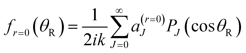 | (A1) |
| a(r=0)J = (2J + 1)J J = 0,1,2,… | (A2) |
It is known that a single resummation, r = 1, applied to eqn (A1) and (A2) gives13–19
 | (A3) |
θR ≠ 0, where β1 ≡ β(r=1)1 is the real-, or complex-, valued resummation parameter, and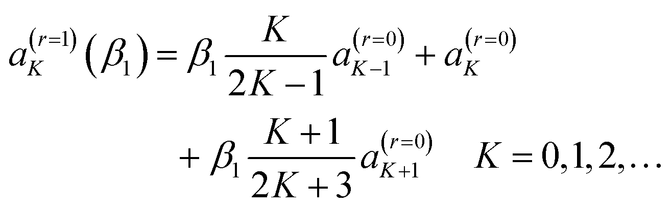 | (A4) |
cosθR)−1 has been removed from the PWS.13
The N, F r = 1 resummed subamplitudes are given by (with θR ≠ 0,π for the Fuller decomposition):13–19
 | (A5) |
An alternative form of eqn (A5) is the identity13,19
 | (A6) |
 | (A7) |
Definition. A window representation of the S matrix employs a finite proper subset of non-zero elements taken from the set {J|J = 0,1,2,…,J = Jmax}. In our applications, we use as a window the subset {J|J = 0 ≤ Ji < Jf ≤ J = Jmax}, and exclude the case where both Ji = 0 and Jf = Jmax. Typically, the values of J from J = Ji to J = Jf are chosen so that the corresponding {J} reproduce some important aspect(s) of the angular scattering.
Remark. When we have a full PWS with Ji = 0 and Jf = Jmax, the term “window representation” is also used in the literature in a different, although related, context.19,88,89 It is used when an exact rearrangement of the full PWS results in the main numerical contribution coming from a subset of S matrix elements – also called the window region.19,88,89
Using the definition above, we can now write the window scattering amplitude for r = 0 as
 | (A8) |
 | (A9) |
 | (A10) |
 | (A11) |
 | (A12) |
We next apply the identity (A6) to eqn (A11), which gives for the N, F r = 1 subamplitudes
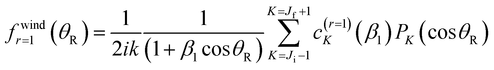
Now from eqn (A9) with Ji ≥ 1, we see that c(r=0)J=0 = 0. So the above equation simplifies to
| fwind,(N,F)r=1(β1;θR) = fwind,(N,F)r=0(θR) | (A13) |
When performing computations, we need a value for β1. By analogy with the Anni et al. prescription,13 we determine β1 when Ji ≥ 1 by solving  , which leads to
 | (A14) |
Finally we note that the results presented above can be generalized to resummation orders, r = 2, 3, 4,… with resummation parameters {β(r=2)1, β(r=2)2}, {β(r=3)1, β(r=3)2, β(r=3)3}, {β(r=4)1, β(r=4)2, β(r=4)3, β(r=4)4}…, provided that Ji ≥ 2, Ji ≥ 3, Ji ≥ 4,… respectively.
Acknowledgements
We thank Professor Zhigang Sun (State Key Laboratory of Molecular Reaction Dynamics, Dalian Institute of Chemical Physics, Chinese Academy of Sciences, Dalian 116023, Liaoning, People's Republic of China) for his help and for supplying scattering matrix elements. Support of this research is gratefully acknowledged by the P.R. China Project of Shandong Province Higher Educational and Technology Program, 2017, project number: J17KB068, and the Zibo School and City Integration Platform Project – Applied Pharmaceutical Innovation Platform (project number: 2018ZBC423).References
- W. Hu and G. C. Schatz, J. Chem. Phys., 2006, 125, 132301 CrossRef PubMed.
- A. Laganà and G. A. Parker, Chemical Reactions: Basic Theory and Computing, Springer International Publishing, Cham, Switzerland, 2018 Search PubMed.
- N. E. Henriksen and F. Y. Hansen, The Microscopic Foundation of Chemical Kinetics, Oxford University Press, Oxford, UK, 2nd edn, 2019 Search PubMed.
- M. S. Child, Semiclassical Mechanics with Molecular Applications, Oxford University Press, Oxford, UK, 2nd edn, 2014 Search PubMed.
- D. Yuan, S. Yu, W. Chen, J. Sang, C. Luo, T. Wang, X. Xu, P. Casavecchia, X. Wang, Z. Sun, D. H. Zhang and X. Yang, Nat. Chem., 2018, 10, 653 CrossRef CAS PubMed.
- J. Sang, D. Yuan, W. Chen, S. Yu, C. Luo, S. Wang, T. Wang, X. Yang and X. Wang, Chin. J. Chem. Phys., 2019, 32, 123 CrossRef CAS.
- D. Yuan, Y. Guan, W. Chen, H. Zhao, S. Yu, C. Luo, Y. Tan, T. Xie, X. Wang, Z. Sun, D. H. Zhang and X. Yang, Science, 2018, 362, 1289 CrossRef CAS PubMed.
- Y. Xie, H. Zhao, Y. Wang, Y. Huang, T. Wang, X. Xu, C. Xiao, Z. Sun, D. H. Zhang and X. Yang, Science, 2020, 368, 767 CrossRef CAS PubMed.
- D. Yuan, Y. Huang, W. Chen, H. Zhao, S. Yu, C. Luo, Y. Tan, S. Wang, X. Wang, Z. Sun and X. Yang, Nat. Commun., 2020, 11, 3640 CrossRef CAS PubMed.
- J. N. L. Connor, P. McCabe, D. Sokolovski and G. C. Schatz, Chem. Phys. Lett., 1993, 206, 119 CrossRef CAS.
- P. McCabe and J. N. L. Connor, J. Chem. Phys., 1996, 104, 2297 CrossRef CAS.
- A. J. Dobbyn, P. McCabe, J. N. L. Connor and J. F. Castillo, Phys. Chem. Chem. Phys., 1999, 1, 1115 RSC . On p. 1118, in eqn (18), for “θ)”, read “θ”. On p. 1119, one line below eqn (31), for “
 ” read “
 ”. On p. 1123, for “H + D2 + HD + D”, read “H + D2 → HD + D”.
 - R. Anni, J. N. L. Connor and C. Noli, Phys. Rev. C: Nucl. Phys., 2002, 66, 044610 CrossRef.
- C. Noli and J. N. L. Connor, Russ. J. Phys. Chem., 2002, 76(Supplement 1), S77 Search PubMed . Also available at: https://arXiv.org/abs/physics/0301054.
- R. Anni, J. N. L. Connor and C. Noli, Khim. Fiz., 2004, 23(2), 6 CAS . Also available at: https://arXiv.org/abs/physics/0410266.
- J. N. L. Connor and R. Anni, Phys. Chem. Chem. Phys., 2004, 6, 3364 RSC.
- J. J. Hollifield and J. N. L. Connor, Phys. Rev. A: At., Mol., Opt. Phys., 1999, 59, 1694 CrossRef CAS.
- J. J. Hollifield and J. N. L. Connor, Mol. Phys., 1999, 97, 293 CrossRef CAS.
- A. J. Totenhofer, C. Noli and J. N. L. Connor, Phys. Chem. Chem. Phys., 2010, 12, 8772 RSC.
- X. Shan and J. N. L. Connor, Phys. Chem. Chem. Phys., 2011, 13, 8392 RSC.
- X. Shan and J. N. L. Connor, J. Phys. Chem. A, 2012, 116, 11414 CrossRef CAS PubMed.
- X. Shan and J. N. L. Connor, J. Phys. Chem. A, 2014, 118, 6560 CrossRef CAS PubMed.
- D. Sokolovski, Chem. Phys. Lett., 2003, 370, 805 CrossRef CAS.
- J. N. L. Connor, Phys. Chem. Chem. Phys., 2004, 6, 377 RSC.
- J. N. L. Connor, Mol. Phys., 2005, 103, 1715 CrossRef CAS.
- C. Xiahou and J. N. L. Connor, Mol. Phys., 2006, 104, 159 CrossRef CAS.
- C. Xiahou, J. N. L. Connor and D. H. Zhang, Phys. Chem. Chem. Phys., 2011, 13, 12981 RSC.
- C. Xiahou and J. N. L. Connor, Phys. Chem. Chem. Phys., 2014, 16, 10095 RSC.
- (a) R. Greenler, Rainbows, Halos and Glories, SPIE, Bellingham, Washington, USA, 2020, ch. 6 CrossRef; (b) See also: R. Greenler, Chasing the Rainbow. Recurrences in the Life of a Scientist, Elton-Wolf Publishing: Milwaukee, Wisconsin, USA, 2000 Search PubMed.
- G. P. Können, Bull. Am. Meteorol. Soc., 2017, 98, 485 CrossRef.
- J. A. Shaw, Optics in the Air: Observing Optical Phenomena through Airplane Windows, SPIE: Bellingham, Washington, USA, 2017, Chap. 3 Search PubMed.
- P. Laven, in The Mie Theory: Basics and Applications, eds. W. Hergert and T. Wriedt, Springer Series in Optical Sciences, 2012, 169, 193 Search PubMed.
- L. Cowley, P. Laven and M. Vollmer, Phys. Educ., 2005, 40, 51 CrossRef.
- (a) J. N. L. Connor and R. A. Marcus, J. Chem. Phys., 1971, 55, 5636 CrossRef CAS; (b) For a commentary, see: J. N. L. Connor, Curr. Contents, Phys. Chem. Earth Sci., 1991, 31(50), 10 Search PubMed; (c) J. N. L. Connor, Curr. Contents, Eng. Technol. Appl. Sci., 1991, 22(50), 10 Search PubMed . Also available at http://garfield.library.upenn.edu/classics1991/A1991GR14400001.pdf.
- D. R. Herschbach, Appl. Opt., 1965, 4(S1), 128 CrossRef.
- D. R. Herschbach, Adv. Chem. Phys., 1966, 10, 319 Search PubMed.
- H. Zhao, X. Hu, D. Xie and Z. Sun, J. Chem. Phys., 2018, 149, 174103 CrossRef PubMed.
- Z. Sun, H. Guo and D. H. Zhang, J. Chem. Phys., 2010, 132, 084112 CrossRef PubMed.
- H. Zhao, U. Umer, X. Hu, D. Xie and Z. Sun, J. Chem. Phys., 2019, 150, 134105 CrossRef PubMed.
- S. D. Chao, S. A. Harich, D. X. Dai, C. C. Wang, X. Yang and R. T. Skodje, J. Chem. Phys., 2002, 117, 8341 CrossRef CAS.
- S. A. Harich, D. Dai, C. C. Wang, X. Yang, S. D. Chao and R. T. Skodje, Nature, 2002, 419, 281 CrossRef CAS PubMed.
- S. A. Harich, D. Dai, X. Yang, S. D. Chao and R. T. Skodje, J. Chem. Phys., 2002, 116, 4769 CrossRef CAS.
- R. C. Fuller, Phys. Rev. C: Nucl. Phys., 1975, 12, 1561 CrossRef CAS.
- P. J. Hatchell, Phys. Rev. C: Nucl. Phys., 1989, 40, 27 CrossRef CAS PubMed.
- K.-E. Thylwe and P. McCabe, J. Math. Chem., 2017, 55, 1638 CrossRef CAS.
- A. I. Boothroyd, W. J. Keogh, P. G. Martin and M. R. Peterson, J. Chem. Phys., 1996, 104, 7139 CrossRef CAS.
- D. Sokolovski, J. N. L. Connor and G. C. Schatz, J. Chem. Phys., 1995, 103, 5979 CrossRef CAS.
- H. M. Nussenzveig, Sci. Am., 2012, 306, 68 CrossRef PubMed.
- J. A. Adam, Phys. Rep., 2002, 356, 229 CrossRef CAS.
- D. Sokolovski, D. De Fazio, S. Cavalli and V. Aquilanti, Phys. Chem. Chem. Phys., 2007, 9, 5664 RSC.
- X. Shan and J. N. L. Connor, J. Chem. Phys., 2012, 136, 044315 CrossRef PubMed.
- J. N. L. Connor, Mol. Phys., 1976, 31, 33 CrossRef CAS.
-
L. F. Canto and M. S. Hussein, Scattering Theory of Molecules, Atoms and Nuclei, World Scientific, Singapore ( 2013). In eqn (5.396) and neighbouring equations, the factor “sinθ/θ” should be “θ/sinθ” Search PubMed.
- M. Flannery, in Springer Handbook of Atomic, Molecular and Optical Physics, ed. G. W. F. Drake, Springer-Verlag: New York, USA, 2006, Part D, Chap. 45, eqn (45.145) Search PubMed.
- P. Laven, Appl. Opt., 2015, 54, B46 CrossRef PubMed.
- J. A. Adam, Rays, Waves and Scattering: Topics in Classical Mathematical Physics, Princeton University Press: Princeton, New Jersey, USA, 2017, p. 411 Search PubMed.
- D. M. Brink, Semi-Classical Methods for Nucleus-Nucleus Scattering, Cambridge University Press: Cambridge, UK, 1985 Search PubMed.
- W. T. Grandy, Jr., Scattering of Waves from Large Spheres, Cambridge University Press: Cambridge, UK, 2000. In Fig. 2.4, the factor “4” in the label on the ordinate should read “2” Search PubMed.
- H. M. Nussenzveig, Diffraction Effects in Semiclassical Scattering, Cambridge University Press: Cambridge, UK, 1992 Search PubMed.
- F. Bowman, Introduction to Bessel Functions, Dover Publications, New York, NY, USA ( 1958), p. 127. This Dover edition is an unabridged and unaltered republication of the first edition originally published in 1938 by Longmans & Co, London, UK Search PubMed.
- W. W. Bell, Special Functions for Scientists and Engineers, Dover Publications, Mineola, New York, USA ( 2004), p. 127, Theorem 4.21. This Dover edition is an unabridged republication of the work originally published in 1968 by D. Van Nostrand Company, Ltd., London, England Search PubMed.
- J. N. L. Connor and D. C. Mackay, Mol. Phys., 1979, 37, 1703 CrossRef CAS.
- J. N. L. Connor, in Semiclassical Methods in Molecular Scattering and Spectroscopy, Proceedings of the NATO Advanced Study Institute held in Cambridge, England in September 1979, ed. M. S. Child, Reidel, Dordrecht, Netherlands, 1980, pp. 45–107 Search PubMed.
- X. Shan, C. Xiahou and J. N. L. Connor, Phys. Chem. Chem. Phys., 2018, 20, 819 RSC.
- C. Xiahou, X. Shan and J. N. L. Connor, Phys. Scr., 2019, 94, 065401 CrossRef CAS.
- C. Xiahou and J. N. L. Connor, J. Phys. Chem. A, 2009, 113, 15298 CrossRef CAS PubMed.
- D. M. Neumark, A. M. Wodtke, G. N. Robinson, C. C. Hayden and Y. T. Lee, J. Chem. Phys., 1985, 82, 3045 CrossRef CAS.
- X. Wang, W. Dong, M. Qiu, Z. Ren, L. Che, D. Dai, X. Wang, X. Yang, Z. Sun, B. Fu, S.-Y. Lee, X. Xu and D. H. Zhang, Proc. Natl. Acad. Sci. U. S. A., 2008, 105, 6227 CrossRef CAS PubMed.
- J. N. L. Connor and D. Farrelly, J. Chem. Phys., 1981, 75, 2831 CrossRef CAS.
- N. Nešković, ed., Rainbows and Catastrophes, Proceedings of the Workshop on Rainbow Scattering, Cavtat, Yugoslavia, Boris Kidrić Institute of Nuclear Science, Belgrade, Yugoslavia, 1990 Search PubMed.
- D. Sokolovski and A. Z. Meszane, Phys. Rev. A: At., Mol., Opt. Phys., 2004, 70, 032710 CrossRef.
- H. Pan and K. Liu, J. Phys. Chem. A, 2016, 120, 6712 CrossRef CAS PubMed.
- N. Nešković, S. Petrović and M. Ćosić, eds., Rainbows in Channeling of Charged Particles in Crystals and Nanotubes, Lecture Notes in Nanoscale Science and Technology, 2017, 25 Search PubMed.
- S. Mondal, S. Bhattacharyya and K. Liu, Mol. Phys., 2020, 119 DOI:10.1080/00268976.2020.1766706.
- H. Pan, S. Liu, D. H. Zhang and K. Liu, J. Phys. Chem. Lett., 2020, 11, 9446 CrossRef CAS PubMed.
- J. L. Kinsey, G. H. Kwei and D. R. Herschbach, J. Chem. Phys., 1976, 64, 1914 CrossRef CAS.
- G. H. Kwei and D. R. Herschbach, J. Phys. Chem., 1979, 83, 1550 CrossRef CAS.
- M. L. Vestal, A. L. Wahrhaftig and J. H. Futrell, J. Phys. Chem., 1976, 80, 2892 CrossRef CAS.
- M. A. Collins and R. G. Gilbert, Chem. Phys. Lett., 1976, 41, 108 CrossRef CAS.
- S. M. McPhail and R. G. Gilbert, Chem. Phys., 1978, 34, 319 CrossRef CAS.
- N. Agmon, Chem. Phys., 1981, 61, 189 CrossRef CAS.
- N. Agmon, Int. J. Chem. Kinet., 1986, 18, 1047 CrossRef CAS.
- R. E. Wyatt, J. F. McNutt and M. J. Redmon, Ber. Bunsenges. Phys. Chem., 1982, 86, 437 CrossRef CAS.
- G. C. Schatz, B. Amaee and J. N. L. Connor, Comput. Phys. Commun., 1987, 47, 45 CrossRef CAS.
- G. C. Schatz, B. Amaee and J. N. L. Connor, J. Phys. Chem., 1988, 92, 3190 CrossRef CAS.
- G. C. Schatz, B. Amaee and J. N. L. Connor, J. Chem. Phys., 1990, 93, 5544 CrossRef CAS.
- G. C. Schatz, D. Sokolovski and J. N. L. Connor, Faraday Discuss. Chem. Soc., 1991, 91, 17 RSC.
- N. Rowley, J. Phys. G: Nucl. Phys., 1980, 6, 697 CrossRef CAS.
- J. N. L. Connor and K.-E. Thylwe, J. Chem. Phys., 1987, 86, 188 CrossRef CAS.
| This journal is © the Owner Societies 2021 |