
 Open Access Article
 This Open Access Article is licensed under a Creative Commons Attribution-Non Commercial 3.0 Unported Licence
Nonlinear light absorption in many-electron systems excited by an instantaneous electric field: a non-perturbative approach†
Alberto
Guandalini
ab,
Caterina
Cocchi
 cd,
Stefano
Pittalis
a,
Alice
Ruini
b and
Carlo Andrea
Rozzi
*a
cd,
Stefano
Pittalis
a,
Alice
Ruini
b and
Carlo Andrea
Rozzi
*a
aCNR - Istituto Nanoscienze, Via Campi 213A, I-41125 Modena, Italy. E-mail: carloandrea.rozzi@nano.cnr.it
bDipartimento di Scienze Fisiche, Informatiche e Matematiche, Università di Modena e Reggio Emilia, Via Campi 213A, I-41125 Modena, Italy
cPhysics Department and IRIS Adlershof, Humboldt-Universität zu Berlin, Zum Großen Windkanal 2, D-12489 Berlin, Germany
dPhysics Department, Carl von Ossietzky Universität Oldenburg, Carl-von-Ossietzky-Straße 9, 26129 Oldenburg, Germany
First published on 14th April 2021
Abstract
Applications of low-cost non-perturbative approaches in real time, such as time-dependent density functional theory, for the study of nonlinear optical properties of large and complex systems are gaining increasing popularity. However, their assessment still requires the analysis and understanding of elementary dynamical processes in simple model systems. Motivated by the aim of simulating optical nonlinearities in molecules, here exemplified by the case of the quaterthiophene oligomer, we investigate light absorption in many-electron interacting systems beyond the linear regime by using a single broadband impulse of an electric field; i.e. an electrical impulse in the instantaneous limit. We determine non-pertubatively the absorption cross section from the Fourier transform of the time-dependent induced dipole moment, which can be obtained from the time evolution of the wavefunction. We discuss the dependence of the resulting cross section on the magnitude of the impulse and we highlight the advantages of this method in comparison with perturbation theory by working on a one-dimensional model system for which numerically exact solutions are accessible. Thus, we demonstrate that the considered non-pertubative approach provides us with an effective tool for investigating fluence-dependent nonlinear optical excitations.
1 Introduction
Nonlinear optics globally refers to the regime in which the polarization induced in a material by an electric field is not directly proportional to the magnitude of the external field. All optical media are intrinsically nonlinear, but it is only with the development of high power lasers that nonlinear properties have become experimentally accessible and, hence, extensively studied.1–3The standard theoretical approach to nonlinear optics rests on perturbation theory, in which the polarization induced in a quantum system by a (classical) electric field is expressed as a power series in the field strength.4 Susceptibilities calculated at the first few finite orders are usually of interest. Second- and higher-order response function theory has been derived in different flavors and levels of accuracy.5–28 In this way, nonlinear phenomena such as second harmonic generation,29 optical rectification,30–32 and multi-photon absorption in molecular systems33,34 can be described.
The development of femtosecond and attosecond lasers has pushed the largest available peak intensity toward magnitudes of the electric field comparable with (or larger than) those experienced by electrons in the atoms.35 These light sources have thus provided direct access to a variety of resonant regimes in which perturbation theory is not suitable either because the perturbation series does not converge or because its use is impractical.36 To explore the corresponding phenomenology, a non-perturbative solution is in order.37–39
Direct numerical time-propagation of a quantum state subject to time-dependent fields provides us with a numerical approach that, in principle, does not suffer from the limitation of perturbative series expansions.40,41 In fact, nonlinear properties both at finite order in the perturbation42–44 and at all orders45–49 can be obtained. First-principles approaches such as time-dependent density functional theory (TDDFT)50,51 enable realistic simulations of both steady-state and time-resolved spectroscopies for large systems that cannot be tackled by means of more accurate but also more computationally demanding methods.46,52–54 The linear and nonlinear regimes can, in principle, be tackled on equal footings within the same framework.55 Moreover, the inclusion of nuclear dynamics is straightforward.56–63 Extensions for describing the propagation in presence of decoherence, dissipative environments, or coupling to other external degrees of freedom are also available.64
When applied to compute the linear-response of a system, the time-propagation method is often formulated in terms of impulse response theory in order to extract the entire frequency window of interest by means of a single impulse – given that the time propagation can be run long enough. For time-invariant dynamical systems, the impulse response to an external perturbation is a property of the unperturbed system and is independent of the specific temporal shape of the perturbation: Given the knowledge of the impulse response alone, it is possible to predict the response to any small perturbation by means of the convolution theorem.65 In the linear regime, this procedure is equivalent to calculating the first-order polarizability.66
Although the aforementioned procedure breaks down as the nonlinear effects become important, it can be extended to compute the nonlinear frequency-dependent cross section in such a way that the determination of the density-density response function does not enter explicitly any step. As we demonstrate below, the procedure is appealing particularly because it can work well when a perturbative approach is challenged by a slow (or a lack of) convergence. The methodology we consider was proposed and applied within the framework of real-time TDDFT in the work by Cocchi et al.55 to study optical power limiting due to reverse saturable absorption (RSA) in organic molecules.
RSA is the property of materials to increase their light-absorption efficiency at increasing intensity of the incoming field, due to the presence of an available channel for excited state absorption.67,68 It can be described either through phenomenological models69 or in the framework of perturbation theory through a two-step procedure. First, the initial excited state has to be computed and then, from it, the optical absorption spectrum has to be determined.70–79 However, these methods are limited to one (or at most a few) absorption channels given a priori, which hinders the generality of the results. In contrast, the real-time methodology by Cocchi et al.55 can capture RSA without any assumption about the excitation channels. The kind of the nonlinear process that drives the RSA may justify the success of the aforementioned approach: As long as the steady-state absorption is observed by means of continuous wave lasers (i.e., we are only concerned with a time-invariant observable) the spectrum depends on the intensity, but not on the detailed shape or phase of the impinging light.
However, for these processes, the interpretation of the results based on TDDFT rests so far on empirical grounds, due to the difficulty of disentangling the approximations introduced by TDDFT from the information provided by the impulsive response. In particular, the adiabatic approximation – common to essentially all the state-of-the-art TDDFT calculations – is difficult to improve systematically.80–84 Moreover, it is well known that the errors implied by the specific approximations for the ground-state exchange–correlations functional (invoked within in the adiabatic approximation) can vary largely from one form to another.85 The dependence of the results on these approximations can be expected to be stronger when dealing with nonlinear excitations and, thus, further systematic evaluations would be required. Last but not least, it may also be necessary to access interacting quantities which are not directly available in TDDFT, which provides only the time-dependent particle density.
Here, we elaborate on some of the open questions by analyzing the nonlinear absorption spectrum of quaterthiophene oligomer (4T) computed via the nonpertubative TDDFT technique as introduced in ref. 55 (all the relevant details on the procedure are provided below). To gain non-empirical insights into these results and of the likes, we also study the response to instantaneous non-perturbative probes of a model system for which numerically exact solutions are accessible. This will grant us valuable information to control real-time TDDFT simulations in the same regime and thus to exploit their full potential.
This work is organized as follows: In Section 2, we present and analyze the linear and nonlinear absorption spectra of 4T, highlighting the current shortcomings in the interpretation of these results. In Section 3 the expression of the absorption cross section and its spectral resolution is analytically derived for an instantaneous impulsive exciting field of arbitrary strength within the dipole approximation. The cross section is analyzed both in the nonlinear case and in the weak-field limit. The complementarity between the proposed non-perturbative methodology and regular perturbative theory is discussed. In Section 4 the linear and nonlinear absorption of two electrons interacting in a 1D infinite well is simulated by means of an accurate numerical time-propagation scheme. The absorption cross section of the model system is interpreted, determining the contribution of ground-state and excited-state absorption at different field strengths. Finally, the validity, the usefulness, and limitations of the proposed non-perturbative methodology to simulate nonlinear properties in complex materials are discussed.
2 Nonlinear optical absorption of quaterthiophene
We start our study by applying the non-perturbative approach introduced in ref. 55 to access the nonlinear optical response of 4T, a popular oligomer in the research field of organic semiconductors.86 While often adopted to model segments of polymeric chains,87–89 this molecule absorbs visible radiation,90–93 which makes it technologically relevant per se upon suitable functionalization.94–97Before moving on to the analysis of the results, we briefly comment on the computational costs. In ref. 98, the computational details of the devised procedure are reported, where linear and nonlinear regime are accessible on the same footing and with comparable numerical efforts. It should be noticed, though, that the access to nonlinear properties requires a proper adjustment of the basis set or, like in the present case, of the simulation box size, in order to prevent numerical artifacts.
The linear absorption cross section of 4T as computed from real-time TDDFT98 (see Fig. 1, top panel) exhibits the first, intense peak centered at about 2.5 eV, in agreement with previous experimental90–93,99 and theoretical results.100–103 At higher energies, above 3.5 eV, a weaker absorption band appears, again, in agreement with previous TDDFT predictions.103 Between these two regions of absorption, the spectrum is characterized by a transparent window, which is highlighted in Fig. 1. Inspecting now the cross section computed in the nonlinear regime (see Fig. 1, middle panel), we notice that the aforementioned region is no longer transparent (see Fig. 1, bottom panel). This increase of absorption in that window occurs at the expenses of the first peak, which looses oscillator strength compared to the linear regime. This is a typical signature of RSA, the main driving mechanism of optical limiting.3,55,104 Additional calculations of the same type could be performed at varying values of the impulsive perturbation to probe the intensity-dependence of the nonlinear response, as performed in ref. 55. This would correspondingly impact on the computational costs.
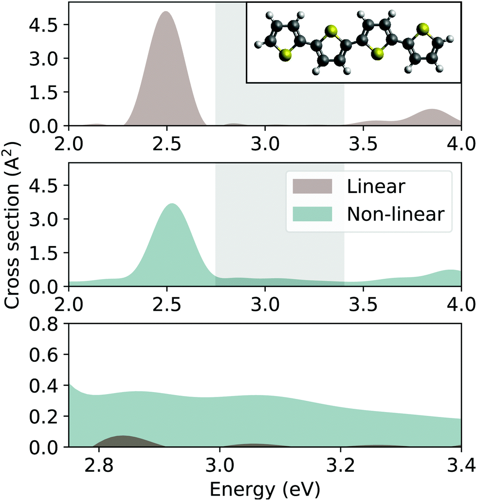 | ||
| Fig. 1 Absorption cross section of the 4T oligomer computed from real-time TDDFT using the non-linear impulse approach from ref. 55 in the linear regime (top panel) and in the nonlinear one (middle panel). The grey shaded area marks the optical limiting region for which the linear and nonlinear cross sections are overlaid on the bottom panel. Inset: 4T molecule in the ball-and-stick representation, with C atoms in grey, S atoms in yellow, and H atoms in white. | ||
The results presented in Fig. 1 demonstrate the general applicability of the non-linear impulse approach in the framework of real-time TDDFT, to calculate the nonlinear optical absorption of molecules and atomic cluster, and predict intriguing properties such as optical limiting. However, from these results, we cannot say much about the origin of this behavior, and a number of open questions remain. For example: (i) Why do the peaks in linear absorption spectrum loose oscillator strength and what determines the corresponding amount?; (ii) What is the fundamental physical origin behind the increasing absorption in the transparent window in linear regime? (iii) Is it possible to relate the optical response obtained in the adopted non-perturbative approach with that given by perturbation theory?
In order to overcome this troublesome lack of understanding, it is necessary to take a step back and apply the proposed non-perturbative approach to systems that we are able to tackle via accurate ab initio methodology or to restrict ourselves to model systems that can be solved exactly. In this way, we can look at the behavior of interacting quantities which are not directly accessible via TDDFT (which directly provides us the time-dependent particle density only). Moreover, we can focus on the output of the methodology – i.e., probing the systems via instantaneous, intense electrical fields – disentangled from the effects of an approximation of TDDFT or other numerical intricacies which may be met for complex systems. In return, the gained insight obtained with this strategy can provide valuable information to consciously and effectively embed this method in real-time TDDFT simulations, in order to exploit its full potential.
3 Absorption cross section in the instantaneous impulsive limit
Let us consider a system of N interacting electrons subject to a time-dependent classical electric field in the dipole approximation, described by the Hamiltonian Ĥ(t) = Ĥ0 −![[d with combining circumflex]](https://www.rsc.org/images/entities/i_char_0064_0302.gif) μ
μ![[scr E, script letter E]](https://www.rsc.org/images/entities/char_e140.gif) μ(t) (summation over repeated indices is understood), where Ĥ0 includes the ordinary electron–nuclei and electron–electron Coulomb interaction,
μ(t) (summation over repeated indices is understood), where Ĥ0 includes the ordinary electron–nuclei and electron–electron Coulomb interaction,  is the electric dipole operator with
 ![[r with combining circumflex]](https://www.rsc.org/images/entities/i_char_0072_0302.gif) iμ, and μ = x,y,z is the μ-th component of the position operator of the i-th electron. Spin–orbit coupling is neglected. We aim to describe the light absorption process in the case of an extremely short pulse, i.e. in the limit of a Dirac-delta time-dependence
iμ, and μ = x,y,z is the μ-th component of the position operator of the i-th electron. Spin–orbit coupling is neglected. We aim to describe the light absorption process in the case of an extremely short pulse, i.e. in the limit of a Dirac-delta time-dependence| μ(t) = κμδ(t). | (1) |
 . Here, we focus our analysis on absorption at equilibrium, i.e., we suppose that the system is in its ground state at t < 0, namely |Ψ(t < 0)〉 = |Ψ0〉e−iE0t. For a description of the out-of-equilibrium absorption processes, as in the case of time-resolved absorption spectroscopy, further analysis is required.105
For t > 0, the solution of the time-dependent Schrödinger equation |Ψ(t)〉 can be projected onto the eigenstates {|Ψi〉} of Ĥ0 as
 | (2) |
| ci = 〈Ψi|e−iμκμ|Ψ0〉. | (3) |
μ|Ψ(t)〉 for such a system is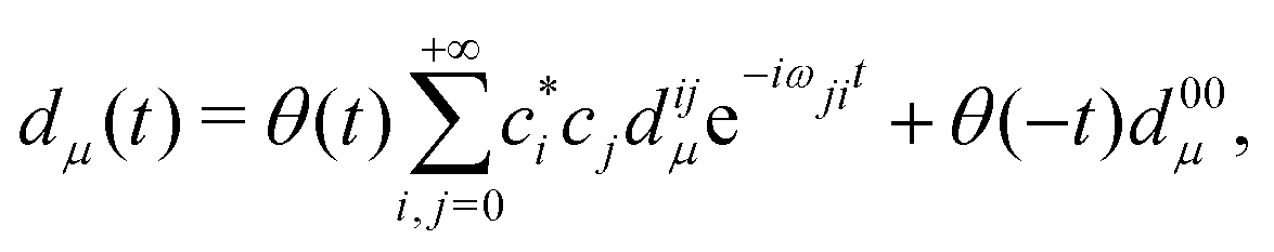 | (4) |
μ|Ψj〉 are the dipole matrix elements, d00μ is the ground state dipole, and ωji = Ej − Ei is the energy difference between the j-th and i-th eigenstates of the unperturbed Hamiltonian Ĥ0.
We now want to employ the explicit shape for the dipole moment in eqn (4) in order to calculate the absorption cross section
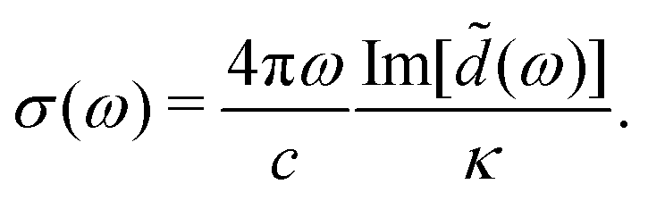
 | (5) |
By Fourier transforming eqn (4), substituting it into eqn (5), and assuming, for sake of simplicity, that the system is centrosymmetric (i.e., d00μ = 0), we obtain
 | (6) |
μκμ)|Ψj〉, Sij ≡ 〈Ψi|sin(μκμ)|Ψj〉, and M(n)ij ≡ 〈Ψi|(μκμ)n|Ψj〉, with M(1)ij ≡ Mij. Eqn (6), derived in the ESI,† can be used to describe any centrosymmetric system, or an ensemble of non-centrosymmetric objects randomly oriented with respect to the direction of the electric field. Since the ensemble-averaged optical response is centrosymmetric regardless of the point symmetry of the individual molecules, the average cross section is obtained by sampling and averaging the responses to impulses with different polarization directions.
In order to highlight the nonlinear character of the cross section, we compute the linear absorption cross section σ(1)(ω) by approximating the matrix elements in eqn (6) up to the first order in κ. We can physically define the concept of “small κ” since the magnitude of the dipole is limited by the spatial extension R of the system. For molecular systems with R ≈ (1 − 100) Bohr, μκμ ≪ 1 when κ ≪ 1/R. Therefore, κ ≈ 10−3 Bohr−1 is suitable to define a weak field in the impulsive limit.66 Since sin(μκμ) ≈ μκμ and cos(μκμ) ≈ ![[1 with combining circumflex]](https://www.rsc.org/images/entities/char_0031_0302.gif) , we have
, we have
 | (7) |
For small κ (in the above-mentioned sense), eqn (7) provides a good approximation for eqn (6).
While in the linear regime the resonances in the cross section are only found at ω = ωj0 ≡ Ej − E0, in eqn (6) the resonances occur at ω = ωji ≡ Ej − Ei; i.e., for the energy of the incoming light equating the energy difference between any pair of eigenstates of the unperturbed Hamiltonian Ĥ0. This is sketched in Fig. 2, in which black arrows indicate ground-state absorption (GSA), as given by eqn (7), and red arrows denote excited-state absorption (ESA), as given by eqn (6). ESA, in practice, can occur when one or more excited states of the unperturbed system are populated by a laser.
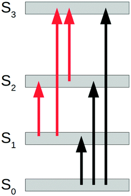 | ||
| Fig. 2 Sketch of ground-state (black) and excited-state (red) excitations in the singlet manifold. Excited-state excitations involve transitions between excited states and are activated in the nonlinear regime described by eqn (6). Ground-state absorption is described by the ordinary linear cross section in eqn (7). | ||
Eqn (6) and (7) share the same dipole parity selection rule, as they include the same matrix elements Mij, with i = 0 in eqn (7). However, while states with the same parity as the ground state cannot be populated in the linear regime, they can be populated in the nonlinear regime through ESA. Further, the individual contributions to eqn (6) vanish for all the states i with either C0i = 0, or S0i = 0. In the next section, we exploit this fact to determine the set of transitions that build up the ESA at different field strengths. Also note that in eqn (6)σ(ω) satisfies the Thomas–Reiche–Kuhn sum rule in the form
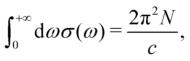 | (8) |
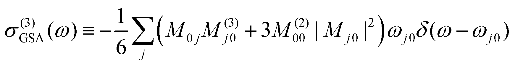
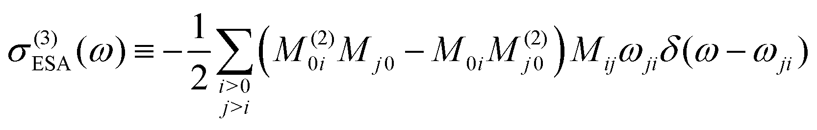
The perturbative analysis can be carried on by further expanding eqn (6) in powers of κ. The second-order term, like all subsequent terms of even order, vanishes because we assumed inversion symmetry. The third-order term is
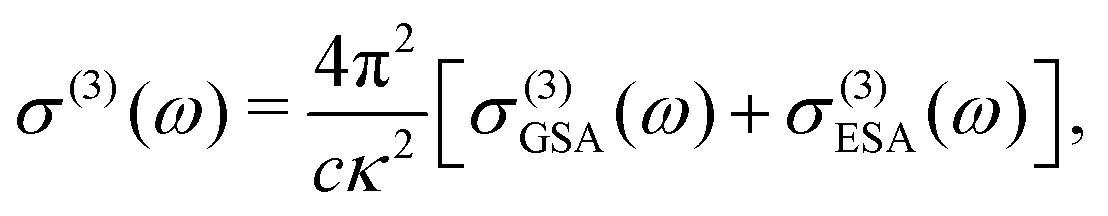 | (9) |
 | (10) |
 | (11) |
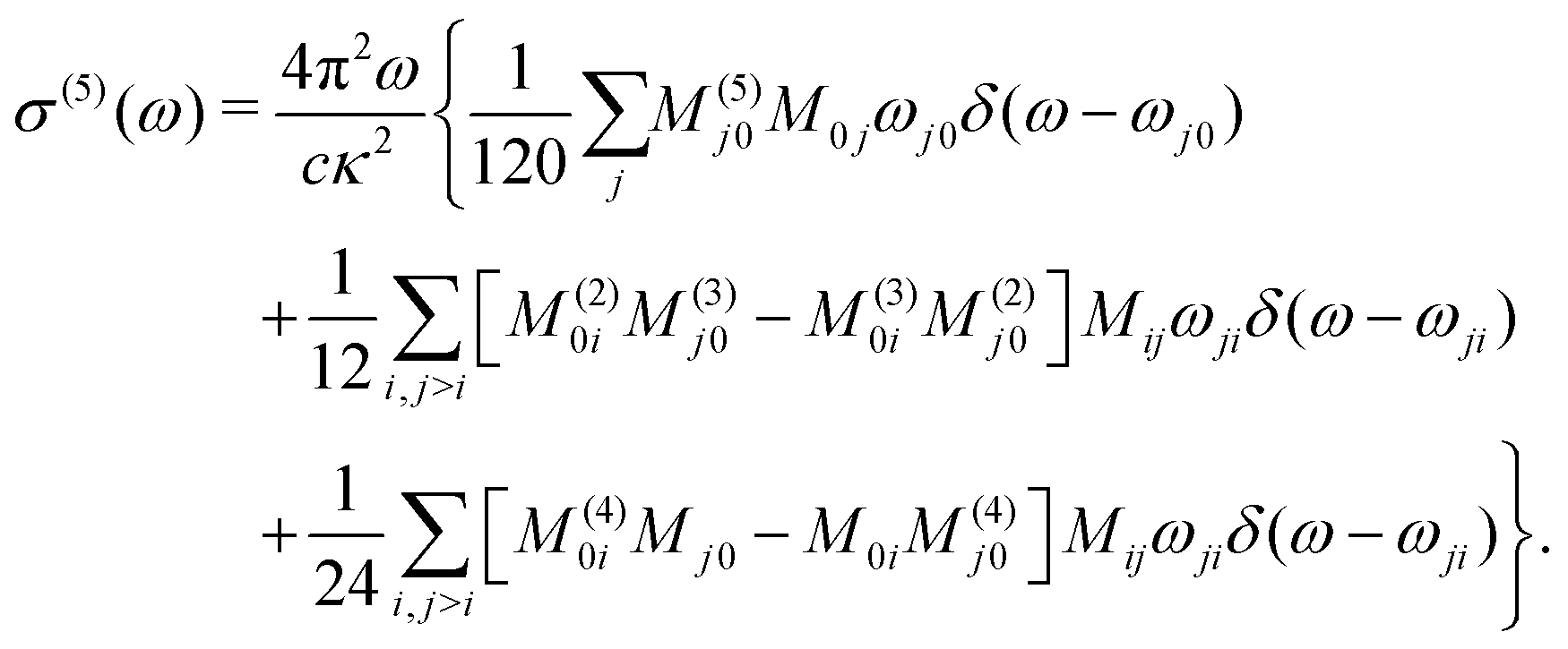 | (12) |
Even if eqn (9) also accounts for two-photon processes, the impulsive field has a fixed frequency dependence. Therefore, it cannot predict spectra obtained by means of non-impulsive field shapes. On the other hand, eqn (9) allows us to directly identify the spectral weight due to specific set of transitions at a common resonance. Consequently, accessing σ(ω) with an instantaneous impulse is most useful to describe ESA (which is fluence dependent) but it is not suitable for a full description of two-photon absorption (which is irradiance dependent).106
Obviously, the impulse response obtained from real-time propagation of the quantum state is intrinsically non perturbative: namely, from the evolved quantum state we compute dμ(t) = 〈Ψ(t)|μ|Ψ(t)〉 and, thus, the Fourier transform dμ(ω) can be readily obtained. The latter can be finally used in eqn (5). According to the previous analysis, the approach captures ESA at all the possible resonances. Furthermore, because dμ(t) can be expressed in terms of the particle density, 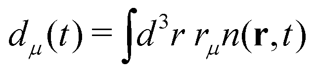 , the procedure based on real-time propagation can be readily implemented in any code that solves the time-dependent Kohn–Sham equations without the need for the explicit knowledge of the many-body wave function. Thus, large systems can be tackled efficiently within TDDFT approximations.55
Before moving to the next section – where the numerical application to a model system and the related careful analytical investigation allow to gain further insights – we emphasize that spin–orbit coupling and magnetic fields are not included in our considerations. We work under the assumption that the ground state is a spin singlet, thus, both expressions in eqn (6) and eqn (7) allow transitions only within the manifold of singlet excited states. Studying the absorption of excited states with different spin multiplicity is important, for example, to account for inter-system crossing107 which can occur in optical limiting processes. Formally, this would require to use spin-dependent impulses.108,109
4 Analysis of nonlinear absorption in a 1D model system
Here, we scrutinize the information that can be retrieved by the “real-time impulsive method” on the cross section of an interacting system beyond the linear regime. Our choice to work at the level of a simple model system, instead of a real molecule, allows us to avoid from the outset the challenge of the typical approximations of state-of-the-art TDDFT. Below, we also compare results from the perturbative expressions derived in the previous section with the computed non-perturbative solution obtained by directly time-evolving the many-body sate.The considered system consists of two interacting electrons confined in a one-dimensional segment by a potential well of infinite depth (hereafter 1DW). The unperturbed Hamiltonian of the 1DW is
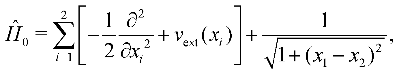 | (13) |
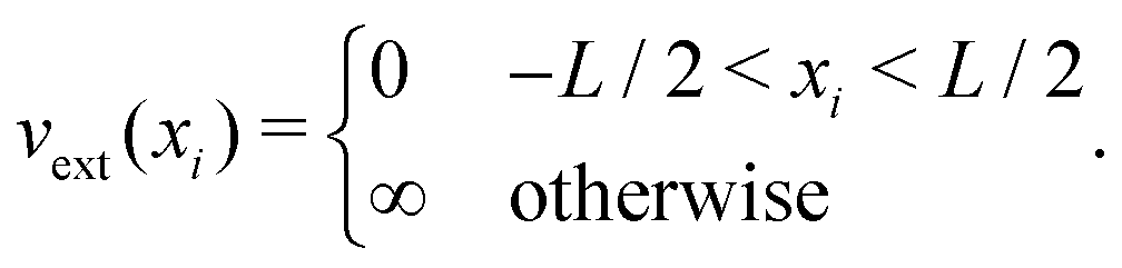 | (14) |
The time-dependent polarization is calculated as d(t) = 〈Ψ(t)||Ψ(t)〉 and its Fourier transform ![[d with combining tilde]](https://www.rsc.org/images/entities/i_char_0064_0303.gif) (ω) enters the absorption cross section
(ω) enters the absorption cross section
 | (15) |
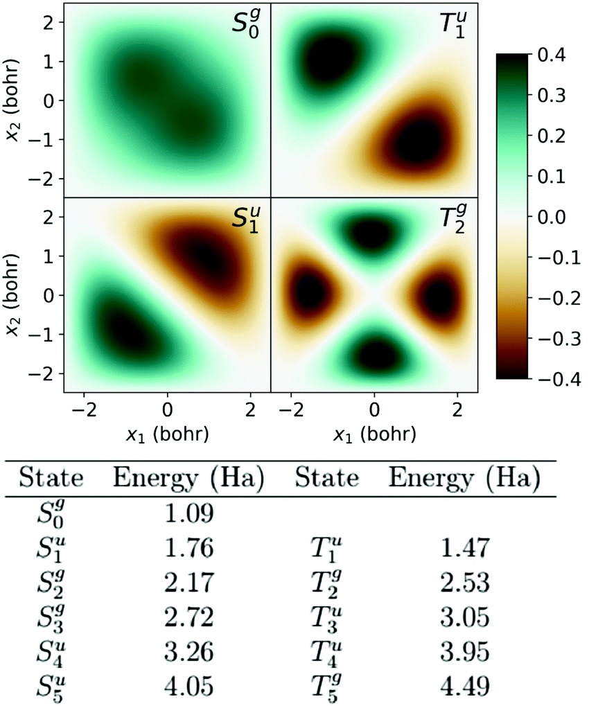 | ||
| Fig. 3 Plot: Eigenstates depicted in the configuration space x1−x2 (left) of the unperturbed system of two electrons in a 1D potential well of infinite depth (eqn (13)). The states are labeled as Sg/ui, where S indicates the spin state (singlet S or triplet T), i the order in energy within the spin channel, and g/u the parity with respect to inversion of the coordinates. Colorbar units are Bohr−1. Table: Eigenvalues of the first five eigenvectors of the unperturbed Hamiltonian in eqn (13). | ||
The linear and nonlinear absorption spectra of the 1DW obtained by applying an electric field impulse with κ = 0.01 Bohr−1 and 0.80 Bohr−1, respectively, are shown in Fig. 4. Given the well length and the spacing of the ground-state eigenvalues, the field corresponding to κ ≤ 0.02 Bohr−1 can be considered weak. The resulting cross sections show an intrinsic broadening of 0.04 Ha due to the finite duration of the time propagation.
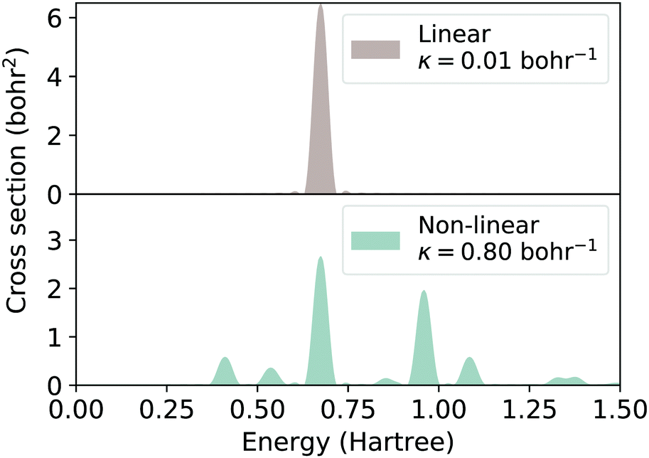 | ||
| Fig. 4 Comparison between the linear and nonlinear absorption spectra of a 1D square potential well containing two electrons (1DW). The linear absorption spectrum (upper panel) is obtained by applying an impulsive electric field with strength κ = 0.01 Bohr−1 (weak-field regime). The nonlinear absorption spectrum (lower panel) is obtained by applying an electric field with strength κ = 0.80 Bohr−1 (strong field regime). | ||
In the upper panel of Fig. 4 the linear spectrum shows a single maximum at 0.67 Ha, corresponding to the Sg0 → Su1 transition. In contrast, the nonlinear absorption cross section features several peaks spread over the range (0.4–1.4) Ha, namely at lower and higher energies with respect to the excitation in the linear regime. In the nonlinear regime, the maximum corresponding to the Sg0 → Su1 transition at 0.67 Ha is not suppressed but its spectral weight is approximately halved.
To analyze the transitions involved in the nonlinear cross section, in Fig. 5 we consider separately the contributions of three components, namely σS0(ω), σS1(ω), and σ{Sm}(ω), with m ≥ 2. The first and second components account for the absorption from the ground state and from the first excited state, while the third one includes the contributions from all higher excited states. These components are calculated from eqn (6) evaluating the sums up to the first 100 eigenstates of Ĥ0. Convergence is ensured by the sum rule in eqn (8). Dirac deltas in eqn (6) are broadened in order to match the peak width of the cross sections obtained from the solution of the time-dependent Schrödinger equation.
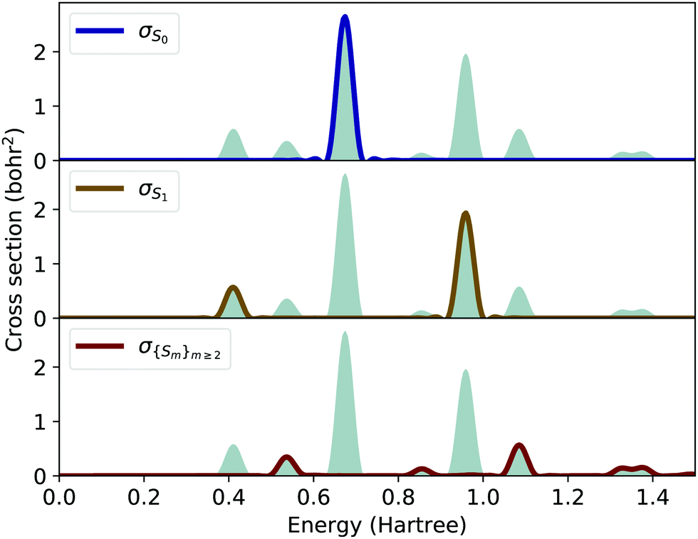 | ||
| Fig. 5 Nonlinear absorption cross section of the 1DW subject to a strong electric field impulse with κ = 0.80 Bohr−1. The cross section is split into ground-state absorption (blue curve), first excited-state absorption (yellow curve) and absorption from higher excited states (red curve). | ||
The component σS0(ω) (top panel of Fig. 5) includes the same contribution as the linear cross section, Sg0 → Su1 (see top panel of Fig. 4). Therefore, the additional peaks in the lower panel of Fig. 4 result from ESA. In particular, the two peaks at 0.41 Ha and 0.96 Ha (see middle panel of Fig. 5) are due to the absorption from the first excited state (Su1) and involve the transitions to gerade excited states Su1 → Sg2 and Su1 → Sg3, respectively. Simply based on symmetry, the excited states Sg2 and Sg3 cannot be reached from the ground state Sg0. By inspecting the bottom panel of Fig. 5, we notice that the higher-order contributions to the absorption consist of a number of weak peaks below and above the maximum at 0.67 Ha. For example, the maximum at about 1.1 Ha corresponds to the transition Sg2 → Su4.
To gain further understanding on the information provided by the non-perturbative approach presented so far, it is interesting to inspect the variation of the relative weights of GSA and ESA as a function of the field strength. These contributions are quantified by
 | (16) |
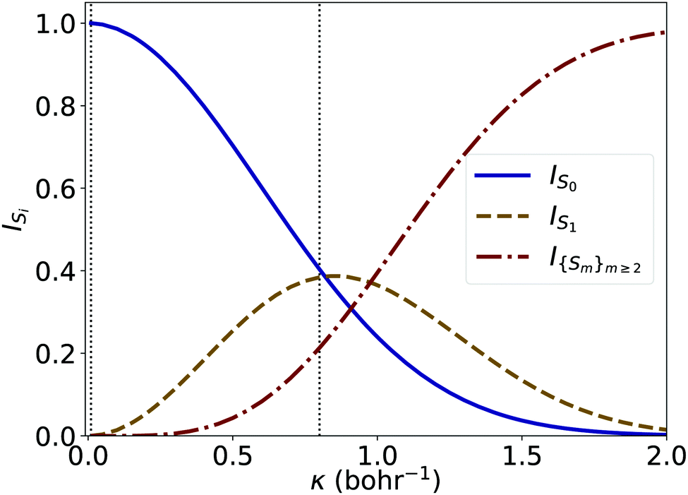 | ||
| Fig. 6 Normalized weights [see eqn (16)] of the three components of the absorption cross section given in Fig. 5 as a function of the strength of the electric field impulse κ. The dashed vertical bars correspond to the values of κ used in Fig. 4. | ||
We complete our analysis by considering the perturbative expansion of the nonlinear absorption cross section, as discussed in Section 3. The perturbative terms σ(1)(ω), σ(3)(ω), and σ(5)(ω) are shown in on the left panel of Fig. 7. They are computed from eqn (7), (9) and (12). The cross section σ(ω) calculated with the impulse response method for κ = 0.80 Bohr−1 is also shown for reference. For comparison, on the right panel of Fig. 7 we show the perturbative contribution summed up to the indicated order.
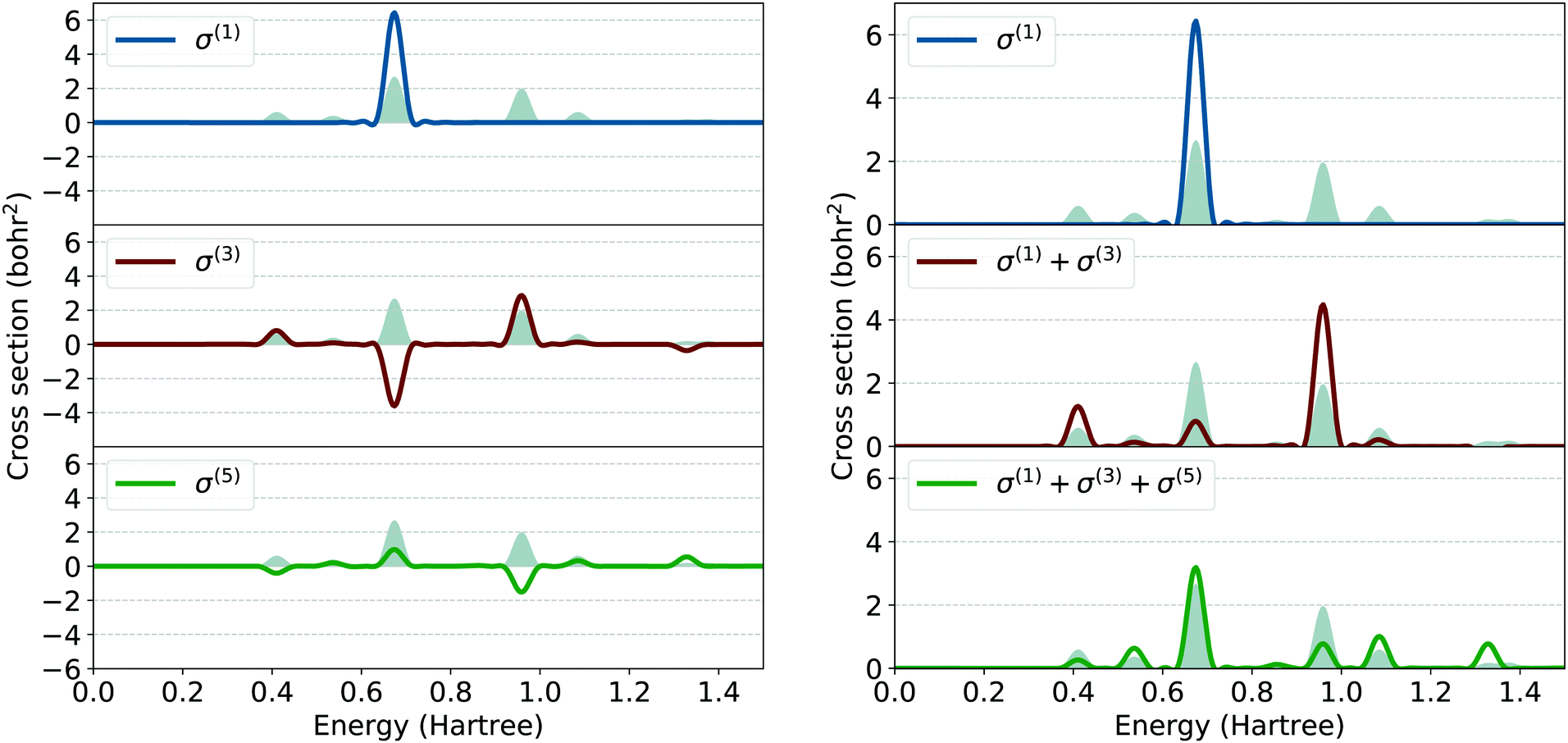 | ||
| Fig. 7 Left panel: Perturbative components σ(1), σ(3) and σ(5) (Eqn (7), (9) and (12) respectively) of the nonlinear absorption cross section the 1DW subject to the electric field impulse κ = 0.80 Bohr−1. For reference, the total cross section (eqn (6)), also shown in the bottom panel of Fig. 4, is plotted as shaded area in the background of each panel. Right panel: Summation of the first five non-zero terms in the perturbation series compared to the full non-perturbative result (shaded grey area). | ||
The first-order cross section σ(1)(ω) assumes only positive values and contributes only to the maximum at 0.67 Ha. The first nonlinear non-vanishing component of the cross section, which thus accounts for ESA processes, is the third-order one, σ(3), which assumes both positive and negative values. A pronounced peak with negative strength is found at 0.67 Ha and corresponds to the third-order correction of the ground-state transition Sg0 → Su1. This term cancels out almost completely the contribution from σ(1) at the same energy. Maxima with positive intensities appear at about 0.4 Ha and 1.0 Ha.
However, the contribution of σ(3) alone is not sufficient to describe the nonlinear excitations in the 1DW – see Fig. 7, left panel, middle graph. For this purpose, it is necessary to include at least also the contributions from the fifth-order cross section, σ(5). This term has maxima and minima at the same energy as those of σ(3) but with intensities of opposite sign. In particular, the peak at 0.67 Ha is positive and overlaps almost perfectly with the one in the impulse cross section shown in the background. Minima are found at approximately 0.4 Ha and 1.0 Ha, at the same energies where σ(3) exhibits maxima. The absolute values of the corresponding intensities are very similar, suggesting that these contributions should cancel out. We stress the fact that summing up the perturbative contributions of σ up to the fifth order is still not sufficient to match the non-perturbative result. Even assuming that the perturbative series is within its convergence radius (which is not trivially granted), Fig. 7 shows that for large values of κ the terms of the series tend to have alternating sign contributions, which explains the observed difficulties in the convergence.
5 Discussion
Before moving to our general conclusions, we look back at the linear and nonlinear absorption spectra computed for the 4T molecule (see Fig. 1). Although the spectral region considered in that case was significantly narrower in energy than the one examined in the 1DW model (see Fig. 4), we can recognize some common features. First and foremost, with the exactly solvable system, we have clarified that the oscillator strength arising above the absorption onset in the linear regime stems from excited-state absorption that can be associated to specific contributions in the perturbative expansion of the total cross section (see Fig. 7). Also the loss of spectral weight of the first peak in the nonlinear regime is explained as a renormalization due to the high-order contributions to the cross section. Finally, nonlinear effects are responsible for the enhanced absorption below the linear absorption onset.We stress that the impulse approach cannot access the dependence of the spectrum on the pulse shape. Therefore, it cannot be exploited, as it is, to study processes such as two-photon absorption or ultrafast transients. It is not suitable either to investigate those cases in which hysteresis loops or other memory-dependent phenomena are important. However, for cases in which the interest in optical nonlinearities is not restricted to wave mixing at a predefined order, or at a single frequency, the computation of observables from real-time propagation in the nonlinear impulsive excitation regime is particularly useful to perform a wide-band quick check for the presence of non-linear effects outperforming the ordinary approach based on perturbation theory. In fact this technique does not make use of unoccupied states, which implies a number of computational advantages: it is not affected by the convergence issues of perturbative methods or by the choice of an active space; it is equally stable on and off-resonance (at difference, for example, with Sternheimer's method28); its sensitivity is controlled by the same parameters as a linear propagation (namely, time step and total propagation time); it is easily scalable; it is easily integrated with a nuclear dynamics scheme.
These features render this method an ideal tool to scan materials for potential interesting non-linearities induced by excited state absorption such as reverse saturable absorption, optical switching, and optical limiting.
6 Conclusions and outlook
In conclusion, we have shown that the time-evolution of many-electron systems induced by an electric field in the instantaneous limit is an effective tool for investigating computationally fluence-dependent nonlinear optical properties. It works well also for those cases in which the convergence of the perturbative expansions of the cross sections is challenging. Specifically, we have shown that the impulsive method provides relevant information about the steady-state absorption of time-invariant systems in which the nonlinear effects manifest themselves merely as a function of the field fluence.One of the main advantages of the impulse technique is that the nonlinear absorption cross section is promptly obtained at computational costs that are comparable with those needed for linear response in real time and certainly much lower with respect to conventional perturbative approaches. This method is deliberately designed to take advantage of an infinite bandwidth excitation to search for optical nonlinearities of a system. Its application in the framework of real-time TDDFT to a free-base phthalocyanine molecule demonstrated that the outcome of optical limiting experiments based on the Z-scan technique113 can be successfully reproduced.55
We envision additional theoretical work in the near future that systematically analyzes the impact of approximations of TDDFT also beyond the linear regime. We are confident that these developments will provide the community with novel, powerful computational tools that are able to complement emerging experimental directions in ultrafast spectroscopy.114–116
Conflicts of interest
There are no conflicts to declare.Acknowledgements
A. G. acknowledges financial support from the German Academic Exchange Service (DAAD) grant n. 57440917 and from HPC Europa 3 grant no HPC17AS2HO. C. C. appreciates funding from the German Research Foundation (DFG), Project number 182087777 – SFB 951, from the German Federal Ministry of Education and Research (Professorinnenprogramm III) as well as from the State of Lower Saxony (Professorinnen für Niedersachsen). Computational resources provided by the North-German Supercomputing Alliance (HLRN), project bep00060, and by the High Performance Computing Center Stuttgart (HLRS). S. P. acknowledges financial support through MIUR PRIN Grant No. 2017RKWTMY. C. A. R. acknowledges support from MIUR PRIN Grant No. 201795SBA3.References
- P. A. Franken, A. E. Hill, C. W. Peters and G. Weinreich, Phys. Rev. Lett., 1961, 7, 118–119 CrossRef.
- T. Damm, M. Kaschke, F. Noack and B. Wilhelmi, Opt. Lett., 1985, 10, 176–178 CrossRef CAS PubMed.
- M. D. Perry and G. Mourou, Science, 1994, 264, 917–924 CrossRef CAS PubMed.
- R. W. Boyd, Nonlinear Optics, Third Edition, Academic Press, Inc., USA, 3rd edn, 2008 Search PubMed.
- S. Tretiak and V. Chernyak, J. Chem. Phys., 2003, 119, 8809–8823 CrossRef CAS.
- B. I. Grimberg, V. V. Lozovoy, M. Dantus and S. Mukamel, J. Phys. Chem. A, 2002, 106, 697–718 CrossRef CAS.
- I. Tunell, Z. Rinkevicius, O. Vahtras, P. Sałek, T. Helgaker and H. Ågren, J. Chem. Phys., 2003, 119, 11024–11034 CrossRef CAS.
- B. Jansik, P. Sałek, D. Jonsson, O. Vahtras and H. Ågren, J. Chem. Phys., 2005, 122, 054107 CrossRef PubMed.
- S. J. A. van Gisbergen, J. G. Snijders and E. J. Baerends, J. Chem. Phys., 1998, 109, 10644–10656 CrossRef CAS.
- M. de Wergifosse and S. Grimme, J. Chem. Phys., 2018, 149, 024108 CrossRef PubMed.
- H. Hait Heinze, F. Della Sala and A. Görling, J. Chem. Phys., 2002, 116, 9624–9640 CrossRef CAS.
- J. Henriksson, T. Saue and P. Norman, J. Chem. Phys., 2008, 128, 024105 CrossRef PubMed.
- G. Senatore and K. R. Subbaswamy, Phys. Rev. A: At., Mol., Opt. Phys., 1987, 35, 2440–2447 CrossRef CAS PubMed.
- J.-I. Iwata, K. Yabana and G. F. Bertsch, J. Chem. Phys., 2001, 115, 8773–8783 CrossRef CAS.
- A. Ye and J. Autschbach, J. Chem. Phys., 2006, 125, 234101 CrossRef PubMed.
- D. R. Kanis, M. A. Ratner and T. J. Marks, J. Am. Chem. Soc., 1992, 114, 10338–10357 CrossRef CAS.
- O. Quinet, B. Champagne and B. Kirtman, J. Comput. Chem., 2001, 22, 1920–1932 CrossRef CAS.
- O. Quinet and B. Champagne, Int. J. Quantum Chem., 2001, 85, 463–468 CrossRef CAS.
- O. Quinet and B. Champagne, J. Chem. Phys., 2002, 117, 2481–2488 CrossRef CAS.
- D. Jonsson, P. Norman and H. Ågren, J. Chem. Phys., 1996, 105, 6401–6419 CrossRef CAS.
- O. Berman and S. Mukamel, Phys. Rev. A: At., Mol., Opt. Phys., 2003, 67, 042503 CrossRef.
- H. Hettema, H. J. A. Jensen, P. Jo/rgensen and J. Olsen, J. Chem. Phys., 1992, 97, 1174–1190 CrossRef CAS.
- A. Ye, S. Patchkovskii and J. Autschbach, J. Chem. Phys., 2007, 127, 074104 CrossRef PubMed.
- P. Sałek, O. Vahtras, T. Helgaker and H. Ågren, J. Chem. Phys., 2002, 117, 9630–9645 CrossRef.
- Z. Rinkevicius, P. C. Jha, C. I. Oprea, O. Vahtras and H. Ågren, J. Chem. Phys., 2007, 127, 114101 CrossRef PubMed.
- P. Elliott, S. Goldson, C. Canahui and N. T. Maitra, Chem. Phys., 2011, 391, 110–119 CrossRef CAS.
- S. M. Parker, D. Rappoport and F. Furche, J. Chem. Theory Comput., 2018, 14, 807–819 CrossRef CAS PubMed.
- X. Andrade, S. Botti, M. A. L. Marques and A. Rubio, J. Chem. Phys., 2007, 126, 184106 CrossRef PubMed.
- E. Luppi, H. Hübener and V. Véniard, Phys. Rev. B: Condens. Matter Mater. Phys., 2010, 82, 235201 CrossRef.
- J. L. P. Hughes and J. E. Sipe, Phys. Rev. B: Condens. Matter Mater. Phys., 1996, 53, 10751–10763 CrossRef CAS PubMed.
- M. Veithen, X. Gonze and P. Ghosez, Phys. Rev. B: Condens. Matter Mater. Phys., 2005, 71, 125107 CrossRef.
- L. Prussel and V. Véniard, Phys. Rev. B, 2018, 97, 205201 CrossRef CAS.
- D. H. Friese, M. T. P. Beerepoot, M. Ringholm and K. Ruud, J. Chem. Theory Comput., 2015, 11, 1129–1144 CrossRef CAS PubMed.
- D. H. Friese, R. Bast and K. Ruud, ACS Photonics, 2015, 2, 572–577 CrossRef CAS PubMed.
- T. Brabec and F. Krausz, Rev. Mod. Phys., 2000, 72, 545–591 CrossRef CAS.
- E. Lorin, M. Lytova, A. Memarian and A. D. Bandrauk, J. Phys. A: Math. Theor., 2015, 48, 105201 CrossRef.
- R. L. Peterson, Rev. Mod. Phys., 1967, 39, 69–77 CrossRef CAS.
- I. Safi and P. Joyez, Phys. Rev. B: Condens. Matter Mater. Phys., 2011, 84, 205129 CrossRef.
- V. V. Strelkov, Phys. Rev. A, 2016, 93, 053812 CrossRef.
- J. J. Goings, P. J. Lestrange and X. Li, Wiley Interdiscip. Rev.: Comput. Mol. Sci., 2018, 8, 1–19 Search PubMed.
- M. R. Provorse and C. M. Isborn, Int. J. Quantum Chem., 2016, 116, 739–749 CrossRef CAS.
- D. Cho, J. R. Rouxel, M. Kowalewski, P. Saurabh, J. Y. Lee and S. Mukamel, J. Phys. Chem. Lett., 2018, 9, 1072–1078 CrossRef CAS PubMed.
- F. Ding, B. E. Van Kuiken, B. E. Eichinger and X. Li, J. Chem. Phys., 2013, 138, 064104 CrossRef PubMed.
- J. Mattiat and S. Luber, J. Chem. Phys., 2018, 149, 174108 CrossRef PubMed.
- E. Penka Fowe and A. D. Bandrauk, Phys. Rev. A: At., Mol., Opt. Phys., 2011, 84, 035402 CrossRef.
- E. Luppi and M. Head-Gordon, Mol. Phys., 2012, 110, 909–923 CrossRef CAS.
- T. S. Nguyen, J. H. Koh, S. Lefelhocz and J. Parkhill, J. Phys. Chem. Lett., 2016, 7, 1590–1595 CrossRef CAS PubMed.
- N. Tancogne-Dejean, O. D. Mücke, F. X. Kärtner and A. Rubio, Phys. Rev. Lett., 2017, 118, 087403 CrossRef PubMed.
- S. A. Sato, K. Yabana, Y. Shinohara, T. Otobe, K.-M. Lee and G. F. Bertsch, Phys. Rev. B: Condens. Matter Mater. Phys., 2015, 92, 205413 CrossRef.
- C. A. Ullrich, Time-dependent density-functional theory: concepts and applications, Oxford University Press, Oxford, 2011 Search PubMed.
- M. A. Marques, N. T. Maitra, F. M. Nogueira, E. K. U. Gross and A. Rubio, Fundamentals of Time-Dependent Density Functional Theory, Springer, Berlin, Heidelberg, 2012 Search PubMed.
- Y. Takimoto, F. D. Vila and J. J. Rehr, J. Chem. Phys., 2007, 127, 154114 CrossRef CAS PubMed.
- C. Attaccalite and M. Grüning, Phys. Rev. B: Condens. Matter Mater. Phys., 2013, 88, 1–10 CrossRef.
- M. Uemoto, Y. Kuwabara, S. A. Sato and K. Yabana, J. Chem. Phys., 2019, 150, 094101 CrossRef PubMed.
- C. Cocchi, D. Prezzi, A. Ruini, E. Molinari and C. A. Rozzi, Phys. Rev. Lett., 2014, 112, 1–5 CrossRef PubMed.
- J. L. Alonso, X. Andrade, P. Echenique, F. Falceto, D. Prada-Gracia and A. Rubio, Phys. Rev. Lett., 2008, 101, 096403 CrossRef CAS PubMed.
- S. M. Falke, C. A. Rozzi, D. Brida, M. Maiuri, M. Amato, E. Sommer, A. De Sio, A. Rubio, G. Cerullo, E. Molinari and C. Lienau, Science, 2014, 344, 1001–1005 CrossRef CAS PubMed.
- S. Pittalis, A. Delgado, J. Robin, L. Freimuth, J. Christoffers, C. Lienau and C. A. Rozzi, Adv. Funct. Mater., 2015, 25, 2047–2053 CrossRef CAS.
- C. A. Rozzi, F. Troiani and I. Tavernelli, J. Phys.: Condens. Matter, 2017, 30, 013002 CrossRef PubMed.
- C. A. Rozzi and S. Pittalis, Handbook of Materials Modeling, Springer International Publishing, Cham, 2018, pp. 1–19 Search PubMed.
- A. Yamada and K. Yabana, Phys. Rev. B, 2019, 99, 245103 CrossRef CAS.
- M. Jacobs, J. Krumland, A. M. Valencia, H. Wang, M. Rossi and C. Cocchi, Adv. Phys.: X, 2020, 5, 1749883 CAS.
- J. Krumland, A. M. Valencia, S. Pittalis, C. A. Rozzi and C. Cocchi, J. Chem. Phys., 2020, 153, 054106 CrossRef CAS PubMed.
- J. Yuen-Zhou, D. G. Tempel, C. A. Rodríguez-Rosario and A. Aspuru-Guzik, Phys. Rev. Lett., 2010, 104, 043001 CrossRef PubMed.
- R. W. Newcomb, Proc. IEEE, 1963, 51, 1157–1158 Search PubMed.
- K. Yabana and G. F. Bertsch, Phys. Rev. B: Condens. Matter Mater. Phys., 1996, 54, 4484–4487 CrossRef CAS PubMed.
- D. Dini, M. J. Calvete and M. Hanack, Chem. Rev., 2016, 116, 13043–13233 CrossRef CAS PubMed.
- Y.-P. Sun and J. E. Riggs, Int. Rev. Phys. Chem., 1999, 18, 43–90 Search PubMed.
- Q. Miao, Z. Sang, R. Song, M. Liang, Q. Liu, E. Sun and Y. Xu, J. Photochem. Photobiol., A, 2019, 385, 112087 CrossRef CAS.
- M. de Wergifosse and S. Grimme, J. Chem. Phys., 2019, 150, 094112 CrossRef PubMed.
- S. A. Fischer, C. J. Cramer and N. Govind, J. Chem. Theory Comput., 2015, 11, 4294–4303 CrossRef CAS PubMed.
- S. A. Fischer, C. J. Cramer and N. Govind, J. Phys. Chem. Lett., 2016, 7, 1387–1391 CrossRef CAS PubMed.
- D. N. Bowman, J. C. Asher, S. A. Fischer, C. J. Cramer and N. Govind, Phys. Chem. Chem. Phys., 2017, 19, 27452–27462 RSC.
- S. Ghosh, J. C. Asher, L. Gagliardi, C. J. Cramer and N. Govind, J. Chem. Phys., 2019, 150, 104103 CrossRef PubMed.
- P. Elliott and N. T. Maitra, Phys. Rev. A: At., Mol., Opt. Phys., 2012, 85, 052510 CrossRef.
- M. A. Mosquera, L. X. Chen, M. A. Ratner and G. C. Schatz, J. Chem. Phys., 2016, 144, 204105 CrossRef PubMed.
- X. Sheng, H. Zhu, K. Yin, J. Chen, J. Wang, C. Wang, J. Shao and F. Chen, J. Phys. Chem. C, 2020, 124, 4693–4700 CrossRef CAS.
- Q. Bellier, N. S. Makarov, P.-A. Bouit, S. Rigaut, K. Kamada, P. Feneyrou, G. Berginc, O. Maury, J. W. Perry and C. Andraud, Phys. Chem. Chem. Phys., 2012, 14, 15299–15307 RSC.
- S. A. Fischer, C. J. Cramer and N. Govind, J. Phys. Chem. Lett., 2016, 7, 1387–1391 CrossRef CAS PubMed.
- J. I. Fuks and N. T. Maitra, Phys. Chem. Chem. Phys., 2014, 16, 14504–14513 RSC.
- K. Luo, P. Elliott and N. T. Maitra, Phys. Rev. A: At., Mol., Opt. Phys., 2013, 88, 042508 CrossRef.
- J. I. Fuks, P. Elliott, A. Rubio and N. T. Maitra, J. Phys. Chem. Lett., 2013, 4, 735–739 CrossRef CAS PubMed.
- P. Elliott, J. I. Fuks, A. Rubio and N. T. Maitra, Phys. Rev. Lett., 2012, 109, 266404 CrossRef CAS PubMed.
- N. T. Maitra, J. Chem. Phys., 2005, 122, 234104 CrossRef PubMed.
- N. Mardirossian and M. Head-Gordon, Mol. Phys., 2017, 115, 2315–2372 CrossRef CAS.
- I. Salzmann, G. Heimel, M. Oehzelt, S. Winkler and N. Koch, Acc. Chem. Res., 2016, 49, 370–378 CrossRef CAS PubMed.
- L. Zhu, E.-G. Kim, Y. Yi and J.-L. Bredas, Chem. Mater., 2011, 23, 5149–5159 CrossRef CAS.
- J. Gao, J. D. Roehling, Y. Li, H. Guo, A. J. Moulé and J. K. Grey, J. Mater. Chem. C, 2013, 1, 5638–5646 RSC.
- M. Arvind, C. E. Tait, M. Guerrini, J. Krumland, A. M. Valencia, C. Cocchi, A. E. Mansour, N. Koch, S. Barlow and S. R. Marder, et al. , J. Phys. Chem. B, 2020, 124, 7694–7708 CrossRef CAS PubMed.
- R. Colditz, D. Grebner, M. Helbig and S. Rentsch, Chem. Phys., 1995, 201, 309–320 CrossRef CAS.
- D. Grebner, M. Helbig and S. Rentsch, J. Phys. Chem., 1995, 99, 16991–16998 CrossRef CAS.
- R. S. Becker, J. Seixas de Melo, A. L. Macanita and F. Elisei, J. Phys. Chem., 1996, 100, 18683–18695 CrossRef CAS.
- J. S. de Melo, L. M. Silva, L. G. Arnaut and R. Becker, J. Chem. Phys., 1999, 111, 5427–5433 CrossRef CAS.
- G. Barbarella, L. Favaretto, G. Sotgiu, M. Zambianchi, V. Fattori, M. Cocchi, F. Cacialli, G. Gigli and R. Cingolani, Adv. Mater., 1999, 11, 1375–1379 CrossRef CAS.
- F. Zhang, D. Wu, Y. Xu and X. Feng, J. Mater. Chem., 2011, 21, 17590–17600 RSC.
- R. Fitzner, C. Elschner, M. Weil, C. Uhrich, C. Körner, M. Riede, K. Leo, M. Pfeiffer, E. Reinold and E. Mena-Osteritz, et al. , Adv. Mater., 2012, 24, 675–680 CrossRef CAS PubMed.
- H.-W. Lin, W.-Y. Lee, C. Lu, C.-J. Lin, H.-C. Wu, Y.-W. Lin, B. Ahn, Y. Rho, M. Ree and W.-C. Chen, Polym. Chem., 2012, 3, 767–777 RSC.
- DFT simulations were performed at the Local Density Approximation level within the adiabatic approximation. Kohn–Sham equations (both time-dependent and independent) were solved on a regular spatial grid with a spacing of 0.18 Å on a set of spheres centered at the atomic positions with radius 12 Å. We used an impulse with strength 0.01 and 0.30 Å−1 respectively for the linear and non-linear cases. Wavefunctions were propagated up to 20 fs, with a time step of 1.6 as.
- D. Lap, D. Grebner and S. Rentsch, J. Phys. Chem. A, 1997, 101, 107–112 CrossRef CAS.
- D. Beljonne, Z. Shuai and J.-L. Brédas, J. Chem. Phys., 1993, 98, 8819–8828 CrossRef CAS.
- G. R. Hutchison, M. A. Ratner and T. J. Marks, J. Phys. Chem. A, 2002, 106, 10596–10605 CrossRef CAS.
- S. Siegert, F. Vogeler, C. Marian and R. Weinkauf, Phys. Chem. Chem. Phys., 2011, 13, 10350–10363 RSC.
- C. Cocchi and C. Draxl, Phys. Rev. B: Condens. Matter Mater. Phys., 2015, 92, 205126 CrossRef.
- L. W. Tutt and T. F. Boggess, Prog. Quant. Electron., 1993, 17, 299–338 CrossRef CAS.
- E. Perfetto and G. Stefanucci, Phys. Rev. A: At., Mol., Opt. Phys., 2015, 91, 033416 CrossRef.
- A. Santhi, V. V. Namboodiri, P. Radhakrishnan and V. P. N. Nampoori, J. Appl. Phys., 2006, 100, 053109 CrossRef.
- C. M. Marian, Wiley Interdiscip. Rev.: Comput. Mol. Sci., 2012, 2, 187–203 CAS.
- M. J. T. Oliveira, A. Castro, M. A. L. Marques and A. Rubio, J. Nanosci. Nanotechnol., 2008, 8, 3392–3398 CrossRef CAS PubMed.
- N. Tancogne-Dejean, F. G. Eich and A. Rubio, J. Chem. Theory Comput., 2020, 16, 1007–1017 CrossRef CAS PubMed.
- Q. Su and J. H. Eberly, Phys. Rev. A: At., Mol., Opt. Phys., 1991, 44, 5997–6008 CrossRef CAS PubMed.
- N. Tancogne-Dejean, M. J. T. Oliveira, X. Andrade, H. Appel, C. H. Borca, G. Le Breton, F. Buchholz, A. Castro, S. Corni, A. A. Correa, U. De Giovannini, A. Delgado, F. G. Eich, J. Flick, G. Gil, A. Gomez, N. Helbig, H. Hübener, R. Jestädt, J. Jornet-Somoza, A. H. Larsen, I. V. Lebedeva, M. Lüders, M. A. L. Marques, S. T. Ohlmann, S. Pipolo, M. Rampp, C. A. Rozzi, D. A. Strubbe, S. A. Sato, C. Schäfer, I. Theophilou, A. Welden and A. Rubio, J. Chem. Phys., 2020, 152, 124119 CrossRef CAS PubMed.
- The simulations were performed on a regular spatial grid with a spacing of 0.015 Bohr and L = 5.0 Bohr. The dipole impulsive perturbation is Ĥ′(t) = −
![[d with combining circumflex]](https://www.rsc.org/images/entities/char_0064_0302.gif) κδ(t), where =
κδ(t), where = ![[x with combining circumflex]](https://www.rsc.org/images/entities/i_char_0078_0302.gif) 1 + 2. After the impulse is applied, the wavefunction is propagated up to 150 Ha−1, employing a time step of 0.002 Ha−1.
1 + 2. After the impulse is applied, the wavefunction is propagated up to 150 Ha−1, employing a time step of 0.002 Ha−1. - N. Venkatram, D. N. Rao, L. Giribabu and S. V. Rao, Appl. Phys. B: Photophys. Laser Chem., 2008, 91, 149–156 CrossRef CAS.
- T. Takanashi, K. Nakamura, E. Kukk, K. Motomura, H. Fukuzawa, K. Nagaya, S.-i. Wada, Y. Kumagai, D. Iablonskyi, Y. Ito, Y. Sakakibara, D. You, T. Nishiyama, K. Asa, Y. Sato, T. Umemoto, K. Kariyazono, K. Ochiai, M. Kanno, K. Yamazaki, K. Kooser, C. Nicolas, C. Miron, T. Asavei, L. Neagu, M. Schöffler, G. Kastirke, X.-J. Liu, A. Rudenko, S. Owada, T. Katayama, T. Togashi, K. Tono, M. Yabashi, H. Kono and K. Ueda, Phys. Chem. Chem. Phys., 2017, 19, 19707–19721 RSC.
- M. Mitrano and Y. Wang, Commun. Phys., 2020, 3, 1–9 CrossRef.
- B. Buades, A. Picón, E. Berger, I. León, N. Di Palo, S. L. Cousin, C. Cocchi, E. Pellegrin, J. H. Martin, S. Mañas-Valero, E. Coronado, T. Danz, C. Draxl, M. Uemoto, K. Yabana, M. Schultze, S. Wall, M. Zürch and J. Biegert, Appl. Phys. Rev., 2021, 8, 011408 CAS.
Footnote |
| † Electronic supplementary information (ESI) available. See DOI: 10.1039/d0cp04958a |
| This journal is © the Owner Societies 2021 |