
 Open Access Article
 This Open Access Article is licensed under a Creative Commons Attribution-Non Commercial 3.0 Unported Licence
On competitive gas adsorption and absorption phenomena in thin films of ionic liquids†
Dmitry N.
Lapshin
 *a,
Miguel
Jorge
b,
Eleanor E. B.
Campbell
cd and
Lev
Sarkisov
e
*a,
Miguel
Jorge
b,
Eleanor E. B.
Campbell
cd and
Lev
Sarkisov
e
aInstitute for Materials and Processes, School of Engineering, University of Edinburgh, Robert Stevenson Road, Edinburgh EH9 3FB, UK. E-mail: Dmitry.Lapshin@ed.ac.uk
bDepartment of Chemical and Process Engineering, University of Strathclyde, 75 Montrose Street, Glasgow G1 1XJ, UK
cEaStCHEM, School of Chemistry, University of Edinburgh, David Brewster Road, Edinburgh EH9 3FJ, UK
dSchool of Physics, Konkuk University, Seoul 05029, South Korea
eDepartment of Chemical Engineering and Analytical Science, School of Engineering, University of Manchester, Manchester M13 9PL, UK
First published on 28th May 2020
Abstract
Although there has been a lot of interest in materials that feature thin films of ionic liquids on the surface of porous materials, fundamental understanding of gas–liquid interfacial processes is still lacking, hindering the development of novel adsorbents and adsorption models for practical applications. Herein, we investigated the mechanism of competitive gas adsorption on and absorption in thin films of ionic liquid, [BMIM]+[PF6]−, exposed to the gas phase containing carbon dioxide and nitrogen. To estimate correct quantitative contributions of these processes, we performed classical molecular dynamics simulations of the gas–liquid interfacial systems. Adsorption of gases proceeds through the formation of an adsorbed gas layer on the surface of the ionic liquid and partial dissolution of the gas in the bulk liquid phase. To characterize the competition between these two processes we introduced a parameter, the equipartition thickness of the film of ionic liquid, which relates the contributions of gas dissolved in the liquid phase and gas adsorbed on the surface of the film to the total amount adsorbed. At a given temperature, the equipartition thickness is constant for a specific gas-ionic liquid pair in the Henry's law regime, where uptake is proportional to the applied gas pressure. Through the combination of computational and available experimental studies, we propose how a single property, the equipartition thickness, may govern the development of task-specific porous materials and predict their performance as well as thermodynamics of gas adsorption.
1. Introduction
The main objective of this article is to elucidate the mechanism and to provide the first quantitative characterization of the competitive gas adsorption and absorption processes in thin films of ionic liquids (ILs) at a molecular level.Our interest in this problem is driven by several recent developments. In general, supported ionic liquid phase (SILP) materials offer a promising approach to design new surface properties within solids.1 These materials have very high thermal and chemical stability, and an increased contact area between the gas and ionic liquid, overcoming many limitations of traditional adsorption and absorption processes.2,3 Moreover, SILPs are considered as promising platforms in catalysis and gas sensing.1,4
More recently, SILPs drew attention in the context of carbon capture. The ideal process for carbon capture should offer fast kinetics, high selectivity, and low energy requirements. Traditional liquid chemisorption processes are a very mature and well-established technology, with amine-based solvents exhibiting very high selectivity towards carbon dioxide from low concentration sources. However, this technology suffers from slow mass-transfer and high-energy demand, due to the requirement for the thermal regeneration of the solvent.5 On the other hand, physisorption processes in porous materials offer fast mass-transfer due to the high porosity of the adsorbents and low energy requirements, however, they may not offer the chemical specificity of amines.2 Several studies have demonstrated a successful combination of the advantages of adsorption and absorption processes, by developing porous materials featuring a liquid film on their surface.1,6 The improved mass-transfer is provided by the porous structure of the support, while the chemical specificity is induced by the solvent. Although this idea is promising in principle, aqueous amine solutions have a non-zero vapour pressure, therefore requiring solvent recovery downstream of the regeneration process, which significantly complicates the operation. Alternatively, solvents with very low or almost zero volatility, such as ionic liquids, could alleviate this problem.7
Despite a significant number of experimental studies on the application of SILPs in the context of gas adsorption and separation, there are still significant gaps in our understanding of the structure of the ionic liquid films and how they interact with mixtures of gases under various conditions.1 Molecular simulations have been recently invoked to provide this picture.8,9 In this study, we combine molecular simulations and published experimental results with recent developments in advanced characterization methods of fluid interfaces to provide detailed insights into gas adsorption in SILP systems.
Before we formulate the specific remit of this article, it is useful to briefly review what is known about SILPs, focusing on three essential aspects: the structure of the supported ionic liquids, their interaction with gases such as carbon dioxide and nitrogen, and recent studies on gas selectivity and separation performance in SILPs. This is not intended as a comprehensive review, but rather a collection of highlights with significant relevance for the work presented.
First, let us succinctly reflect on the structure of SILPs. In these systems, ionic liquid is dispersed over the large internal surface of a porous support as, for example, shown in Fig. 1. The structure and distribution of the IL depend on the chemical heterogeneity of the surface, the chemical composition of the IL,10 the method of deposition,11 and the surface roughness.11,12 Experiments and computational simulations demonstrate that ILs tend to form distinct layers on the solid surface.13 Depending on the nature of the support (e.g. silica or graphene), ions form 3–10 distinct solvation layers before the liquid film behaves like the bulk.13–16 Although the layering of the IL is observed for model supports (flat surfaces), how the IL is distributed in the confined space of real materials still remains an open question. For example, solid-state NMR studies of mesoporous silica (Silica 100) impregnated with different amounts of 1-ethyl-3-methylimidazolium bis(trifluoromethylsulfonyl)imide, [EMIM]+[Tf2N]−, indicated that at IL loadings below 10 vol%, patches of the IL form on the surface of pores.17 Complete surface coverage with the IL is achieved for higher loadings. By applying BET theory18, Heym et al. determined the surface area of the support (321 m2 g−1) from measured IL desorption isotherms for the same solid–liquid system1,19 and found it to be in good agreement with the surface area measured from classical nitrogen adsorption (335 m2 g−1). It seems that for this system the ionic liquid is uniformly distributed on the surface of pores. In a series of experimental studies, Heinze et al. investigated several silica-based materials loaded with a range of ILs exhibiting low, medium and high basicity.10 They observed that hydrophilic ILs based on acetate, [CH3CO2]− and trifluoromethanesulfonate, [CF3SO3]− anions form a homogeneous layer on the surface of ordered silica, MCM-41, and SBA-15. However, partial wetting of the surface was observed for disordered silica gels or hydrophobic ILs (bis(trifluoromethanesulfonyl)imide anion, [Tf2N]−). In addition to mono- or multilayer formation, the IL can completely fill micro- or intrawall pores below a certain size.10,20
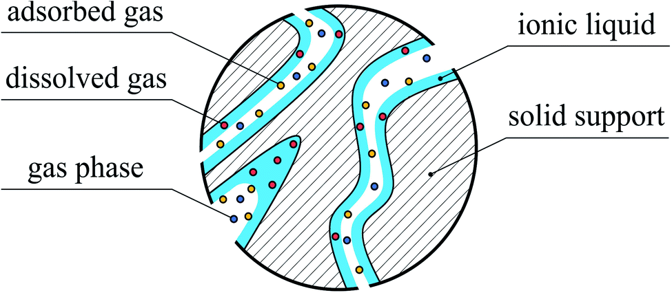 | ||
| Fig. 1 A model of the SILP with a uniform thin film of ionic liquid and partial filling of a pore exposed to the gas phase. | ||
Interaction of gases with IL films has been also explored in experimental and simulation studies. The experimental work by Roscioli and Nesbitt indicates that mechanisms of gas adsorption on and absorption in thin films of ionic liquids are very different in nature.21 For adsorption, the corrugated structure of the surface plays an important role, as evidenced from the scattering behaviour of carbon dioxide molecules interacting with the surface of ionic liquids, [BMIM]+[Tf2N]−, and [BMIM]+[BF4]−. A number of computational and experimental studies provide a more detailed view on the mechanism of gas–liquid interfacial processes. In particular, the intrinsic roughness of the ionic liquid surfaces induced by the strong electrostatic interactions between the ions22 leads to an increased surface area and thus to multiple collisions between gas molecules and the surface.21 Consequently, as gas molecules lose translational energy21 they are trapped by the strong interfacial dispersion and electrostatic (quadrupole–charge interactions) forces.8,9 This mechanism of gas–liquid interactions is responsible for rapid adsorption and formation of a dense layer of carbon dioxide on the surface of the IL as revealed by Perez-Blanco and Maginn in their computational studies.8,9 On the other hand, the solubility of gases in bulk ionic liquids is governed by other types of effects. From experimental and theoretical studies, we find a strong correlation between the solubility of CO2 and molar volume of ILs.21,23 Using molecular simulations, Klähn and Seduraman argued that the key factor influencing gas solubility is the formation of interstitial voids between the ions of the liquid that enables gas molecules to absorb in these cavities.23 What emerges from all these studies is the fact that the interaction of gases within SILP systems is governed by the processes of adsorption on the surface of the film of IL and absorption in the bulk liquid phase (Fig. 1).
A substantial body of literature has been also devoted to studying the efficiency of gas separation or gas selectivity of pure and supported ILs, where the support is provided by polymeric membranes, metal–organic frameworks (MOF), zeolites, porous silica, and carbon. Here we consider only a few typical examples of support-materials to highlight their overall influence on gas selectivity. We begin with the studies of bulk liquid systems. In a series of papers, Shiflett et al. compared experimentally obtained CO2/N2O selectivity of two ILs, [BMIM]+[BF4]−, and [BMIM]+[CH3CO2]−.24–26 Depending on the gas feed ratio, the solution of the [CH3CO2]− IL had a selectivity of 103 to 107 while the [BF4]− IL achieves selectivity of only 1.5–4.5. The 3 to 7 orders of magnitude increase in selectivity shows the significance of the choice of IL in gas separation. The strong chemical interaction between the acetate-containing ILs and CO2 increases the selectivity over N2O, the solubility of which is governed by purely physical absorption.27–29 Zeng et al. reported that gas selectivity in ILs depends on the following factors: the acid–base interactions where the anion acts as a base and CO2 as an acid; rearrangement of cations and anions upon gas absorption; formation of interstitial voids; and the strength of electrostatic and van der Waals interactions.30 For ionic liquids confined in porous structures, an interplay between interfacial and bulk behaviour of gas and liquid plays a crucial role. For instance, supported ionic liquid membranes show improved CO2/N2 and CO2/CH4 separation performance in the experiments that also depends on the nature of the anion.31,32 In particular, gas selectivity is low for [Cl]−, [BF4]− anions and high for [N(CN)2]−, [CH3CO2]− anions. Next, we consider experimental and simulation studies on MOFs impregnated with ionic liquids.33–36 These studies suggest that the presence of ILs in the pores of MOFs enhances CO2 adsorption at low pressures, whereas N2 and CH4 adsorption is unaffected. Several experimental works achieved significantly improved CO2/N2 and CO2/CH4 adsorption selectivities for a cage-type MOF (ZIF-8) tailored with [BMIM]+[Tf2N]− in comparison to the pristine ZIF-8.33,34 The authors argued that the affinity of the IL guest molecules towards CO2 as well as the pore structure of MOFs contribute towards high CO2/N2 and CO2/CH4 selectivity. In addition, the steric effects between the cage and bulky molecules of the IL reduce the effective cage size, improving the sieving properties of the composite material. In another work, Shi and Sorescu reported enhanced CO2/H2 selectivity of carbon nanotubes filled with the ionic liquid, [HMIM]+[Tf2N]−, in comparison to the performance of the pure support and pure IL.37 Using computational modelling, the authors showed that CO2 favorably interacts with the confined IL because of the strong influence from the support while the solubility of H2 remains almost the same as for the pure IL, thus explaining the higher gas selectivity. To summarize these observations, accumulated from both computer simulations and experiments, commonly used porous materials including zeolites, porous silica and carbon completely loaded with ionic liquid demonstrate an increased selectivity towards CO2.36,37
Although the majority of works recognize the importance of the relation between interfacial and bulk thermodynamic properties of SILPs, not many studies so far have considered the competition of these two contributions towards gas adsorption. From Fig. 1, we intuitively recognize the distinct regions associated with gas absorption and with gas adsorption. To explore both processes mesoporous structures (pore width 2–50 nm according to IUPAC classification) must be employed to provide enough space for the formation of ionic liquid films and gas–liquid interfaces. What are the relative contributions of these regions to the overall gas uptake and selectivity of SILPs and how do these contributions depend on the thickness of the film and interfacial structure? This is the main scientific question posed here.
To a significant extent, the current study is inspired by the work of Perez-Blanco and Maginn.8 In their molecular dynamics simulations, they constructed a thin film of the ionic liquid, [BMIM]+[Tf2N]−, and investigated the structure and interaction of this film with carbon dioxide. Here we capitalize on the recent developments in the accurate characterization of the structure of the interfacial region between two phases. The Identification of Truly Interfacial Molecules (ITIM) method, proposed by Partay et al., recognizes that the surface separating two fluid phases may have a complex structure featuring undulations, as a result of thermal fluctuations.38 In this work, we employ the ITIM for the first time to both the IL phase and the gas phase to provide an accurate picture of the structure of these two phases in contact.
Application of the ITIM analysis to the system of a thin film of an IL and a gas phase also allows us to revisit the definition of the boundary separating these two phases. In the Methodology section, we contrast this definition with well-established Gibbs and Guggenheim conventions. Building on the ITIM definition of this boundary, we explore absorption of carbon dioxide and nitrogen in the bulk region of the film and adsorption on the surface and propose an approach to quantify these contributions. We verify this approach by comparing experimentally and computationally obtained absorption isotherms for a single component gas phase, carbon dioxide. Further, we show that the overall behaviour of the film is a function of the film thickness (in addition to other parameters such as temperature, pressure and the composition of the gas). We reflect on how the gas capacity and selectivity of the film depend on its thickness and propose a model that, under certain assumptions and given the required experimental data, can estimate these properties in SILPs, which should facilitate engineering of new supported ionic liquid materials with the designed adsorptive functionalities.
2. Methodology
2.1. Molecular simulation
In the present work, we use molecular simulations to model physical gas adsorption on the surface of a film of ionic liquid. Fig. 2 shows the chemical composition and molecular structure of the ionic liquid, 1-butyl-3-methylimidazolium hexafluorophosphate, [BMIM]+[PF6]−. The molecule consists of a spherical anion, [PF6]−, and a large cation, [BMIM]+, which features the positively charged imidazolium ring with methyl and butyl chains attached to it. In the bulk ionic liquid, the anion tends to stay close to the most acidic proton, –HR, which plays a significant role in hydrogen bonding between the anion and the cation.39 Thermodynamic properties of this ionic liquid have been broadly studied in simulations and experiments providing us with ample data for comparison and validation. Details on the molecular structure and properties of bulk ionic liquids are presented in the work of Doherty et al.39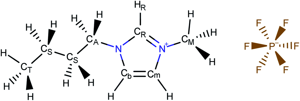 | ||
| Fig. 2 Atomistic representation of the ionic liquid, 1-butyl-3-methylimidazolium hexafluorophosphate, [BMIM]+[PF6]−. | ||
Fig. 3(a) shows the molecular visualization of the initial system containing a film of the ionic liquid exposed to the gas phase. The liquid phase consists of 500 ion pairs that constitute a film of about 5.80 nm thickness along the z-axis and a side length along the x- and y-axes equal to 5.64 nm. Such a model is computationally tractable and provides both a bulk liquid region that is thick enough to ensure reliable statistics for the amount of gas absorbed in the region, and a surface area that is sufficiently large to observe gas adsorption. The gas phase consists of either carbon dioxide or nitrogen, or their mixture as shown in Fig. 3. Adsorption properties of the film are studied at different temperatures and gas pressures by varying the size of the simulation cell along the z-axis and changing the number of gas molecules in the range from 100 to 350 for each component. The full list of simulations including the composition of the gas phase and the size of the cell is provided in Table S1 of the ESI† file.
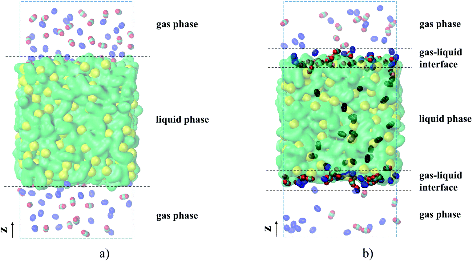 | ||
| Fig. 3 Computer visualizations of (a) a film of ionic liquid [BMIM]+[PF6]− consisting of 500 ion pairs: cations [BMIM]+ (green) and anions [PF6]− (yellow); randomly packed 100 CO2 (red) and 100 N2 (blue) gas molecules; (b) the same system after 10 ns of equilibration and 55 ns of sampling. Opaque gas molecules are adsorbed on the surface of the ionic liquid; transparent gas molecules correspond to the bulk gas phase; black gas molecules are dissolved in the bulk liquid phase. | ||
For all adsorption simulations, we use the Molecular Dynamics (MD) method implemented in the Gromacs simulation package (v.5.1.2).40 Each simulation of gas adsorption starts from the same type of initial configuration shown in Fig. 3(a), obtained using the following protocol. First, we generate a sample of a bulk ionic liquid. For this, 500 ion pairs are randomly packed in a cubic cell using Packmol software41 and equilibrated in the isothermal-isobaric ensemble for 10 ns, with a 1 fs time step. To validate our simulations, we compared key structural characteristics and thermodynamic properties (density, surface tension, and self-diffusion coefficient) of [BMIM]+[PF6]− to the reference results of Doherty et al.,39 based on the same model of the ionic liquid. These results are provided in Table S2 (ESI†) and they are in a good agreement with the available experimental and reference data. The ionic liquid pre-equilibrated at 298 K, which occupies a cubic cell with a side length of 5.64 nm, is further used to generate a system such as that shown in Fig. 3(a). In particular, we extend the size of the box along the z-axis to the required value and randomly distribute gas molecules in the void phase. In all our MD simulations, we let the initial gas–liquid interfacial systems reach equilibrium for 10 ns and then run the simulation for an additional 55 ns with 1 fs time step to collect data. The simulations of the interfacial systems are performed in the canonical ensemble at fixed temperature, volume of the system and total number of molecules of each species. We use the Peng–Robinson equation of state42 for calculating partial pressures of each gas component where gas density and volume correspond to the bulk gas region (see ESI† for a justification of this choice). A constant temperature (298, 323, 343, or 393 K) is maintained via the V-rescale thermostat, which is proved analytically to sample a canonical ensemble.43Fig. 3(b) shows a film of ionic liquid at equilibrium with the gas phase. Fully detailed parameters of the MD simulations are reported in the ESI.†
A full set of parameters describing inter- and intramolecular interactions associated with the molecular model of ionic liquid and gas molecules is also reported in the ESI.† Parameters related to the Lennard-Jones and Coulomb terms as well as to the intramolecular interaction terms (bond stretching, bending, torsional potential) correspond to the OPLS force field for the ionic liquid, [BMIM]+[PF6]−, with partial charges scaled down by 0.8, as proposed by Doherty et al.39 For CO2 we adopt the TraPPE-flex force field that accounts for all energy terms.44 Nitrogen molecules are modeled using the TraPPE force field developed by Potoff et al.45
2.2. Structure characterization tools
One of the key objectives of this work is to explore the intrinsic density profiles of the gas adsorbed on the surface of the ionic liquid film. The analysis of fluid interfaces is not trivial and is complicated by the presence of inherent thermal fluctuations or capillary waves.46,47 To illustrate this issue, consider the schematics in Fig. 4. The figure shows a part of the fluid surface, with the red particles corresponding to the bulk region and the blue particles to the interface. The surface also features undulations, typical for liquid–gas and liquid–liquid interfaces. On the left, in Fig. 4(a), we demonstrate how a standard approach to obtain the density profiles would see this system. In this approach, the system is split into uniform slabs perpendicular to the interface normal, and the atomic number density in each slab is calculated according to eqn (1):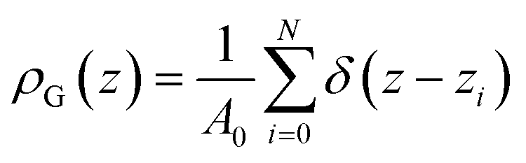 | (1) |
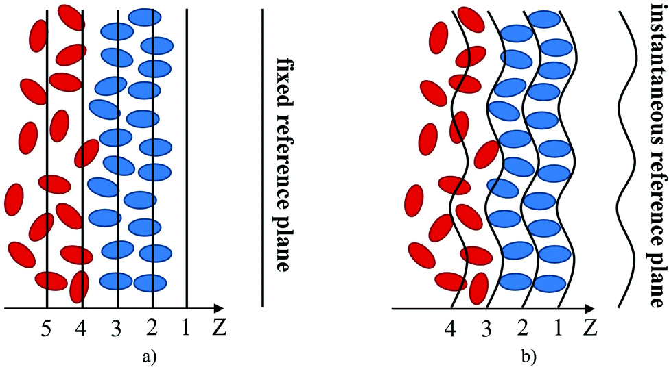 | ||
| Fig. 4 Identification of the fluid interface: (a) global analysis; (b) ITIM analysis. Black lines and curves set the boundaries of the sampling bins; red and blue ellipses represent particles (atoms, ions) of the bulk and interfacial regions of the fluid, respectively. In the ITIM analysis, the origin of a grid (plane 1) shifts towards the instantaneous position of the interface. | ||
We expect that the resulting density profiles should have bulk density values in the region of red particles gradually diminishing across the interface and, according to the schematics, reaching zero values on the right side of the diagram. This picture will be further re-enforced with actual density profiles later in the section. However, it is clear that the standard approach (we call it “global”) overlooks significant ordering and structure of fluid particles on the surface. This structure and ordering become apparent in Fig. 4(b) where, using the same fluid configuration, the corrugated slabs trace the instantaneous shape of the liquid interface. Density profiles constructed according to a system of parallel corrugated slabs should reveal the intrinsic ordering of the fluid molecules at the surface. To implement this approach, Partay et al.38 proposed a method of identification of truly interfacial molecules (ITIM), which was later extended by Jorge et al.46,47 to enable the calculation of density profiles relative to the intrinsic surface. Formally, these profiles are calculated using eqn (2) and the theoretical foundation of the method is described in detail in corresponding publications:38,46,47
 | (2) |
The ITIM analysis of all gas–liquid interfacial systems is performed according to the following methodology. The first step of the ITIM analysis is detecting the set of true interfacial atoms and of the molecules (ions) associated with them. Atoms located at the interface are identified by an algorithm, which generates a series of probe spheres moving perpendicularly to the x–y plane along a grid of test lines. Each atom in the analysis is represented by a sphere of a diameter equal to its Lennard-Jones collision diameter σ. The spacing between test lines should be fine enough to reveal the structural details of the surface. We choose this parameter equal to 0.05 nm to be consistent with the original work of Jorge et al.46 Reasonable values for the probe sphere radius are chosen to be 0.2 and 0.125 nm to probe the positions of atoms of the ionic liquid phase and the gas phase, respectively. Several studies show that these values provide optimum results for different fluid phases, including ionic liquids.38,48,49 Interfacial atoms are defined as the first atoms touched by a probe sphere. Interfacial molecules are defined as those having at least one interfacial atom.
The second step of the method is generating consecutive corrugated slabs along the normal to the x–y plane, at equal distance from each other, that match the real shape of the surface layer (black lines in Fig. 4(b)).47 The width of each slab parallel to the (x × y) plane is equal to 0.04 nm. To build a continuous intrinsic surface ξ(xi,yi) defining the surface layer at any (x, y) point, a triangular interpolation algorithm is used. This is found to be the most efficient way of accurately computing intrinsic profiles based on a finite set of interfacial atomic positions.47 Additional details regarding the ITIM analysis of the gas–liquid interfacial systems studied here are provided in the ESI.†
For illustration, Fig. 5 compares density profiles for the ionic liquid, [BMIM]+[PF6]− and gases at 298 K calculated using both the global and the ITIM analyses. Density profiles for all simulated systems are highly symmetric, which is an indication of well-equilibrated simulations, despite the relatively high viscosity of the ionic liquid phase.50 Therefore, all profiles were symmetrized relative to the ordinate axis, which goes through the center of the liquid phase. As expected, the global density of the ionic liquid presented in Fig. 5(a) slowly increases in the interfacial region resulting in a moderate maximum in comparison to constant density in the bulk region. In contrast, the intrinsic density shown in Fig. 5(b) exhibits a sharp and high peak located at the average position of the true interface, which is attributed to the interfacial atoms. The second peak is associated with atoms that are chemically bonded to the same interfacial molecules. The third peak mostly belongs to the sub-surface molecular layer. The fourth peak is fully attributed to molecules residing beneath the interface. The profile exhibits a few more oscillations that eventually decay to the value of the bulk liquid. These characteristics of the ionic liquid interface mirror those described in detail in previous studies of the same system.48,51
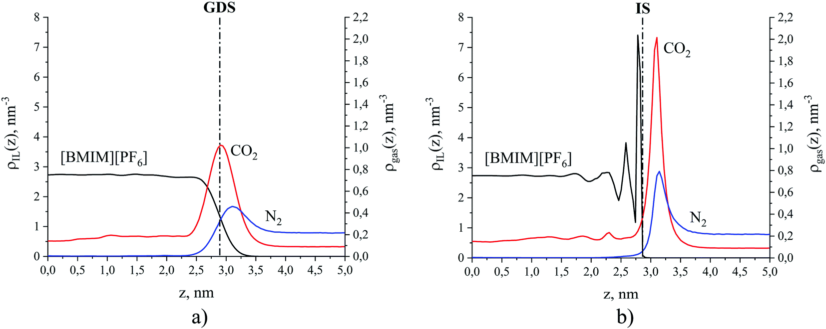 | ||
| Fig. 5 Number density profiles for [BMIM]+[PF6]− (black curve) and gases CO2 (red curve) and N2 (blue curve) at 298 K: (a) global analysis, dash-dot line is the Gibbs dividing surface (GDS); (b) ITIM analysis, dash-dot line is the ITIM surface (IS). For the purpose of illustration, the profiles here correspond to the conditions of system 12 in Table 1 of the Discussion section. | ||
The intrinsic density profiles of gases, calculated here for the first time, indicate the actual position of gas molecules on the surface of the ionic liquid and between the interfacial and sub-surface layers. The global density profiles of gases have broad peaks that overlap with the profile of the liquid phase and show a constant density of CO2 dissolved in the bulk ionic liquid. It is clear that intrinsic density profiles for the ionic liquid and gas species provide a more accurate and detailed description of the structure near the interface. Furthermore, the true position of the gas phase relative to the ITIM surface (defined in the next section) allows us to correctly calculate the excess amount adsorbed. For example, the comparison of the excess amounts calculated from the global density profile (relative to the GDS) and ITIM density profile (relative to the IS) for the case presented in Fig. 5 leads to the difference in values of 1% for CO2 and 37% for N2 (see ESI† for defining different regions of gas density profiles). Thus, we use intrinsic density profiles to determine the boundaries of the interfacial gas–liquid region and to derive properties that characterize gas adsorption and absorption in this region.
2.3. Definition of the interface
In this section, we define the location of the surface of the liquid phase and boundaries of different regions such as bulk gas, gas–liquid interface and bulk liquid. Historically, the fluid–fluid interface has been defined using Gibbs52 or Guggenheim53 conventions. According to the Gibbs treatment of the surface, the volume of the interfacial region is set to zero meaning that all surface properties are ascribed to a plane, known as the Gibbs dividing surface.54Fig. 6(a) illustrates how the excess amount adsorbed is calculated according to the Gibbs convention. Horizontal lines corresponding to the bulk densities of each phase are extrapolated to the Gibbs dividing surface at the origin of the coordinate. The red and blue areas under the solute density profiles are determined according to eqn (3).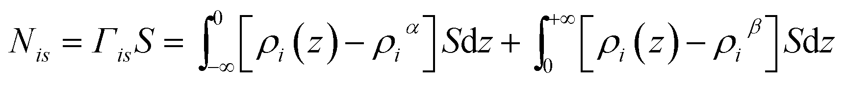 | (3) |
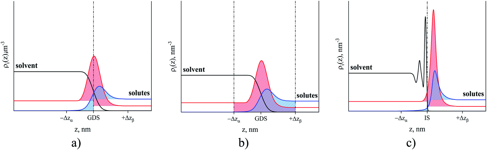 | ||
| Fig. 6 Number density profiles of hypothetical solvent (black curve) and solutes that are represented by soluble (red curve) and non-soluble components (blue curve). (a) The Gibbs convention: dash-dot line is the Gibbs dividing surface; (b) the Guggenheim convention: Δzα is the thickness of the interface into phase α or solvent, and Δzβ is the thickness of the interface into phase β or solute; (c) the ITIM convention: dash-dot line is the ITIM surface. Red and blue areas are the excess amount adsorbed according to each convention. | ||
In comparison to the Gibbs definition of the surface phase, Guggenheim introduced a finite surface-phase thickness encompassing the interfacial region. Fig. 6(b) shows the adsorbed amount (red area) in the interfacial region between –Δzα and Δzβ. These two boundaries of the interfacial region extend broadly enough that the densities of the surrounding solvent and solute phases are uniform, corresponding to bulk densities. Eqn (4) demonstrates how the amount of solute adsorbed on the surface is calculated using the Guggenheim definition of the surface phase.
 | (4) |
Another definition of the boundary between the two phases naturally originates from the ITIM analysis. Indeed, the gas phase concentration of the IL is essentially zero (due to low volatility) and the sharp first peak in the density of the IL provides a natural way to divide the system into the ionic liquid region on the left of the dash-dot line in Fig. 6(c) and the gas region on the right of that line. Moreover, the ITIM boundary allows us to make another connection to the properties measured experimentally. As has been mentioned, we are interested in developing a predictive model of gas adsorption in SILP systems. In the current study, we assume that the IL is distributed in these structures as a uniform film of a particular thickness (in a concurrent research thread we are proposing analysis to test this assumption). The surface area of a porous material, including the supported IL system, is measured in argon or nitrogen sorption experiments with BET analysis. In studies of porous materials, the computational analog of the BET surface area is the area formed by the probe molecule (argon or nitrogen) on the surface of the material.55 The surface formed by the tip of the probe molecule is often called the Connolly surface. Fig. 7(a) and (b) illustrate the similarities between the Connolly surface, accessible surface, and the ITIM surface. Hence, we argue here that the ITIM boundary and the corresponding surface (Fig. 7(c)) are closely related to the surface seen by the nitrogen or argon probe in sorption experiments (in the schematics, it corresponds to the accessible surface), allowing us to incorporate this experimental information in the construction of the predictive models as will be discussed below.
 | ||
| Fig. 7 The methodology of defining the interfacial region: (a) the Connolly convention: the solid curve is the Connolly surface, the long-dashed curve is the accessible surface; (b) the ITIM method: the solid broken line is the calculated ITIM surface. Blue circles are the particles of the solvent phase, grey circles are the probe spheres, dashed lines are the distance between the centers of particles and probe spheres, dash-dot lines are the test lines. The lower part of panel (b) shows how the surface is defined if the spacing between test lines is reduced. (c) Molecular visualization of ionic liquid, [BMIM]+[PF6]−: red volume is the bulk liquid phase, the blue area is the intrinsic surface. | ||
3. Results and discussion
3.1. Adsorption and absorption in thin films at 298 K
We begin this section by exploring the behavior of carbon dioxide and nitrogen in the vicinity of the gas–liquid interface. Binary and ternary mixtures consisting of ionic liquid with different amounts of gas (where the gas is represented by a single component of either carbon dioxide or nitrogen or their mixture) are considered at the temperature of 298 K. Table 1 summarizes all investigated systems including compositions and total pressures of the gas phase at equilibrium.| # | Composition of the gas phase, xCO2 | Total gas pressure, P, MPa |
|---|---|---|
| Binary mixtures of ionic liquid and carbon dioxide | ||
| 1 | 1.000 | 0.0925 |
| 2 | 1.000 | 0.229 |
| 3 | 1.000 | 0.350 |
| 4 | 1.000 | 0.510 |
| 5 | 1.000 | 0.632 |
| 6 | 1.000 | 0.889 |
![[thin space (1/6-em)]](https://www.rsc.org/images/entities/char_2009.gif) |
||
| Binary mixtures of ionic liquid and nitrogen | ||
| 7 | 0.000 | 0.110 |
| 8 | 0.000 | 0.373 |
| 9 | 0.000 | 0.869 |
|
||
| Ternary mixtures of ionic liquid, carbon dioxide, and nitrogen | ||
| 10 | 0.439 | 0.196 |
| 11 | 0.371 | 0.599 |
| 12 | 0.291 | 1.242 |
| 13 | 0.357 | 1.451 |
| 14 | 0.358 | 1.818 |
| 15 | 0.356 | 2.538 |
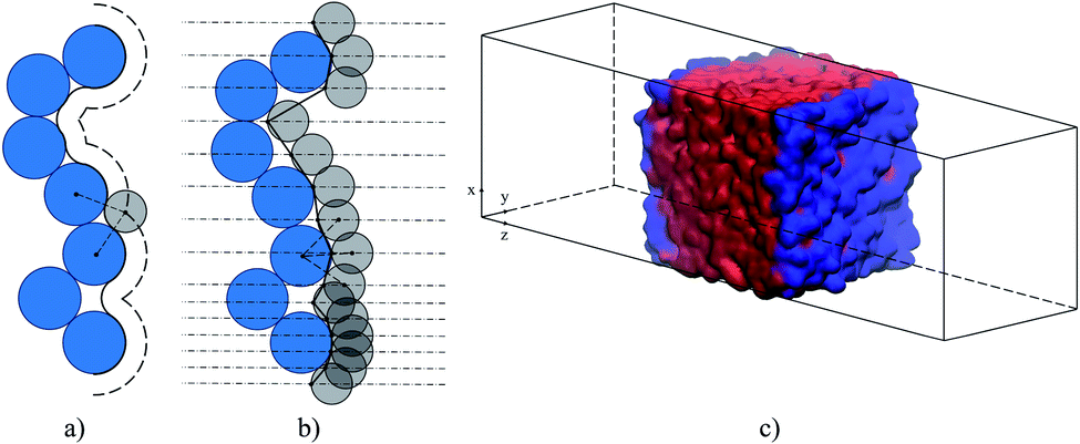
Fig. 8 provides intrinsic density profiles for carbon dioxide (a) and nitrogen (b) in these systems. From this figure, the surface of the ionic liquid (dash-dot line) acts as an attractive surface where CO2 and N2 form a dense layer. The pronounced narrow peaks corresponding to CO2 adsorption in comparison to broad peaks for N2 are a simple manifestation of the strong CO2 – interface interaction. Interestingly, CO2 molecules also accumulate between the surface and the subsurface layers of the ionic liquid (Fig. 8(a), inset). In several computational and experimental studies,48,51,56–61 authors observed mutual nanoscale self-assembly of interfacial cations and anions of ionic liquids extending up to two molecular layers that we believe may cause this gas behaviour (in a concurrent research thread we are investigating this phenomenon in detail).
 | ||
| Fig. 8 Number density profiles for (a) CO2 and (b) N2 at 298 K obtained from MD simulations of binary (dots) and ternary mixtures (solid lines) of ionic liquid and gas, where the gas consists of a mixture of carbon dioxide and nitrogen or a single component of either carbon dioxide or nitrogen. The color gradient of the lines and dots from light to dark red and grey, respectively, corresponds to an increase of partial pressure for CO2 and N2 for systems listed in Table 1. The dash line is the ITIM surface. The insets show a more detailed picture within the yellow-shaded areas. | ||
The density profiles in Fig. 8 represent the interplay between two processes. The first process is associated with gas adsorption on the surface of the film as a result of interactions between interfacial molecules of the ionic liquid and the molecules of the gas phase. The second process is the process of absorption of gas molecules into the interior of the liquid film, governed by solubility effects. Here, we focus on the quantitative assessment of the relative contribution of these processes towards the total loading of the gas, and on the understanding of conditions under which one of them dominates. Below we show that this analysis offers a route for the construction of a predictive model of adsorption of carbon dioxide and nitrogen in SILPs under certain assumptions and given a few basic parameters of the porous material such as surface area, free pore volume and the amount of the ionic liquid deposited in pores.
We are interested in defining the absolute amount adsorbed. Myers and Monson emphasize that the framework of absolute adsorption provides a rigorous and consistent approach to calculating thermodynamic properties of the system at low and high pressures.62
First, we parse the absolute amount of gas present in the system into various contributions. The definition of the ITIM surface allows us to split the system into three distinguishable parts shown in Fig. 9. The bulk gas density profile extended to the ITIM surface reflects the bulk gas contribution, shown as the blue region. Gas dissolved in the ionic liquid is shown as the red region, also extended to the ITIM surface. The remaining quantity of gas, shown as the yellow area, is defined as the excess amount adsorbed. The absolute amount of the gas in the system can be expressed therefore as:
| N = Nρ + Nσ + Nγ | (5) |
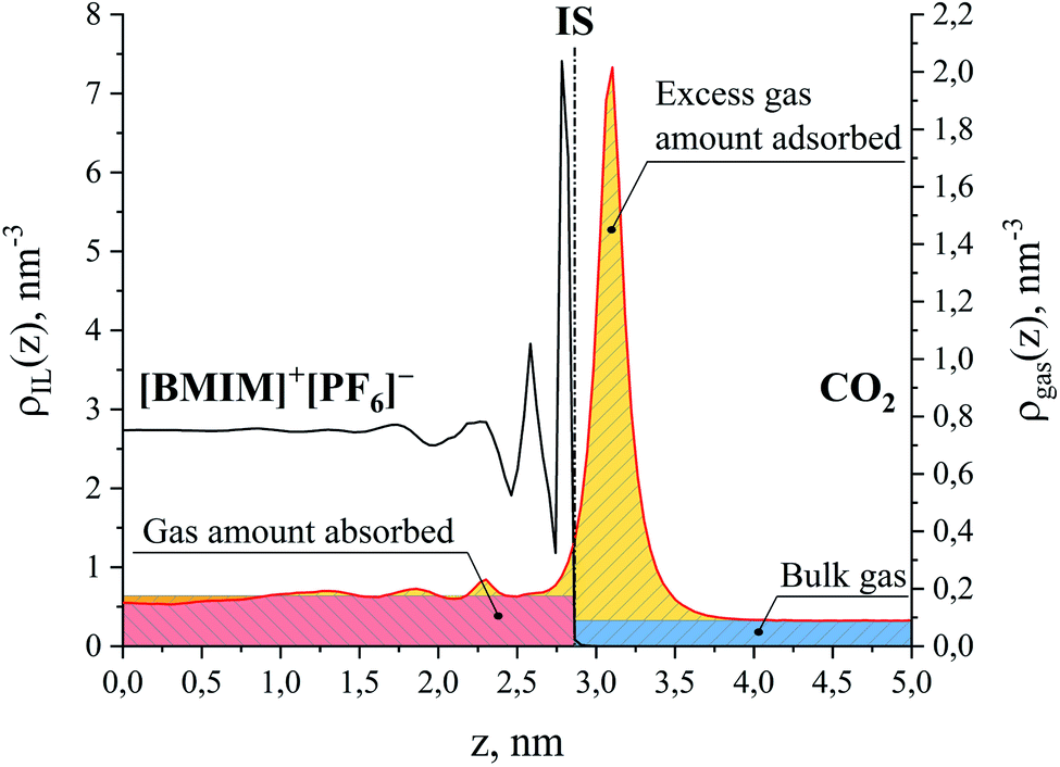 | ||
| Fig. 9 Number density profiles for ionic liquid, [BMIM]+[PF6]− (black curve) and CO2 (red curve) at 298 K. Different colors show the areas corresponding to the amount of gas absorbed in the bulk liquid phase (red), the excess amount of gas adsorbed on the surface of the liquid phase (yellow) and the amount of the bulk gas phase (blue); IS is the ITIM surface. The red region above the CO2 density profile in the ionic liquid phase overlaps with the yellow region related to the negative excess amount. For the purpose of illustration, the profiles here correspond to the conditions of system 12 in Table 1. | ||
The question we want to address now is how to estimate these three quantities, as this is what we need in order to assess the relative contributions of adsorption and absorption in the films. Prior to this, it is first important to establish whether the films under consideration are thick enough to exhibit bulk-like properties in the region away from the interface. Investigating Fig. 9, we see that, starting from the ITIM surface, the interfacial structuring of the IL (black line) gradually disappears over 1.3 nm thickness approaching the bulk density of the IL. The bulk density of the ionic liquid decreases upon gas absorption from 1315 kg m−3 for the pure IL to 1264 kg m−3 for the system containing CO2 and N2 at the total gas pressure 2.538 MPa (Table 1, sample 15). We also observe some patterns in the ordering of the dissolved CO2 molecules over the same region, with the profile (Fig. 9, red line) then becoming featureless near the middle of the IL slab. This suggests to us that the core of the film behaves like the bulk ionic liquid. Our observations are in agreement with previous research showing that structural properties of molecular liquids, including ILs, are only affected up to a few molecular layers beyond the interface.48,51,56–61 We emphasize here, however, that the current analysis does not consider possible structuring effects from the support material on the ionic liquid film. Next, we calculate the amount of gas dissolved in the bulk region of the ionic liquid film. These calculations are more challenging than could be expected because the finite size of the simulations, coupled with high viscosity, and hence long relaxation time, of the ionic liquid, lead to non-negligible statistical fluctuations in the density of the gas absorbed in the bulk volume of the film. To circumvent these difficulties, we developed an algorithm that progressively averages the gas density starting from the center of the film and moving towards the interface, until it reaches the onset of the main peak of the gas density profile, defined according to the geometric criteria explained in the ESI.† From this, we determine the constant gas density profile in the bulk liquid on the left of the ITIM surface (red region). This technique allows us to effectively take into consideration statistical fluctuations of the gas concentration near the center of the liquid slab. Fig. 10(a) summarizes the calculated CO2 solubility in the bulk region of ionic liquid films at different pressures and compares it to the experimentally measured values provided by Anthony et al.63 We observe a very good agreement between gas solubility obtained from simulations and experiments, further confirming that the bulk region of the simulated film of the ionic liquid behaves as real bulk liquid and is not affected by the presence of the interface.
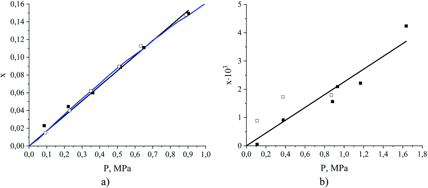 | ||
| Fig. 10 Absorption isotherms (mole fraction x as a function of partial pressure) for (a) CO2 and (b) N2 dissolved in the ionic liquid, [BMIM]+[PF6]−, at 298 K. Data points were obtained from MD simulations of binary (open symbols) and ternary (filled symbols) mixtures of ionic liquid and gas, where the gas consists of a mixture of carbon dioxide and nitrogen or a single component of either carbon dioxide or nitrogen. The blue curve is the experimental data reproduced from Anthony et al.,63 the black lines are the Henry's law models fitted to the simulation data for ternary mixtures. | ||
Fig. 10(b) shows an isotherm of nitrogen absorption in the bulk region of the ionic liquid film at 298 K. We observe very low solubility of nitrogen, which exacerbates statistical uncertainties and causes broad scattering of the data points. Several studies confirm the low solubility of nitrogen in ionic liquids, however, the reported Henry's constants are scarce and not consistent. For instance, Henry's constant for N2 in [BMIM]+[PF6]− at 298 K is 119.2 MPa (extrapolated) as reported by Jacquemin et al.64 and >2000 MPa as reported by Anthony et al.63 at the same temperature by measuring the single component experimental isotherms. In all further calculations, we use Henry's constant corresponding to the slope of the line fitted to the simulation data points (435 MPa).
Once the average gas concentrations in the bulk gas and liquid phases are determined, we can obtain the excess amount adsorbed from the integration of the density profile (Fig. 9, yellow region). Fig. 11 compares the excess amount adsorbed in simulations of binary and ternary systems. We note that the presence of the second gas component does not seem to have any significant impact on the adsorption of CO2 or N2 in the range of pressures under consideration. This is consistent with gas absorption shown in Fig. 10. Therefore, to make the presentation more compact and consistent, we predominantly focus on ternary systems while binary systems are considered for selected cases only. From Fig. 11, CO2 adsorption on the surface can be described by Henry's law in the partial pressure range up to 1 MPa, while N2 adsorption can be described by the Langmuir model.65 The fitted Langmuir model (single-component) provides a saturation capacity for N2 equal to 0.543 molecules per nm2 of the surface area and a Henry's constant equal to 3.9 ± 0.3 MPa nm2 in the low coverage regime at 298 K. The shapes of the isotherms in Fig. 11 clearly indicate different adsorption processes for the two species. This is related to the relative strength of interaction between the gases and the surface of the ionic liquid. Nitrogen is attracted by the surface, however, once the initial layer is formed, the interaction with the next layer is much weaker, leading to the signs of saturation in the adsorption isotherm. Carbon dioxide, being slightly subcritical under conditions of interest, interacts strongly with the surface and with the already adsorbed molecules of carbon dioxide, leading to a continuous increase of the amount adsorbed on the surface as shown in Fig. 11(a).
 | ||
| Fig. 11 Excess amount of gas adsorbed per unit of the surface area of ionic liquid film for (a) CO2 and (b) N2 at 298 K obtained from MD simulations of binary (open symbols) and ternary mixtures (filled symbols) of ionic liquid and gas, where the gas consists of a mixture of carbon dioxide and nitrogen or a single component of either carbon dioxide or nitrogen. The black lines are the Henry's law models for carbon dioxide and nitrogen; the red curve is the Langmuir model for nitrogen (single-site, single-component) fitted to the simulation data for ternary mixtures. | ||
Having investigated adsorption on the surface and absorption in the bulk liquid we explore the competition between the surface and bulk properties of the film. Fig. 12 illustrates the possible scenarios of this competition. As the thickness of the ionic liquid film decreases, the interfacial properties dominate. This would be the case for supported liquid phase materials where the ionic liquid is uniformly distributed as a thin film on the surface of pores (Fig. 12(a)). At some thickness of the film (Fig. 12(b)), the amount of gas dissolved in the bulk volume is equal to the amount adsorbed on the surface. We denote the thickness of the film corresponding to this situation as the equipartition thickness, heq. It is a quantitative metric that evaluates the prevalence of surface adsorption or bulk absorption properties of ionic liquid films. Finally, the bulk properties of ionic liquid will dominate the overall behavior if the film is very thick or the pores of the material are completely filled with the liquid phase as illustrated in Fig. 12(c).
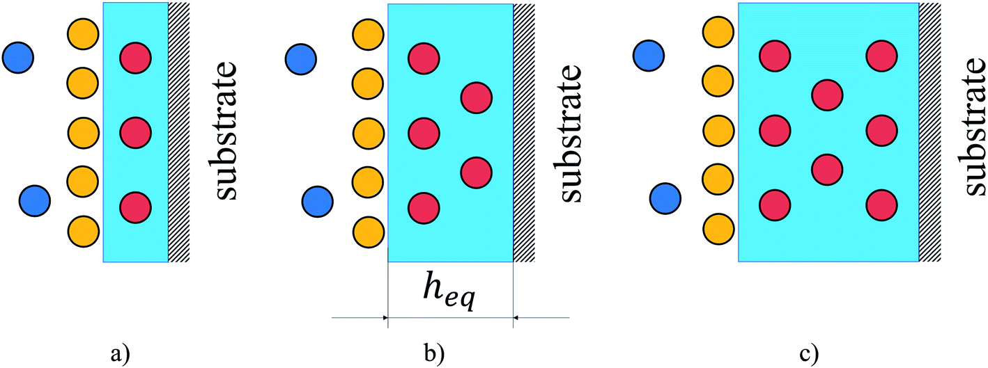 | ||
| Fig. 12 Illustration of gas adsorption on the surface of a film of ionic liquid in comparison to gas absorption in the bulk liquid volume for different film thicknesses: (a) surface properties dominate; (b) surface and bulk properties have comparable gas capacity; (c) bulk properties dominate. Circles are gas molecules where dark blue represents the bulk gas phase, yellow is the excess adsorbed on the surface and red is the amount absorbed in the liquid phase (light blue region); heq is the equipartition thickness, nm. Color-coding matches that in Fig. 1 and 9. | ||
Mathematically, the balance between the bulk absorption and surface adsorption contributions encoded in the equipartition thickness can be expressed as:
| Nρ = Nσ | (6) |
The amount absorbed in the film can be obtained as 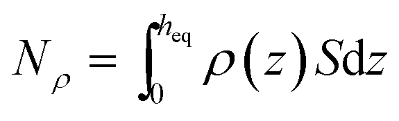 , where ρ is the number density of gas in the bulk volume of ionic liquid, nm−3, S is the surface area, nm2. If the absorbed density is uniform or represents the average value of gas solubility in the liquid phase, this expression simplifies to Nρ = ρSheq. The excess amount is obtained via Nσ = Sσ, where σ is the excess number density of gas on surface of ionic liquid, nm−2. Because densities of gas adsorbed at the interface and dissolved in the liquid phase depend on pressure, the equipartition thickness is a function of pressure as well. Given the condition eqn (6) above and after the cancellation of terms, we obtain:
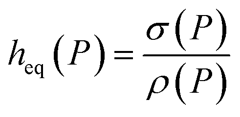 | (7) |
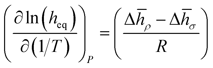
Eqn (7) shows that if gas is not soluble in the liquid phase, heq approaches infinity. This means that heq should be much larger for nitrogen in comparison to carbon dioxide. Thus, the equipartition thickness directly depends on the chemical nature of the IL and the gas. Moreover, at infinitely low gas solubility and adsorption on the surface, the equipartition thickness becomes independent of pressure. In the ESI,† we derive eqn (8) that shows the relation between the equipartition thickness and Henry's constants. Since Henry's constant depends only on temperature, this equation also provides a direct relation between the equipartition thickness and temperature, which is considered below.
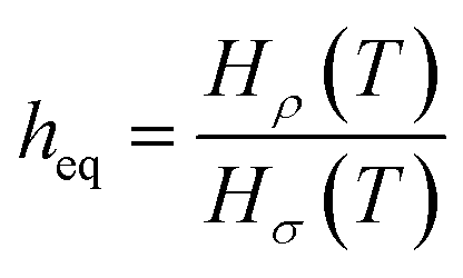 | (8) |
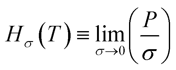 , MPa nm2, Hρ is Henry's constant of gas absorption in the bulk liquid phase defined as
 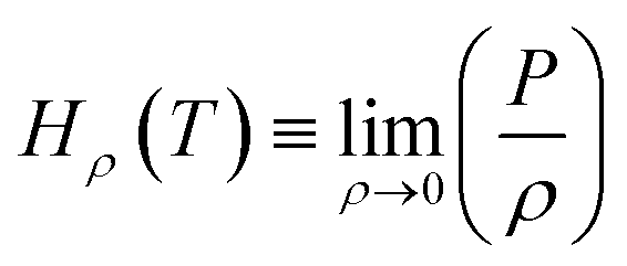 , MPa nm3. In the definitions of the Henry's constants, weak dependence on pressure and ideal gas phase are assumed.
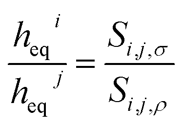
We can anticipate that depending on the nature of the fluid–fluid interactions there will be several possible functional forms of the equipartition thickness versus pressure. As eqn (8) shows, the equipartition thickness is a constant value for adsorption and absorption of a gas obeying Henry's law. At high pressures, a divergence from Henry's law is observed for solubilities in the liquid phase and for adsorption at the interface, leading to consequent changes in the equipartition thickness. To investigate this, we now consider the equipartition thickness calculated according to eqn (7) and (8) as a function of the partial pressure of carbon dioxide and nitrogen. Fig. 13 shows individual simulated results (dots). For carbon dioxide (Fig. 13(a)), we also plot a black line representing the result based on the ratio of the two Henry's constants (eqn (8)), one from the slope of the fitted line in Fig. 10(a), and one based on the slope of the line in Fig. 11(a). For nitrogen, in Fig. 13(b), the red curve corresponds to eqn (7), with ρ(P) provided Henry's law approximation in Fig. 10(b) and σ(P) obtained from the Langmuir fit in Fig. 11(b). For carbon dioxide, the equipartition thickness is independent of pressure and is equal to 2.5 nm calculated according to eqn (8). An increase in partial pressure leads to higher CO2 adsorption at the gas–liquid interface and to a proportional increase in the amount of CO2 dissolved in the bulk volume of the liquid phase (Fig. 10(a) and 11(a)). Due to the low solubility of nitrogen in the ionic liquid, we observe broad scattering in Fig. 10(b) which leads to scattered data in Fig. 13(b). Using eqn (7) we see that the equipartition thickness is not a constant value but decreases as a function of pressure (red curve) due to deviations from Henry's law for N2 adsorption (Fig. 11(b)), and is equal to 41 nm at infinitely low pressure (black circle at P = 0 MPa). The main outcome of the analysis presented in Fig. 13(a) for carbon dioxide, is that at a given temperature the equipartition thickness is not a function of gas composition or pressure in the low-pressure region. As we will demonstrate below, this behavior can be exploited in predicting the absolute amount adsorbed.
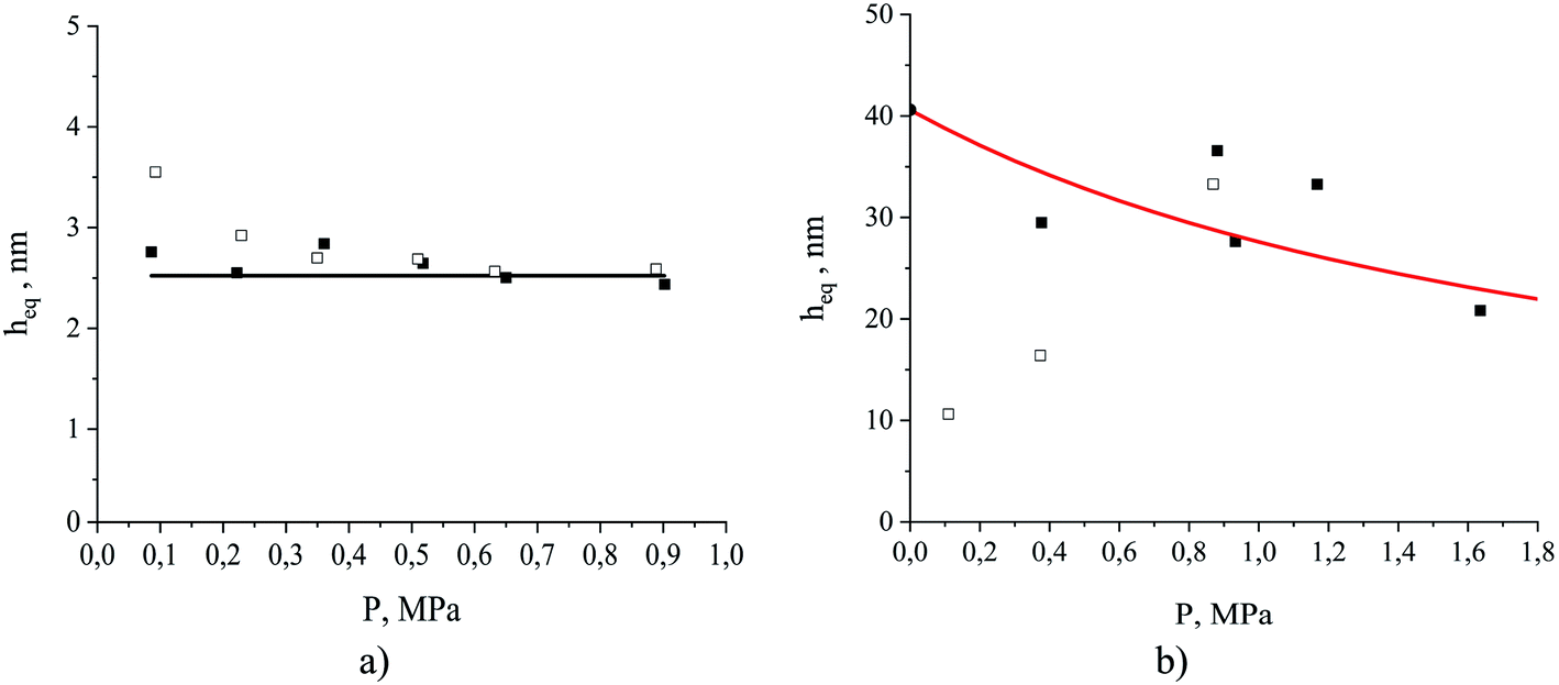 | ||
| Fig. 13 The equipartition thickness as a function of partial pressure for (a) CO2 and (b) N2 at 298 K. The simulated system contains ionic liquid, [BMIM]+[PF6]−, exposed to the corresponding single gas component (open square symbols) or a mixture of CO2 and N2 (filled square symbols); the black line and the black filled circle at P = 0 MPa for (b) are the values calculated according to eqn (8); the red curve is calculated according to eqn (7) using the Langmuir model for N2 adsorption and Henry's law model for N2 absorption. | ||
We now turn our attention to the gas selectivity of the film of the ionic liquid. For a film of ionic liquid, gas selectivities of the bulk liquid and the interfacial region both contribute to the total selectivity. Since, in the low-pressure limit, selectivity is the relation between the Henry's constants of two gases (in our case, CO2 and N2), we, using eqn (8), can derive the relation (9) between gas selectivities and equipartition thicknesses (full derivations of this and subsequent equations are provided in the ESI†):
 | (9) |
 , where subscript γ reflects properties in the bulk gas phase.
Eqn (9) provides an important link between the experimentally measurable bulk selectivity and the interfacial selectivity which is not directly available from the experiments. While eqn (9) considers the interface and the bulk liquid as two separate sub-systems of the film, what is also important to address is how the presence of the gas–liquid interface changes the overall selectivity of a whole film as a function of its thickness. Eqn (10) calculates the selectivity of CO2 with respect to N2 taking into account the influence of the interface:
 | (10) |
While eqn (10) is valid for any pressure range, it can be transformed into eqn (11) which now calculates the ideal selectivity of the film as a function of its thickness.
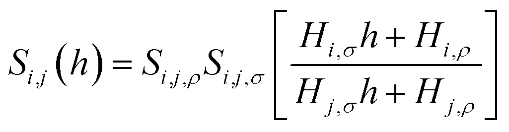 | (11) |
In Fig. 14, we consider the behavior of the CO2/N2 selectivity as a function of film thickness for two special scenarios. The first scenario corresponds to a situation where absorption and adsorption processes obey Henry's law regime for both gases, and hence eqn (11) applies to calculate selectivity, which we denote as SH. In the second scenario, we consider the capture of carbon dioxide from flue gas, with a composition corresponding to 15% of carbon dioxide, 85% of nitrogen and a total pressure equal to 1 atm. This selectivity, denoted as SFG, is calculated according to eqn (10) where we use the Peng–Robinson equation of state to determine Nγ, the Langmuir model to calculate NN2,σ, and fitted Henry's law models for the other three terms (Fig. 10 and 11). As we change the thickness of the film, at fixed temperature and partial pressure conditions, the relative contributions of surface- and liquid-related terms in eqn (10) and (11) change, thus affecting the selectivity. According to the analysis above, the amount of gas adsorbed, Nσ, on the ITIM surface of zero volume is independent of the thickness of the film. However, we assume that the amount of gas dissolved, Nρ, is proportional to the thickness of the film and corresponds to gas solubility of the bulk IL. As the thickness of the film approaches a monolayer thickness of roughly 0.8 nm, the amount absorbed in the bulk region, Nρ, is zero (the system does not have a bulk region), thus, the system is governed by the surface properties only, leading to low total selectivity of 5.2 (Fig. 14). As the total gas pressure increases, the total selectivity also increases as deduced from eqn (10). On the other hand, if the thickness of the film approaches infinity or the surface area is negligible (Fig. 12(c)), the total selectivity of the film approaches the bulk selectivity of 83. Interestingly, the presence of the interface significantly changes gas selectivity depending on the regime of adsorption. For instance, in the case of Henry's law regime for solubility and adsorption (Fig. 14, black curve), the presence of the interface drastically lowers gas selectivity, SH, for films of any reasonably practical thickness (Fig. 14(b)). In contrast, considering adsorption and absorption from the flue gas when adsorption of nitrogen does not obey Henry's law anymore, the gas selectivity quickly changes as the film gets thicker and reaches 58 at the equipartition thickness of 2.5 nm with respect to CO2. From Fig. 14, we conclude that independently of the regime, the presence of ionic liquid inside a porous material sacrifices selectivity in favor of adsorption capacity, relative to the bulk ionic liquid.
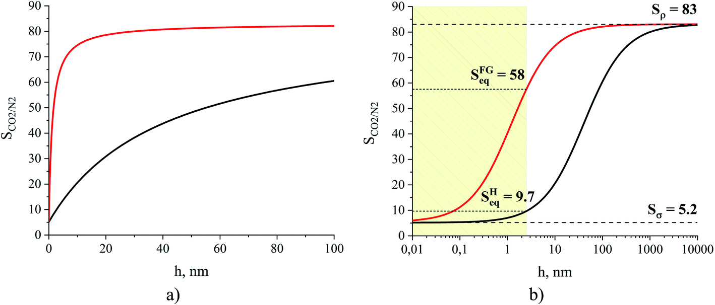 | ||
| Fig. 14 Gas CO2/N2 selectivity of an ionic liquid film, [BMIM]+[PF6]−, at 298 K presented on linear (a) and logarithmic (b) scales for the x-axis. The black curve represents the change of the ideal selectivity, SH, calculated from eqn (11), while the red curve is the change of selectivity, SFG, for a hypothetical system consisting of the film of the ionic liquid and the flue gas containing 15% of CO2 and 85% of N2 at a total pressure equal to 1 atm, calculated from eqn (10); Sρ is the gas selectivity of the bulk ionic liquid, Sσ is the interfacial gas selectivity, Seq is the gas selectivity for a film of the equipartition thickness with respect to CO2. | ||
3.2. Temperature dependence of competitive adsorption and absorption properties of thin films
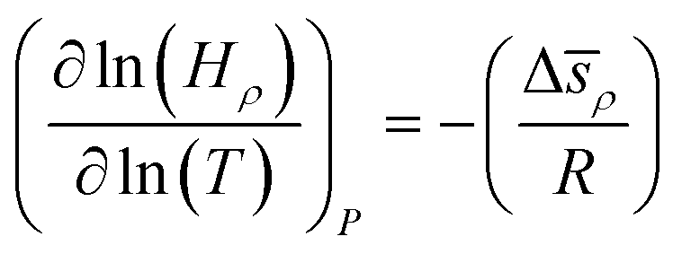
How does the balance between adsorptive and absorptive properties of the film depend on temperature? What is the impact of temperature on the overall selectivity of the film? These are the main questions we seek to address in this section. To begin with, it is instructive to briefly review what is currently known about solubility of gases in ionic liquids as a function of temperature. Within classical thermodynamics, the following relations describe how the Henry's constant of absorption depends on temperature: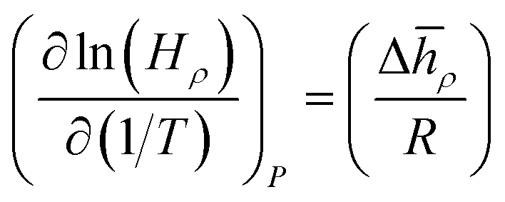 | (12) |
 | (13) |
![[h with combining macron]](https://www.rsc.org/images/entities/i_char_0068_0304.gif) ρ = ρ − γ, J mol−1, and Δ
ρ = ρ − γ, J mol−1, and Δ![[s with combining macron]](https://www.rsc.org/images/entities/i_char_0073_0304.gif) ρ = ρ − γ, J mol−1 K−1, are the partial molar change of enthalpy and entropy of absorption, respectively. In these expressions, ρ, γ are partial molar enthalpies of the solute in the liquid phase (ρ) and in the gas phase (γ); and ρ and γ are the corresponding partial molar entropies; R is the universal gas constant and all other terms are defined as before. For solutes below the critical point, Δ is negative, the process of dissolving is exothermic, and therefore solubility decreases with temperature (the Henry's constant increases with temperature). Similarly, from eqn (13), if the partial molar entropy change is negative, the Henry's constant increases with temperature and solubility decreases with temperature. However, for gases that have very low solubility (i.e. gases far away from the critical point), Δ is positive and solubility increases with temperature. Detailed consideration of these effects is provided in Sandler66 and Prausnitz et al.67
ρ = ρ − γ, J mol−1 K−1, are the partial molar change of enthalpy and entropy of absorption, respectively. In these expressions, ρ, γ are partial molar enthalpies of the solute in the liquid phase (ρ) and in the gas phase (γ); and ρ and γ are the corresponding partial molar entropies; R is the universal gas constant and all other terms are defined as before. For solutes below the critical point, Δ is negative, the process of dissolving is exothermic, and therefore solubility decreases with temperature (the Henry's constant increases with temperature). Similarly, from eqn (13), if the partial molar entropy change is negative, the Henry's constant increases with temperature and solubility decreases with temperature. However, for gases that have very low solubility (i.e. gases far away from the critical point), Δ is positive and solubility increases with temperature. Detailed consideration of these effects is provided in Sandler66 and Prausnitz et al.67
We now turn our attention to the behavior of the system under consideration at elevated temperatures (323, 343 and 393 K). The composition and corresponding equilibrium gas pressure of the studied systems are listed in Table S1.†
The approach proposed in this study allows us to decouple and explore individually absorption and adsorption effects in the ionic liquid film. Individual absorption and excess adsorption isotherms are presented in Fig. S2 of the ESI.† According to this figure, solubility of carbon dioxide decreases with temperature whereas solubility of nitrogen increases with temperature. Adsorption on the surface, being an exothermic process, diminishes with temperature for both carbon dioxide and nitrogen. Let us for now adopt the Gibbsian view of the interfacial region as an infinitesimally thin surface with the excess amount associated with this surface. Thermodynamic equilibrium between the gas phase (γ) and the surface (σ) implies μi,γ = μi,σ. This relationship can be used as a starting point to derive equations similar to eqn (12) and (13): in this case, partial molar changes in enthalpy and entropy are Δσ = σ − γ and Δσ = σ − γ. Indeed, using the data at different temperatures presented in Fig. S2† and applying eqn (12) and (13), we estimate Δρ, Δρ, Δσ, Δσ. In the case of nitrogen adsorption isotherms that start to deviate from the linear regime at higher pressures, we use the initial slope of the isotherms, where the Henry's regime applies. The results are presented in Table 2.
| Gas | Absorption | Adsorption | Transition | |||
|---|---|---|---|---|---|---|
| Δρ, kJ mol−1 |
Δρ, J mol−1 K−1 |
Δσ, kJ mol−1 |
Δσ, J mol−1 K−1 |
Δρ − σ, kJ mol−1 |
Δσ − ρ, J mol−1 K−1 |
|
| CO2 | −16.1 ± 2.263 |
−53.2 ± 6.963 |
— | — | — | — |
| CO2 | −11.9 ± 0.2 | −34.7 ± 1.2 | −14.0 ± 0.3 | −40.7 ± 1.7 | 2.1 ± 0.1 | −6.0 ± 0.5 |
| N2 | 6.9 ± 0.6 | 20.1 ± 2.5 | −10.3 ± 2.4 | −29.9 ± 9.0 | 17.2 ± 1.8 | −50.0 ± 6.5 |
Table 2 also provides values of Δρ, Δρ properties available from experiments.63 The results in Table 2 can be summarized as follows. As expected, Δρ, Δρ are negative for carbon dioxide, and positive for nitrogen, consistent with the observed increasing solubility of nitrogen with temperature. The values of Δρ, Δρ for carbon dioxide are lower compared to the experimental results, but overall are reasonable. Contrary to the bulk solubility effects, adsorption of nitrogen on the surface is governed by interactions of comparable strength to that of carbon dioxide, Δσ, Δσ are negative for both gases, the process is exothermic, and the amount adsorbed diminishes with temperature at the same pressure of the gas component. Table 2 also reports the transition properties Δρ − Δσ = Δρ − σ and Δσ − Δρ = σ − ρ, reflecting the thermodynamic equilibria between the bulk liquid and surface properties. The significance of these properties will become apparent later in the section. The data above is indicative of the molecular interactions involved in the process. In particular, enthalpy of dissolution is comparable in value to the enthalpy of adsorption for carbon dioxide and values of these properties are comparable to the latent heat of evaporation for carbon dioxide, equal to 16.7 kJ mol−1 at 288 K.68 This suggests that CO2 – IL, CO2 – surface, and CO2 – CO2 interactions in the liquid state are comparable to each other in strength. The latent heat of nitrogen evaporation is ∼6 kJ mol−1.68 From Table 2, nitrogen has a stronger interaction with the surface than with its own molecules, which can be used to explain the Langmuir-type behaviour of nitrogen adsorption isotherms: once the initial layer is formed, further adsorption on the surface is governed by weaker interactions (unlike in the case of carbon dioxide where adsorbed carbon dioxide molecules serve as adsorbing sites of strength more or less equal to that of the surface itself). We note that the experimental values for latent heats of nitrogen and carbon dioxide can be directly used in the analysis of relative strengths of interaction in the molecular models employed here, since Potoff and Siepmann demonstrated the accuracy of TraPPE models in capturing these properties.45
Let us now provide an additional reflection on the increasing solubility of nitrogen with temperature in the context of the available experimental data. Data on the solubility of nitrogen in ionic liquids is scarce.69 Therefore, we analyze the same review-paper for additional data on the solubility of argon in ionic liquids at ambient conditions. Argon has a critical temperature similar to nitrogen (150.7 K for argon and 126.2 K for nitrogen68) and therefore its solubility behavior should be similar to nitrogen. For comparison, the critical point of carbon dioxide is 304.1 K.68 We also consider [BMIM]+[BF4]− because it exhibits structural and gas solvation properties similar to those of [BMIM]+[PF6]−.23 Anthony et al.63 reported an increase in experimentally measured argon solubility in [BMIM]+[PF6]− as a function of increasing temperature from 283 to 323 K, while Jacquemin et al.64 showed a decrease in argon solubility in the same solvent and temperature range. For the same ionic liquid, Finotello et al. observed an increasing solubility trend of nitrogen as the temperature increases.70 From these studies, it seems that the picture is not fully conclusive and further investigation is required on the solubility of gases in ILs. This is also echoed by the data available for other gases and systems. For instance, some research groups observe decreased solubility experimentally measured and computationally calculated for sparingly soluble species such as oxygen and hydrogen in ILs at elevated temperatures,63,71–73 while other groups observe an increase in the solubility.64,74
We now can return to the original question posed in this section and address how properties reflecting the balance between absorptive and adsorptive characteristics of the film change with temperature. In the ESI† we demonstrate that in the Henry's law regime there is a simple dependence of the equipartition thickness on the thermodynamic properties introduced in Table 2:
 | (14) |
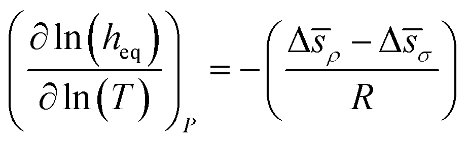 | (15) |
Using these formulae and assuming weak temperature dependence of the terms on the right, we obtain the results presented in Fig. 15.
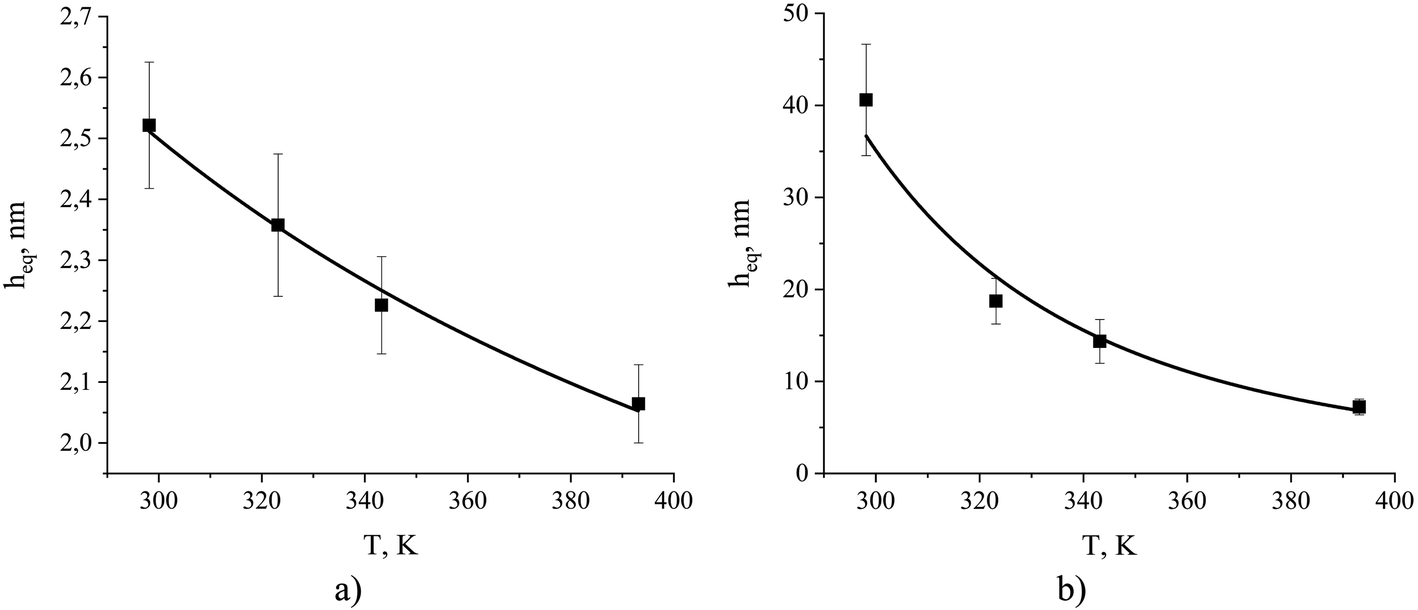 | ||
| Fig. 15 The equipartition thickness for (a) CO2 adsorption and (b) N2 adsorption as a function of temperature calculated according to eqn (8). The black curves are obtained from eqn (14). The simulated system contains ionic liquid, [BMIM]+[PF6]−, exposed to a mixture of CO2 and N2. Individual values of the equipartition thickness as a function of pressure are shown in Fig. S4.† | ||
According to Fig. 15, the observed values of the equipartition thickness for carbon dioxide and nitrogen decrease with an increase in temperature. However, the change is more dramatic for nitrogen. It is possible to provide the interpretation of this trend given the thermodynamic analysis above. In the case of carbon dioxide, the solubility in the bulk film and adsorption on the surface both decrease with increasing temperature. However, the change in adsorption is more significant (due to the greater values of Δσ and Δσ) and as a result the thickness of the film required to store the same amount of molecules as adsorbed on the surface drops. In the case of nitrogen, adsorption on the surface decreases with increasing temperature, while solubility in the bulk liquid increases. This leads to a very rapid decrease in the thickness of the film holding the same number of dissolved nitrogen molecules as adsorbed on the surface per unit area of the film.
The dependence of absorption and adsorption of carbon dioxide and nitrogen on temperature naturally leads to changes in gas selectivity as a function of temperature. From Fig. 16 we observe a decrease in ideal selectivities of the interfacial and bulk regions of the ionic liquid with an increase in temperature from 298 to 393 K. The equipartition thickness predicts a slight change in selectivity for the gas–liquid interface from 5.2 to 3.6 and an abrupt drop in selectivity for the liquid phase from 83 to 13. Overall, in terms of CO2/N2 selectivity, the surface of the ionic liquid is less susceptible to temperature variation while the bulk ionic liquid significantly changes its properties with respect to mutual gas absorption.
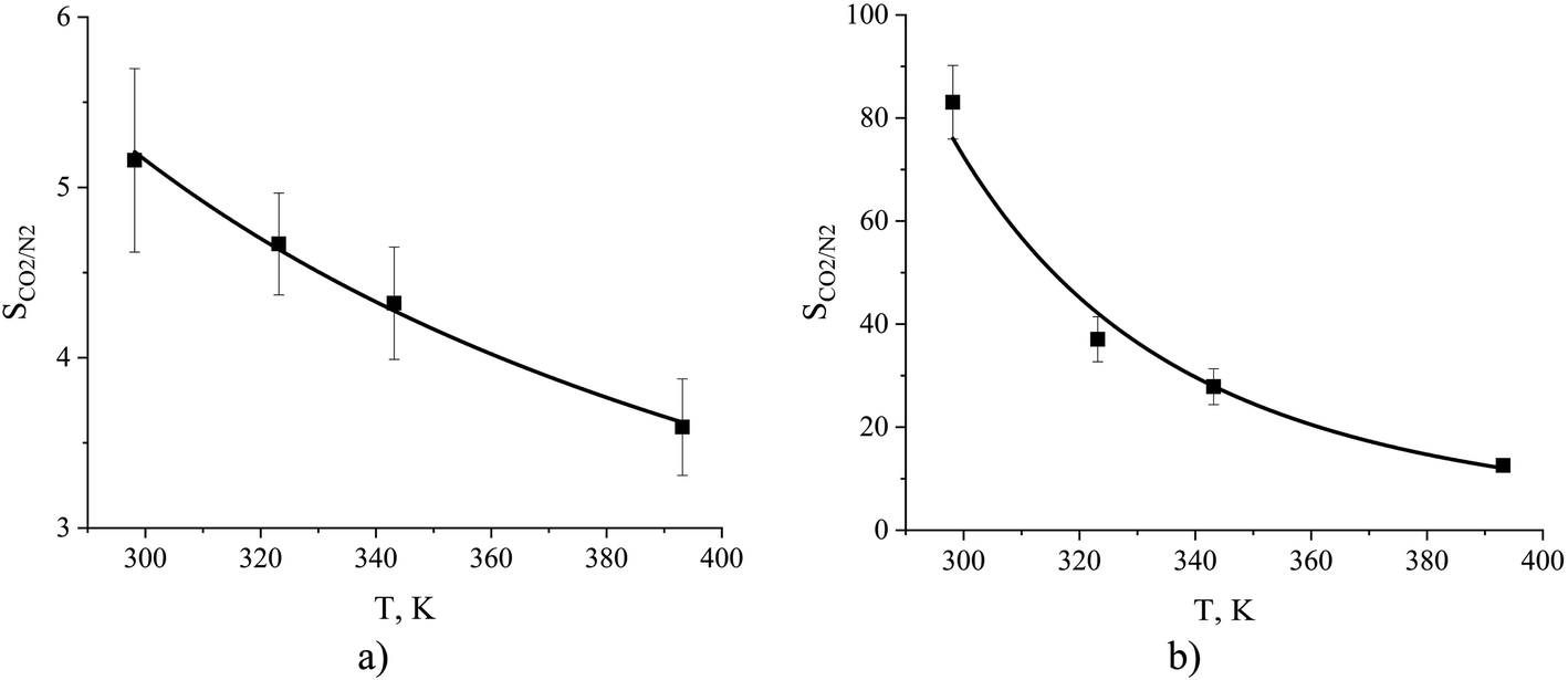 | ||
Fig. 16 Ideal gas CO2/N2 selectivity of (a) the surface and (b) the bulk volume of an ionic liquid film, [BMIM]+[PF6]−, as a function of temperature. The black curves are obtained from eqn (12) combined with a standard definition of ideal selectivity, e.g. . . | ||
In Table S9 of the ESI,† we summarize values of all key properties obtained in this study including the Henry's constants, equipartition thicknesses, and selectivities for the processes of carbon dioxide and nitrogen adsorption and absorption in the ionic liquid, [BMIM]+[PF6]−, from binary gas mixtures (Table S1†).
3.3. A predictive model of gas adsorption and absorption in thin films of ionic liquids
Having discussed competitive behavior of gas adsorption and absorption in films of ionic liquid and defined the equipartition thickness which characterizes this competition, we propose a predictive model of gas adsorption in supported ionic liquid phases.The principles of the model are illustrated in Fig. 17. The model is based on the key assumption that the ionic liquid is uniformly distributed on the surface of the mesoporous material substrate. In the first step of the construction of the model, we collect the required data on the structure of the porous material with and without the ionic liquid. This data is obtained using the standard nitrogen or argon physical adsorption characterization methods. The data includes the surface area and the volume of the pristine material and the surface area and the volume of the material impregnated with the ionic liquid. From the difference in the cumulative pore volumes of the pristine and impregnated materials, one can obtain the volume of the ionic liquid inside the pores, as schematically depicted in Fig. 17. If we assume that the density of the ionic liquid remains close to the bulk value and knowing the surface area of the support material, we can estimate the average thickness of the film.
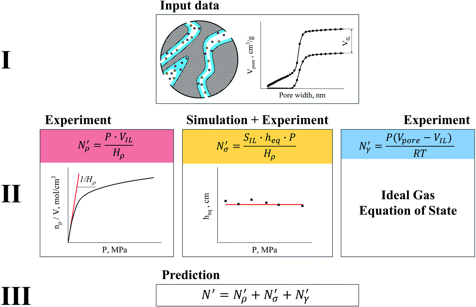 | ||
Fig. 17 Diagram showing how different contributions to the absolute amount of gas are obtained from experimental and simulation data and used to predict the gas capacity of SILP materials. Stage I: the schematic illustrates the structure of the mesoporous material (shaded area) impregnated with a uniformly distributed ionic liquid (blue area) with the surface area SIL, cm2 g−1 of sample, and the gas phase absorbed in the liquid phase (red circles), adsorbed on the surface (yellow circles), and present in the bulk gas phase (dark blue circles); the plot depicts the cumulative pore volume, Vpore, cm3 g−1 of sample, for a pristine porous material (black squares) and the same material containing an ionic liquid (black circles) of volume, VIL, cm3 g−1 of sample. Stage II: the plot on the left is the absorption isotherm for a gas of interest dissolved in the ionic liquid at a particular temperature and showing the definition of the Henry's constant; the plot in the center shows the equipartition thickness (single black data points) as a function of pressure at a particular temperature, where the red line is the constant value obtained from eqn (8); the inset on the right is the ideal gas equation of state. The amount of gas absorbed in the liquid phase,  , adsorbed on the surface, , adsorbed on the surface, 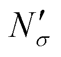 , and present in the bulk gas phase, , and present in the bulk gas phase, 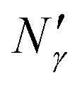 , are per unit mass of the porous sample, thus the total amount N′ and individual contributions have units of mol per g of sample. The formulae above each property in Stage II show the actual calculation required to obtain it. , are per unit mass of the porous sample, thus the total amount N′ and individual contributions have units of mol per g of sample. The formulae above each property in Stage II show the actual calculation required to obtain it. | ||
In the next series of steps (shown as stage II in Fig. 17) we assemble information on various contributions to the total amount adsorbed. As an input, the model requires temperature, pressure and the composition of the gas phase. First, knowing the volume of the ionic liquid in the material, we can estimate the amount of gas absorbed. In the low pressure regime, this requires only knowledge of the Henry's solubility constant at a specific temperature. This data is already available for many gases and ionic liquids, or it can be obtained in an additional experimental measurement. In the formula employed in Fig. 17, Henry's constant has units of (cm3 MPa mol−1), pressure P of (MPa) and ionic liquid volume VIL per unit mass of the sample of (cm3 g−1) resulting in the total amount absorbed  being in units of (mol g−1).
The excess amount adsorbed in terms of the excess number density σ is obtained directly from the simulations, given the conditions specified above. As has been discussed before, the unit of this property employed so far is the number of molecules per unit area of the film. Conversion of this property to the units consistent with  simply requires the area of the material in the appropriate units,
 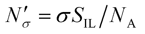 , where SIL is the area per unit mass of the sample in (cm2 g−1) and NA is the Avogadro number.
If the equipartition thickness is not a function of pressure or composition, as emerged here for carbon dioxide, a further simplification is possible. In this case, only one simulation is required to obtain the excess amount adsorbed for all pressures and compositions of interest. This single simulation is used to obtain the value of the equipartition thickness and once it is known, excess adsorption at other conditions is obtained using the equation in Fig. 17 for  , which follows from eqn (8). In this formula, for the sake of consistency, pressure P is in (MPa), heq is in (cm), bulk solubility Henry's constant is in (cm3 MPa mol−1), and area in (cm2 g−1), giving the
  in the consistent units of (mol g−1).
The remaining porous space Vpore − VIL in (cm3 g−1) is occupied by the gas mixture, and the amount of gas can be obtained using an equation of state, for example the ideal gas equation of state. This is illustrated in the final box on the right of stage II of the process, in Fig. 17.
Finally, the three constituent amounts sum to the total amount of the gas component in the SILP system as shown in stage III, in Fig. 17.
Under the assumptions stated above, according to the diagram in Fig. 17, the equipartition thickness can be used to design materials with a controlled contribution from the bulk and interfacial properties of the film of ionic liquid (Fig. 12). For example, for cyclic adsorption processes where fast diffusion of gas species and the amount adsorbed both play a major role, porous materials featuring a layer of ionic liquid of the thickness lower than the equipartition thickness should be most efficient in practice. This particular case can be employed in catalysis where a support with catalytically active centers on the surface is coated with a thin film of IL; or a neutral support is covered with a task-specific ionic liquid containing active moieties.1 On the other hand, for gas separation processes where gas selectivity is among the properties defining the applicability of the material, one should attempt to impregnate a sufficient amount of ionic liquid into the free pore volume such that the layer is thicker than the equipartition thickness or that the pores are completely filled as supported by Shi and Sorescu.37 The advantage of using the equipartition thickness is that it interconnects experimentally measurable (bulk Henry's constant) and non-measurable (the excess amount adsorbed as defined in this article) adsorption properties of materials.
4. Conclusions
The objective of this work was to develop a molecular-level understanding of gas adsorption on the surface of ionic liquids in the context of supported ionic liquid phase materials and their applications for gas separation. For this, we have employed MD simulations to study the adsorption behaviour of CO2 and N2 on the surface of the ionic liquid, [BMIM]+[PF6]−.An important aspect in developing an accurate picture of the adsorption process on the surface and absorption in the bulk volume of the film is the correct description of the interface between the film and the gas phase; and the correct identification of their location relative to the interface. Our approach is based on producing accurate density profiles for gas and liquid phases using the ITIM methodology. The analysis of the calculated density profiles allows us to locate the position of the gas–liquid interface and, using simple analytical criteria, to calculate the excess amount of gas adsorbed on the surface, the amount dissolved in the bulk liquid phase and the amount present in the remaining pore volume. This approach also generates a wealth of information on the structure of the IL in the vicinity of the interface, which can be exploited in engineering ILs with bespoke gas separation properties.
The results show that competition between gas adsorption on the surface and absorption in the liquid phase can be characterized quantitatively by a parameter called the equipartition thickness. The equipartition thickness corresponds to the thickness of the liquid film such that the amount of gas dissolved in the bulk volume is equal to the excess amount adsorbed on the surface. Thus, it directly estimates the contribution from bulk and interfacial properties, which is particularly important in designing novel supported liquid phase class of materials.
At a given temperature, the equipartition thickness is a constant for a particular gas, meaning that it does not depend on the partial pressure of the gas phase if the gas behaviour obeys Henry's law for both adsorption and absorption processes. The definition of the equipartition thickness suggests that it should have low values for gases that are highly soluble in the liquid phase, such as 2.5 nm for CO2 in [BMIM]+[PF6]− at 298 K, and large values for gases with low solubility and strong affinity towards the gas–liquid interface, for example, 41 nm for N2 in [BMIM]+[PF6]− at 298 K in the low pressure limit. We also provided a thermodynamic analysis of how equipartition thickness depends on temperature. Based on this information and experimental data from the literature, we, for the first time, quantitatively estimated the enthalpy and entropy of gas adsorption on the surface of the ionic liquid. These properties provide important insights into the mechanism of gas adsorption, absorption and transition from the surface to the bulk liquid phase.
Another effect explored in this study is the influence of the interface on CO2/N2 selectivity of the film of the ionic liquid. Our analysis reveals that the interface significantly lowers the bulk selectivity of the film from 83 to 5.2 at 298 K as the thickness of the film reduces to a monolayer of the IL. Moreover, the gas selectivity of films follows the same exponentially decreasing trend with temperature as the equipartition thickness. In the Henry's law regime for both gases, the detrimental influence of the interface on selectivity is strong enough that it is not possible to achieve bulk-like selectivity for any reasonable thickness of the film deposited on the surface of a porous material. This aspect may become a limiting factor in the application of supported ionic liquid films in situations requiring high selectivity towards one of the components of the gas phase.
Pressure independence of the equipartition thickness in the Henry's law regime implies that we can use its value together with the experimentally measured gas solubility in the bulk liquid volume at the specified temperature to estimate the excess properties of the interface at any composition and low pressure. This opens an opportunity to propose a predictive model for absolute gas adsorption in supported ionic liquid systems. Indeed, we speculate that given the surface area and pore volume of the mesoporous solid, composition of the gas phase and pressure, and estimated thickness of the IL film, the absolute amount of gas adsorbed can be predicted from the experimentally measured bulk solubility at the same temperature and the equipartition thickness constant, obtained from molecular simulations. This model, however, is based on several significant assumptions: it assumes that the IL is uniformly distributed throughout the material as a film; the support has a negligible effect on the adsorptive properties of the film; the bulk gas phase is ideal, adsorption and absorption processes obey Henry's law. These assumptions need further investigation and validation. In particular, testing the model requires a material prepared with very controlled surface composition and structure. Moreover, the support plays a significant role in the structuring of the liquid phase, especially when the thickness of the film does not exceed a few nanometres.13 Therefore, an additional complexity in adsorption characterization may emerge in these gas–liquid–solid systems.37 Preliminary attempts to prepare a proper sample and to test the model are challenging and require further systematic investigation, which will be pursued in future studies.
Conflicts of interest
There are no conflicts to declare.Acknowledgements
This work was supported by the Edinburgh Global Research Scholarship and the Principal's Career Development PhD Scholarship. This work has made use of the resources provided by the Edinburgh Compute and Data Facility (ECDF) (http://www.ecdf.ed.ac.uk/). Eleanor E. B. Campbell acknowledges financial support from EPSRC FlexiICCS (EP/N024613/1). We also thank Dr Andrei Gromov for invaluable discussions and advice.References
-
R. Fehrmann, A. Riisager and M. Haumann, Supported Ionic Liquids: Fundamentals and Applications, Wiley-VCH, Germany, 2014 Search PubMed
.
- M. E. Boot-Handford, J. C. Abanades, E. J. Anthony, M. J. Blunt, S. Brandani, N. Mac Dowell, J. R. Fernández, M.-C. Ferrari, R. Gross, J. P. Hallett, R. S. Haszeldine, P. Heptonstall, A. Lyngfelt, Z. Makuch, E. Mangano, R. T. J. Porter, M. Pourkashanian, G. T. Rochelle, N. Shah, J. G. Yao and P. S. Fennell, Energy Environ. Sci., 2014, 7, 130–189 RSC
- M. Hasib-ur-Rahman, M. Siaj and F. Larachi, Chem. Eng. Process., 2010, 49, 313–322 CrossRef CAS
- A. Rehman and X. Zeng, RSC Adv., 2015, 5, 58371–58392 RSC
- N. M. Dowell, N. Florin, A. Buchard, J. Hallett, A. Galindo, G. Jackson, C. S. Adjiman, C. K. Williams, N. Shah and P. Fennell, Phys. Chem. Chem. Phys., 2010, 12, 1–28 RSC
- M. B. Sweatman, Chem. Eng. Sci., 2010, 65, 3907–3913 CrossRef CAS
- A. Sharma, C. Julcour, A. A. Kelkar, R. M. Deshpande and H. Delmas, Ind. Eng. Chem. Res., 2009, 48, 4075–4082 CrossRef CAS
- M. E. Perez-Blanco and E. J. Maginn, J. Phys. Chem. B, 2010, 114, 11827–11837 CrossRef CAS PubMed
- M. E. Perez-Blanco and E. J. Maginn, J. Phys. Chem. B, 2011, 115, 10488–10499 CrossRef CAS PubMed
- M. T. Heinze, J. C. Zill, J. Matysik, W. D. Einicke, R. Gläser and A. Stark, Phys. Chem. Chem. Phys., 2014, 16, 24359–24372 RSC
- R. Hayes, G. G. Warr and R. Atkin, Phys. Chem. Chem. Phys., 2010, 12, 1709–1723 RSC
- R. G. Horn and J. N. Israelachvili, J. Chem. Phys., 1981, 75, 1400–1411 CrossRef CAS
- S. Perkin, Phys. Chem. Chem. Phys., 2012, 14, 5052–5062 RSC
- M. V. Fedorov and R. M. Linden-Bell, Phys. Chem. Chem. Phys., 2012, 14, 2552–2556 RSC
- M. Sha, F. Zhang, G. Wu, H. Fang, C. Wang, S. Chen, Y. Zhang and J. Hu, J. Chem. Phys., 2008, 128, 134504–134507 CrossRef PubMed
- R. Atkin and G. G. Warr, J. Phys. Chem. C, 2007, 111, 5162–5168 CrossRef CAS
- M. Haumann, A. Schonweiz, H. Breitzke, G. Buntkowsky, S. Werner and N. Szesni, Chem. Eng. Technol., 2012, 35, 1421–1426 CrossRef CAS
- S. Brunauer, P. H. Emmett and E. Teller, J. Am. Chem. Soc., 1938, 60, 309–319 CrossRef CAS
- F. Heym, W. Korth, J. Thiessen, C. Kern and A. Jess, Chem. Ing. Tech., 2015, 87, 791–802 CrossRef CAS
- N. V. Reichhardt, R. Guillet-Nicolas, M. Thommes, B. Klösgen, T. Nylander, F. Kleitz and V. Alfredsson, Phys. Chem. Chem. Phys., 2012, 14, 5651–5661 RSC
- J. R. Roscioli and D. J. Nesbitt, J. Phys. Chem. Lett., 2010, 1, 674–678 CrossRef CAS
- T. Yan, S. Li, W. Jiang, X. Gao, B. Xiang and G. A. Voth, J. Phys. Chem. B, 2006, 110, 1800–1806 CrossRef CAS PubMed
- M. Klähn and A. Seduraman, J. Phys. Chem. B, 2015, 119, 10066–10078 CrossRef PubMed
- M. B. Shiflett and E. J. Maginn, AIChE J., 2017, 63, 4722–4737 CrossRef CAS
- M. B. Shiflett, A. M. S. Niehaus and A. Yokozeki, J. Phys. Chem. B, 2011, 115, 3478–3487 CrossRef CAS PubMed
- M. B. Shiflett, A. M. S. Niehaus and A. Yokozeki, Sep. Sci. Technol., 2012, 47, 411–421 CrossRef CAS
- M. B. Shiflett, D. J. Kasprzak, C. P. Junk and A. Yokozeki, J. Chem. Thermodyn., 2008, 40, 25–31 CrossRef CAS
- A. Yokozeki, M. B. Shiflett, C. P. Junk, L. M. Grieco and T. Foo, J. Phys. Chem. B, 2008, 112, 16654–16663 CrossRef CAS PubMed
- M. B. Shiflett, B. A. Elliott, S. R. Lustig, S. Subramaniam, M. S. Kelkar and A. Yokozeki, ChemPhysChem, 2012, 13, 1806–1817 CrossRef CAS PubMed
- S. Zeng, X. Zhang, L. Bai, X. Zhang, H. Wang, J. Wang, D. Bao, M. Li, X. Liu and S. Zhang, Chem. Rev., 2017, 117, 9625–9673 CrossRef CAS PubMed
- P. Scovazzo, J. Kieft, D. A. Finan, C. Koval, D. DuBois and R. Noble, J. Membr. Sci., 2004, 238, 57–63 CrossRef CAS
- A. I. Akhmetshina, N. R. Yanbikov, A. A. Atlaskin, M. M. Trubyanov, A. Mechergui, K. V. Otvagina, E. N. Razov, A. E. Mochalova and I. V. Vorotyntsev, Membranes, 2019, 9(9), 1–14 Search PubMed
- Y. J. Ban, Z. J. Li, Y. S. Li, Y. Peng, H. Jin, W. M. Jiao, A. Guo, P. Wang, Q. Y. Yang, C. L. Zhong and W. S. Yang, Angew. Chem., Int. Ed., 2015, 54, 15483–15487 CrossRef CAS PubMed
- H. Li, L. Tuo, K. Yang, H.-K. Jeong, Y. Dai, G. He and W. Zhao, J. Membr. Sci., 2016, 511, 130–142 CrossRef CAS
- J. M. Vicent-Luna, J. J. Gutierrez-Sevillano, J. A. Anta and S. Calero, J. Phys. Chem. C, 2013, 117, 20762–20768 CrossRef CAS
- S. Zhang, J. Zhang, Y. Zhang and Y. Deng, Chem. Rev., 2017, 117, 6755–6833 CrossRef CAS PubMed
- W. Shi and D. C. Sorescu, J. Phys. Chem. B, 2010, 114, 15029–15041 CrossRef CAS PubMed
- L. B. Partay, G. Hantal, P. Jedlovszky, A. Vincze and G. Horvai, J. Comput. Chem., 2008, 29, 945–956 CrossRef CAS PubMed
- B. Doherty, X. Zhong, S. Gathiaka, B. Li and O. Acevedo, J. Chem. Theory Comput., 2017, 13, 6131–6145 CrossRef CAS PubMed
- M. J. Abraham, T. Murtola, R. Schulz, S. Páll, J. C. Smith, B. Hess and E. Lindahl, SoftwareX, 2015, 1–2, 19–25 CrossRef
- L. Martínez, R. Andrade, E. G. Birgin and J. M. Martínez, J. Comput. Chem., 2009, 30, 2157–2164 CrossRef PubMed
- D.-Y. Peng and D. B. Robinson, Ind. Eng. Chem. Fundam., 1976, 15, 59–64 CrossRef CAS
- G. Bussi, D. Donadio and M. Parrinello, J. Chem. Phys., 2007, 126, 014101 CrossRef PubMed
- C. G. Aimoli, E. J. Maginn and C. R. A. Abreu, J. Chem. Phys., 2014, 141, 134101–134113 CrossRef CAS PubMed
- J. J. Potoff and J. I. Siepmann, AIChE J., 2001, 47, 1676–1682 CrossRef CAS
- M. Jorge, P. Jedlovszky and M. N. D. S. Cordeiro, J. Phys. Chem. C, 2010, 114, 11169–11179 CrossRef CAS
- M. Jorge, G. Hantal, P. Jedlovszky and M. N. D. S. Cordeiro, J. Phys. Chem. C, 2010, 114, 18656–18663 CrossRef CAS
- G. Hantal, I. Voroshylova, M. N. D. S. Cordeiro and M. Jorge, Phys. Chem. Chem. Phys., 2012, 14, 5200–5213 RSC
- G. Hantal, M. Sega, S. Kantorovich, C. Schroder and M. Jorge, J. Phys. Chem. C, 2015, 119, 28448–28461 CrossRef CAS
- G. Yu, D. Zhao, L. Wen, S. Yang and X. Chen, AIChE J., 2012, 58, 2885–2899 CrossRef CAS
- G. Hantal, M. N. D. S. Cordeiro and M. Jorge, Phys. Chem. Chem. Phys., 2011, 13, 21230–21232 RSC
-
J. W. Gibbs, Collected works, Yale University Press, New Haven, vol. 1, 1961 Search PubMed
-
E. A. Guggenheim, Thermodynamics, Interscience Publishers, Inc., New York, 2nd edn, 1967 Search PubMed
- C. J. Radke, Adv. Colloid Interface Sci., 2015, 222, 600–614 CrossRef CAS PubMed
- L. Sarkisov and A. Harrison, Mol. Simul., 2011, 37, 1248–1257 CrossRef CAS
- M. Lísal and P. Izak, J. Chem. Phys., 2013, 139, 014704–014715 CrossRef PubMed
- K. Nakajima, S. Nakanishi, M. Lísal and K. Kimura, J. Chem. Phys., 2016, 144, 114702–114706 CrossRef PubMed
-
K. Wandelt, Surface and Interface Science, Germany, WILEY-VCH, 2020 Search PubMed
- K. Nakajima, S. Nakanishi, Z. Chval, M. Lísal and K. Kimura, J. Chem. Phys., 2016, 145, 184704–184706 CrossRef PubMed
- K. Nakajima, S. Nakanishi, M. Lísal and K. Kimura, J. Mol. Liq., 2017, 230, 542–549 CrossRef CAS
- M. Sega, B. Fábián and P. Jedlovszky, J. Chem. Phys., 2015, 143, 114709 CrossRef PubMed
- A. L. Myers and P. A. Monson, Adsorption, 2014, 20, 591–622 CrossRef CAS
- J. L. Anthony, E. J. Maginn and J. F. Brennecke, J. Phys. Chem. B, 2002, 106, 7315–7320 CrossRef CAS
- J. Jacquemin, P. Husson, V. Majer and M. F. Costa Gomes, Fluid Phase Equilib., 2006, 240, 87–95 CrossRef CAS
- I. Langmuir, J. Am. Chem. Soc., 1918, 40, 1361–1403 CrossRef CAS
-
S. I. Sandler, Chemical, Biochemical, and Engineering Thermodynamics, 5th edn, Wiley, 2017 Search PubMed
-
J. M. Prausnitz, R. N. Lichtenthaler and E. Gomes de Azevedo, Molecular Thermodynamics of Fluid-Phase Equilibria, Prentice Hall, New Jersey, 3d edn, 1999 Search PubMed
- NIST Chemistry WebBook, https://webbook.nist.gov; accessed February, 2020 Search PubMed.
- Z. Lei, C. Dai and B. Chen, Chem. Rev., 2014, 114, 1289–1326 CrossRef CAS PubMed
- A. Finotello, J. E. Bara, D. Camper and R. D. Noble, Ind. Eng. Chem. Res., 2008, 47, 3453–3459 CrossRef CAS
- P. Husson-Borg, V. Majer and M. F. Costa Gomes, J. Chem. Eng. Data, 2003, 48, 480–485 CrossRef CAS
- J. Kumełan, Á. Pérez-Salado Kamps, I. Urukova, D. Tuma and G. Maurer, J. Chem. Thermodyn., 2005, 37, 595–602 CrossRef
- S. Raeissi, L. J. Florusse and C. J. Peters, J. Chem. Eng. Data, 2011, 56, 1105–1107 CrossRef CAS
- M. F. Costa Gomes, J. Chem. Eng. Data, 2007, 52, 472–475 CrossRef
Footnote |
| † Electronic supplementary information (ESI) available. See DOI: 10.1039/d0ta03419c |
| This journal is © The Royal Society of Chemistry 2020 |