 Open Access Article
Creative Commons Attribution 3.0 Unported Licence
Aging of living polymer networks: a model with patchy particles
Stefano
Iubini
 *ab,
Marco
Baiesi
bc and
Enzo
Orlandini
bc
aConsiglio Nazionale delle Ricerche, Istituto dei Sistemi Complessi, via Madonna del Piano 10, I-50019 Sesto Fiorentino, Italy. E-mail: stefano.iubini@fi.isc.cnr.it
bDipartimento di Fisica e Astronomia, Università di Padova, Via Marzolo 8, I-35131 Padova, Italy
cINFN, Sezione di Padova, Via Marzolo 8, I-35131 Padova, Italy
First published on 24th September 2020
Abstract
Microrheology experiments show that viscoelastic media composed by wormlike micellar networks display complex relaxations lasting seconds even at the scale of micrometers. By mapping a model of patchy colloids with suitable mesoscopic elementary motifs to a system of worm-like micelles, we are able to simulate its relaxation dynamics, upon a thermal quench, spanning many decades, from microseconds up to tens of seconds. After mapping the model to real units and to experimental scission energies, we show that the relaxation process develops through a sequence of non-local and energetically challenging arrangements. These adjustments remove undesired structures formed as a temporary energetic solution for stabilizing the thermodynamically unstable free caps of the network. We claim that the observed scale-free nature of this stagnant process may complicate the correct quantification of experimentally relevant time scales as the Weissenberg number.
1 Introduction
Many soft materials with important industrial and medical applications are formed by thermodynamic self-assembly of elementary constituents dispersed in aqueous solution.1 This process gives rise to networks of linear or branched fibers or even more complex objects2 that can continuously break, rejoin or get entangled. These “living” materials3 have remarkable viscoelastic properties that are typically studied either by imposing a shear stress with a rheometer1,4 or by dragging a micro-sized probe through the medium as in active microrheology.5,6 The response and relaxation dynamics of living polymers are the result of large-scale reorientation and mutual reptation of the fibers that, in turn, depend on small scales mechanisms such as scission and rewiring of branches. This multiscale process can give rise to global relaxation dynamics that, for systems as wormlike micelles, has been measured to be of the order of seconds.5,6An important issue is the relation between the macroscopic dynamical response of the system, measured experimentally, and its less accessible local structural rearrangements. From the theoretical side, mean-field theories and microscopic constitutive models have been successfully developed3,7–10 to rationalize the outcomes of rheological experiments. However, these studies often dealt with small temperature jumps, which may not lead to the significant disturbance of the micellar networks as, e.g., in microrheological experiments at large Weissenberg numbers where a microbead is moved in the medium at high velocities.11,12 At the same time, numerical studies,13–18 performed at a coarse-grained molecular level on specific systems (cationic cylindrical micelles and cetyltrimethylammonium chloride micelles) have either looked at the competition between shear flow and internal network dynamics or estimated the strands scission and branching free energies of these systems. However, these models, being still quite detailed and system-specific, cannot have access to the scales spanned by rheological experiments (of the order of seconds and above μm3) or address universal features of the phenomenon.
A generic understanding of the transient behavior of living polymers can be sought by addressing the following questions: which are the dominant local structures (or “microstates”) that compete dynamically in the rearrangement of a relaxing living random network? How does the long-time relaxation depend on the mechanisms of local rewiring and scission of the fibers? Is the time dependence of relevant observables undergoing relaxation characterized by simple exponentials or is it more similar to a dynamical scaling with power laws? Simulations of coarse grained models at mesoscopic level are an ideal tool for answering these questions: they allow a direct investigation both at short/small and long/large scales and they may adopt a well controlled protocol for driving the system out of equilibrium.
In this paper, we introduce a simple, coarse-grained, description of a thermally driven self-assembly process generating a living network of fibers by means of the merging, scission and rewiring of basic units that represent a portion of the tubular structure. These units are described by patchy particles.19–33
By using large-scale Brownian dynamic simulations and analytical arguments to estimate the free-energy barriers between the competing “microstates”, we characterize the underlying microscopic dynamics that leads to the global relaxation towards the formation of the random networks. To go beyond the regime of small perturbations a wide temperature quench is imposed on the system.
The paper is organized as follows. In Section 2 we introduce the coarse-grained model and the numerical set-up. In Section 3 we analyze the thermodynamic and kinetic properties of local motifs and their effect on the large-scale relaxation dynamics of the system upon a temperature quench towards a self-assembled equilibrium state. Section 4 is devoted to a final discussion of the results and to highlight future developments that can be explored within this approach. Finally, the appendix contains the details of the numerical methods employed for this study.
2 Model
The coarse grained model we consider belongs to the vast class of patchy particle models used in literature to study self-assembled structures19 but it is specifically designed to describe living polymer networks and particularly worm-like micelles. Let us first introduce its basic properties in the context of patchy colloids (Section 2.1) and later discuss a more specific connection with micellar systems (Section 2.2).2.1 Patchy colloids
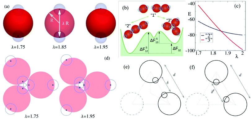
The elementary unit of our coarse-grained description is a rigid body consisting of three sub-units: there is a central core of radius R (red spheres in Fig. 1(a)) and two radially opposite (i.e., antipodal) “patches” or “sticky spots” (blue transparent spheres) fixed at distance λR. The effective interaction between units is the sum of two contributions: a steric (excluded volume) interaction between the core beads and a mutual attraction between patches belonging to different rigid bodies. The first is accounted for a shifted and truncated Lennard-Jones potential with characteristic amplitude ε and range R. Patch–patch attraction, that would lead to the aggregation of units at sufficiently low temperatures, is instead described by a truncated Gaussian potential with range σ = 0.4R and amplitude A = 40ε (this amplitude allows to recover free energies at T ≈ 1 that are comparable to the ones measured in micellar systems), see Appendix A for more details.Two main characterizing aspects of our model are worth noticing. First, in most of the patchy colloids models19 the branching points of the assembled structures are generated either by introducing a fraction of colloids decorated by three or more attractive patches20,21 or by allowing for different types of patch–patch interactions.22–25 In either case, a better control of the phase diagram is achieved by satisfying a single-bond-per-patch condition.26 In our model only bifunctional patchy beads are considered and the local branching emerges naturally from the formation of multiple contacts between patchy particles. Note that similar systems were studied experimentally27 and numerically28–30 (see also some more recent work31–33). The second aspect concerns the presence of the tunable branching parameter λ. This has been introduced to mimick the propensity of worm-like micelles to branch as a function of salt concentration (see Section 2.2). In particular, by varying λ ≤ 2 (λ = 2 corresponds to standard surface interactions between patches), one can change the depth of the sticky spots within the repulsive core and hence bias the system towards the formation of either linear strands or branches (see Fig. 1(b) for the simplest case of trimers). More precisely, for large values of λ the units tend to form “vertex” or “3 contact” states (see Fig. 1(b)) rather than the “strands” or “2 contact” states.
This behavior can be explained quantitatively by minimizing analytically the total potential energy of the vertex and strand configurations of a trimer, see Fig. 1(c). As a matter of fact, we find that the formation of strands is energetically advantageous with respect to branch points only for sufficiently small values of λ. Branch points become instead energetically more convenient if λ gets close enough to 2. For example, in the two situations represented in Fig. 1(d), for λ = 1.75 the mutual attraction between sticky spots take place at a distance larger than the interaction range σ, reducing the stability of the trimer, while for λ = 1.95 the three pairs of sticky spots are all at a distance within σ and thus very stable.
The effect of the branching parameter λ can be further rationalized as follows. Let us focus on a linear dimer (see Fig. 1(e)) in its mechanical equilibrium position with bond energy ul < 0 determined by the distance d between unit centers and the distance δ = d − λ between sticky centers. The branched configuration can be obtained by rotating the two reference units by angles of 30° with respect to their centers on the plain containing the trimer (Fig. 1(f)). In this rotated configuration the two sticky spots increase their distance δ′ > δ thus decreasing their attracting force, while the repulsive centers of the units are not modified significantly. Since δ′ > δ the single bond energy ub > ul. However, due to the different number of bonds in branched and linear trimers, the overall energy of the branched trimer Eb = 3ub can be lower and thus more stable than the linear trimer configuration with energy El = 2ul. This takes place if λ is large enough to keep δ′ within the range of attraction of the sticky spots. Upon decreasing λ, one meets a situation in which δ′ is longer than the range of attraction between sticky spots and hence the branched configuration becomes less stable than the linear one.
2.2 Wormlike micelles
The patchy colloid model described above is rather generic but it can be specialised on worm-like micelles for which a wealth of experimental data is nowadays available. In this context, it is known that the spatial organization of micelles in spherical, linear or branched structures depends on several parameters such as salt concentration3,16 or the spontaneous curvature of surfactants.34,35 This feature makes large-scale numerical simulations rather challenging, even at coarse-grained level, since a detailed description of micelles recombination dynamics requires to resolve the mutual interaction of solvent, salt and surfactant particles at the subnanometric length scales.16,18 In contrast, in our minimal model the effect of ionic particles and curvature is taken into account effectively through the tunable branching parameter λ.In this approach an ensemble of surfactants forming a globular micelle or the segment of a wormlike network, as those sketched in Fig. 2, is mapped to a single micellar unit. In this context, one may think of λ as a parameter describing the strength of salt concentration. This is indeed known to shrink the effective size of the hydrophilic heads of the surfactants, thus favoring the appearance of structures with negative surface curvature as hubs in the micellar network.
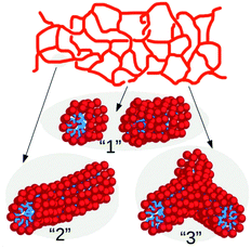 | ||
| Fig. 2 Sketch of a wormlike micellar network and of selected portions where each surfactant is depicted as a hydrophilic (red) head and a hydrophobic (blue) tail. The numbering of the network portions follows that of the corresponding patchy particle states of Fig. 1(b). | ||
Note that the resolution of our coarse grained model cannot describe effects below the size of a globular micelle. In particular, unlike previous models,13–18 the dynamics of a single surfactant is not included in our description. On the other hand, the fact that the basic element of our model is not representing a single surfactant but rather a collection (i.e., some dozens) of them, should not affect the large scale dynamics of the network structure that we aim to explore here.
2.3 Simulations
The dynamics of the system follows a set of coupled Langevin equations for the interacting units in an implicit solvent at fixed volume and constant temperature T (henceforth measured in units of ε, with Boltzmann constant kB = 1 and ε = 1). Numerical simulations are performed with LAMMPS engine.36 For a more detailed description of the model and for a mapping of the simulation units to those of a wormlike micellar system, see the appendix.By assuming, for instance, that the core radius of the elementary unit length is of the order of the average width measured in wormlike micelles, i.e., R ≈ 5 nm, the largest box considered in our simulations with dimensions 108R × 108R × 324R maps to a system volume ≈0.5 μm3. Moreover, our runs simulate systems of up to N = 6000 units; this would correspond to a number of molecules of surfactants of the order of 105.37 Finally, since the simulation time unit τ is mapped to 2 μs in the real system (see appendix), the longest simulation time we can reach, t = 107τ, corresponds approximately to 20 s and is comparable with the duration of recent experiments.6,38 Simulations are performed with an integration time step equal to 10−2τ. We have verified that this time step suffices to ensure suitable numerical accuracy in all regimes considered in this study.
We describe the time evolution of the network by monitoring the formation/disappearance of its local motifs, such as dangling ends and branched structures. These are classified by looking at the number of contacts shared by their patches. A sticky spot is defined to share a contact with another one if the distance between their centers is ≤R, see appendix for further details. A dangling end contains a unit with k = 1 contacts, while each branch “3” contains three units each with k = 3 contacts, when they are part of a strand in the network (that is, a chain of elementary units with k = 2) which ends either with dangling ends or branching points. Finally, we define the length L of a strand as the total number of linear bonds between its extrema. For example, a dimer composed of two units with k = 1 has length L = 1, while a sequence on five units with k = 2 between two joints has length L = 6. We assign L = 0 to isolated units (k = 0).
3 Results
3.1 Thermodynamics and scission time of local motifs
We first analyze the equilibrium thermodynamics of the smallest motifs assembled in the network, namely the strands and the branch points (respectively state “2” and “3” in Fig. 1(b)). In presence of thermal fluctuations, the zero-temperature scenario of Fig. 1(c) is modified by entropic contributions and a comparison between the free energies F of the microstates “2” and “3” must be performed. Note that in micellar solutions thermal fluctuations not only determine the configurational entropy of the motifs, but also modify the typical energies of strand and branch points.35 At our coarse-graining level, this would result to a branching parameter λ that depends also on temperature. In this study, however, since we are interested in identifying the role of purely entropic contributions, T and λ are tuned independently. On the other hand, once the model is fully characterized, any mapping to a given experimental condition of salt concentration and temperature can be obtained through a suitable selection of the λ and T values.To estimate the free energy difference ΔF32 = F3 − F2 we have carried out Langevin simulations with parallel tempering sampling technique39,40 on a system with three units confined within a small fixed volume (see appendix for details). In Fig. 3(a) we report ΔF32 as a function of T for four values of λ. It displays a linear growth with T, with an intercept at T = 0 that matches quite well the energy differences found analytically from Fig. 1(c), see open symbols. Entropy differences ΔS32 are thereby identified by the (negative) slope ∂ΔF32/∂T, see dashed lines. Note that the combination of the negative entropy gap ΔS32 with a λ-dependent energy potential may result in a situation where the most favorable thermodynamic state is T-dependent, as for λ = 1.95, where branch points are stable only at low T. Analogous results involving temperature-dependent effective valence were previously found in particles models with explicit dissimilar patches.23 These findings match the prediction18 that wormlike micelles may form networks with a variety of features, depending on the inclination of their tubular structures to branch.
 | ||
| Fig. 3 Thermodynamic and kinetic properties of a trimer. (a) Free energy difference ΔF32vs. temperature T for λ = 1.75, 1.79, 1.86 and 1.95. For the same values, −ΔS32 = 2.4, 3.2, 3.2 and 5.1 from linear fits, see dashed lines. Open symbols reported on the vertical axis correspond to the energy difference from Fig. 1(c), at T = 0. (b) Average scission time t3 for a trimer initially arranged in the configuration “3” and (c) average scission time t2 for a strand “2”, as a function of the inverse temperature 1/T. Dashed lines are Arrhenius fits of ΔES13 and ΔES12. In all panels different symbols refer to different values of the branching parameter λ (see legend in panel (b)). | ||
To see how local thermodynamic properties affect the dynamics of network formation, we have computed the average scission time either from the strand “2” or from the branch point “3” to the detached dimer-plus-monomer state “1”, see Fig. 1(b). Scission times have been computed from equilibrium simulations for different temperatures T and different values of the branching parameter λ, see appendix for details. They follow a standard Arrhenius law once reported as a function of 1/T. For branched initial configurations (Fig. 3(b)), we find average scission times t3 ∼ exp(ΔES13/T) with energy ΔES13 whose fitted values are ΔES13 ≈ 15, 21, 26, 37 (in units of kBT), respectively for λ = 1.75, 1.79, 1.86, and 1.95. Similarly, the scission times for strand initial configurations is t2 ∼ exp(ΔES12/T) (Fig. 3(c)) and the fitted values of the scission energies ΔES12 are 24, 27, 32, and 29 for the same λ values. Importantly, these values of ΔES12 and ΔES13 are in a range ≈15–35 kBT fully compatible with the current estimates of the scission energies (or enthalpies) of micellar systems.18,38,41,42
3.2 Relaxation dynamics
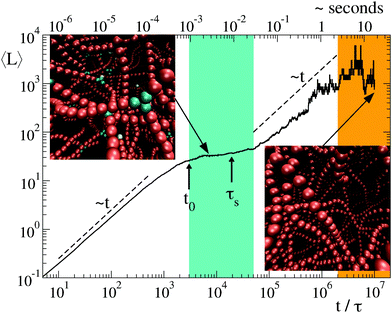
Once clarified the equilibrium and kinetic properties of the basic units of the model, we now turn to the main topic of this work, namely the study of the long time relaxation process of the system towards relatively large networks at equilibrium. This is carried out by large-scale simulations in which the system starts from a solution of freely diffusing globular micelles (which in our model are represented by isolated units and initialised with T ≫ 1). At sufficiently low T, isolated units start to aggregate into intricate networks, see the inset of Fig. 4 and 6(b). Their typical structures bear a strong resemblance of those appearing on smaller scales in less coarse-grained models.13–18 In Fig. 4 we report the time evolution of the mean strand length 〈L〉 for λ = 1.75, T = 1 and N = 6000, where the symbol 〈·〉 indicates the average over all strands found in the system at time t. Note that, for the chosen values of λ and T, equilibrium thermodynamics predicts a large predominance of strands over branching points, see red squares in Fig. 3(a). Hence the system is expected to arrange itself in long strands. However, after a relatively fast power-law growth for a time t0 ∼ 103τ, 〈L〉 reaches first a plateau that lasts for a decade (see cyan band, whose width is τs ∼ 104τ) and then slowly increases as a second power law towards the expected equilibrium value (orange band). From numerical fits, we have found that the exponent of the two power-laws is ≃1, see dashed lines in Fig. 4. The intermediate plateau on τs indicates that the growth of the network cannot be described in terms of a simple coalescence process,43,44 due to the presence of a metastable state characterized by an excess of branching points (see top-left inset in Fig. 4). As a result, longer strands can be progressively assembled by slow rearrangements of the whole structure.The macroscopic relaxation process is further understood by looking at the dynamical evolution of units classified by their contacts. Let Nk be the number of units with k contacts and fk = Nk/N their fraction. Due to the core repulsion, for λ ≲ 2 a unit may establish at most k = 4 contacts (two per side).
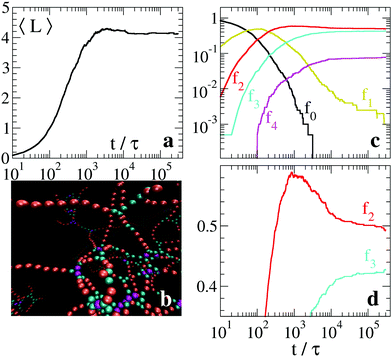
In Fig. 5 we plot the fractions fk vs time for the same system of Fig. 4. After a quick condensation to a network (f0 → 0 for t → t0), the network does not contain the equilibrium proportion of network motifs. The fraction f1 of units at dangling ends tends slowly to zero, with a scaling compatible with a power law f1 ∼ t−1. Eventually, at teq ≈ 2 × 10⁶τ, mapped to ≈10 s, the fraction f1 reaches its asymptotic value. This very slow reduction of the number of strands with dangling ends highlights a stagnant global relaxation of the network. Also the fraction f3 of units meeting at branches slowly decreases as f3 ∼ t−1 till teq and then fluctuates around its equilibrium value. We can approximate the asymptotic ratio ![[f with combining macron]](https://www.rsc.org/images/entities/i_char_0066_0304.gif) 3/
3/![[f with combining macron]](https://www.rsc.org/images/entities/i_char_0066_0304.gif) 2 ≃
2 ≃ ![[f with combining macron]](https://www.rsc.org/images/entities/i_char_0066_0304.gif) 3 (the bar over fk denotes the long-time value of fk) by the equilibrium expression
3 (the bar over fk denotes the long-time value of fk) by the equilibrium expression ![[f with combining macron]](https://www.rsc.org/images/entities/i_char_0066_0304.gif) 3/
3/![[f with combining macron]](https://www.rsc.org/images/entities/i_char_0066_0304.gif) 2 = exp(−Δf32/T), where Δf32 = ΔF32/3 is the free energy difference per unit derived from the single trimer problem, see Section 3.1. For λ = 1.75 and T = 1, this gives
2 = exp(−Δf32/T), where Δf32 = ΔF32/3 is the free energy difference per unit derived from the single trimer problem, see Section 3.1. For λ = 1.75 and T = 1, this gives ![[f with combining macron]](https://www.rsc.org/images/entities/i_char_0066_0304.gif) 3/
3/![[f with combining macron]](https://www.rsc.org/images/entities/i_char_0066_0304.gif) 2 ≃ 0.003. This prediction, however, is not fully quantitative, as it neglects the role of trimer interactions (and even more complex many-body interactions) which are present in the macroscopic system. Finally, a very small amount of units with four contacts (k = 4) is temporarily observed during the relaxation process, in correspondence of the maximum concentration of branches f3. This is not surprising, as four-contacts states arise when the branched geometry affects both sides of a unit. Since their energetic cost is essentially twice the cost of a single branch, their asymptotic concentration is expected to be of the order of (
2 ≃ 0.003. This prediction, however, is not fully quantitative, as it neglects the role of trimer interactions (and even more complex many-body interactions) which are present in the macroscopic system. Finally, a very small amount of units with four contacts (k = 4) is temporarily observed during the relaxation process, in correspondence of the maximum concentration of branches f3. This is not surprising, as four-contacts states arise when the branched geometry affects both sides of a unit. Since their energetic cost is essentially twice the cost of a single branch, their asymptotic concentration is expected to be of the order of (![[f with combining macron]](https://www.rsc.org/images/entities/i_char_0066_0304.gif) 3)2, a behaviour which, however, was not observed in our simulations due to finite size and finite time effects.
3)2, a behaviour which, however, was not observed in our simulations due to finite size and finite time effects.
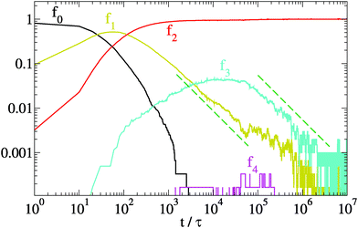 | ||
| Fig. 5 Evolution of the relative density fk of units with k-contacts for the same relaxation dynamics of Fig. 4 (N = 6000, λ = 1.75 and T = 1). Dashed lines represent a scaling ∼t−1. | ||
The slow scalings of f1, f3, and 〈L〉 suggest that the dynamics within the network proceeds through a sequence of frustrated rearrangements. For instance, a dangling end joining its free cap to the side of a strand would form a branch. This local state is however thermodynamically less favorable (see Fig. 1(b)), thus leading to a subsequent decay back to a dangling end and a linear strand. A direct merging of two dangling ends would better stabilize the system but this event becomes more and more unlikely with time due to the concomitant decreases of the dangling ends population. From this argument it follows that the time scale of network rearrangements τs in Fig. 4 is determined by the scission time of branch points. Indeed from Fig. 3(b) we find that t3 ≃ 104 ≃ τs for λ = 1.75 and T = 1.
The variety of micellar structures depends on several parameters (solvent, salt concentration, surfactant chemistry) and includes networks rich in branches. This situation is realized in our model by increasing λ. For example, with λ = 2 and T = 1, the relaxation proceeds through the formation of a metastable network with relatively small average strand length, as shown in Fig. 6(a) (the configuration at the end of the simulation is shown in Fig. 6(b)). Again, there is a very slow convergence of the fraction f1 of units at the caps of dangling ends, see Fig. 6(c). In Fig. 6(d), in linear scale on the vertical axis, it is apparent that also the fractions f2 and f3 are slowly converging toward their asymptotic average values. Here, equilibrium thermodynamics predicts a clear dominance of branches over strands: in the single trimer study in Fig. 3(a), we obtain ΔF32 ≃ −8 for the nearby parameters λ = 1.95 and T = 1. Therefore, we conclude that equilibrium is far from being reached and that the configuration reported in Fig. 6(b) is still a metastable one.
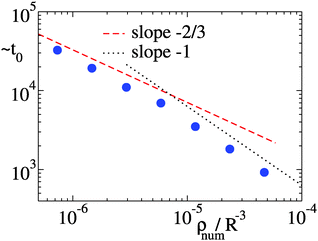
The phenomenology described above holds for several particle densities. Indeed, by changing considerably N and keeping the volume V fixed, we have been able to vary ρnum = N/V by a factor of 3 (data not shown) Yet, the scaling of the mean quantities is quite similar to the previous cases. In particular, the average strand length in the initial metastable network is unaffected by the change of density. However, the density determines the time scale t0 of the initial network condensation. This is defined as the time needed for the fraction of 0-contacts f0 to go below the threshold value f*= 0.4 starting from a homogeneous initial condition of isolated particles (f0 = 1) at time t = 0. By scaling arguments, at low concentrations, diffusion leads to t0 ∼ ρnum−2/3. At higher concentrations it is rather the “ballistic” expansion of the network core (as in other Brownian coagulation systems45) that determines the time scale t0 ∼ ρnum−1. In Fig. 7 we report estimates of ∼t0 (up to a constant that is irrelevant for the scaling) which are compatible with the two regimes, see also the appendix for further details. Note that we have verified that f* is irrelevant for the scaling behavior of t0 with ρnum in so far as f* is large enough to provide a sampling of the initial relaxation stages.
4 Discussion
We have introduced a patchy particle model to study the relaxation dynamics of living polymer networks driven out equilibrium by a deep thermal quench. A novel relevant feature of this coarse-grained description is its ability to bridge the short time dynamics of its elementary motifs (dangling ends, linear strands, branches) with the long time behavior of the mesoscopic network.By combining large-scale simulations and analytical estimates of the free energy barriers between motifs, we rationalize the observed slow convergence of the network to equilibrium in terms of the frustrated dynamics of the local motifs. In particular we argue that the relaxation process develops through a sequence of rearrangements that are not only energetically challenging but also require the solution of topological constraints. Importantly, such constraints do not derive from static functional properties of motifs, but emerge dynamically and depend on local thermodynamic conditions. Moreover, the far-from-equilibrium character of our setup is naturally beyond the perturbative regime, where exponential relaxation laws are expected.7,10
While we have used a standard temperature quench to produce a clean representation of the network relaxation, in practice the considerations we have drawn should be extended to transient regimes of mechanical or chemical origin. For instance, a passage of a micro-bead through a portion of a viscoelastic fluid made of wormlike micellar networks may “scramble” severely the system by generating dangling ends and by distorting the branches. This unbalanced state then should re-equilibrate by following a relaxation dynamics akin to the one we have characterized here. Such scenario is relevant for microbeads of diameter D traveling with mean velocity v at high Weissenberg number Wi = v/vr, where vr = D/τrel is the velocity scale associated to the relaxation over D with time scale τrel. Our findings suggest that a proper definition of τrel should consider the possible emergence of power-law behaviors for strongly disturbed polymer networks. In fact, the relaxation times found here are of the same order of magnitude (seconds) of those measured experimentally in viscoelastic micellar networks.5,6 It is thus natural to conjecture that τrel is the time at which each microscopic motif of the network reaches, through a power-law decay, its typical (equilibrium) fraction. In this respect, it is the ending time of this scale-free aging (not to be confused with chemical aging, as a high-temperature degradation of carbon–carbon double bonds46) that should be considered for evaluating the standard Deborah and Weissenberg numbers used in experiments.11,12
Our findings also raise the question on which of, e.g., self-healing rubber,47,48 colloidal systems,49–51 or network fluids52 do experience a relaxation process characterized by a slow rearrangement of local motifs. In this respect we believe that coarse-grained descriptions based on patchy colloids, as the one presented here, can be highly valuable.
Finally, another perspective of our work is related to the problem of the stability of ring solutions versus network structures in self-assembling systems.24,53 Suitable generalizations of our model could be considered in order to bias the aggregation of linear structures towards the formation of closed rings. For instance, instead of units with two antipodal sticky spots, one could consider patchy particles that are non-axisymmetically distributed along the surface.24 The interplay between the branching parameter λ here introduced and the propensity to create rings is an open question that will deserve future investigations.
Conflicts of interest
There are no conflicts to declare.Appendix
A Numerical methods
![[r with combining right harpoon above (vector)]](https://www.rsc.org/images/entities/i_char_0072_20d1.gif) iα the position of the center of mass of the subunit α of unit i and by djβiα = |
iα the position of the center of mass of the subunit α of unit i and by djβiα = |![[r with combining right harpoon above (vector)]](https://www.rsc.org/images/entities/i_char_0072_20d1.gif) iα −
iα − ![[r with combining right harpoon above (vector)]](https://www.rsc.org/images/entities/i_char_0072_20d1.gif) jβ| the distance between two subunits. The repulsive interaction between a pair of central cores of radius R is modeled by a truncated and shifted Lennard-Jones potential
jβ| the distance between two subunits. The repulsive interaction between a pair of central cores of radius R is modeled by a truncated and shifted Lennard-Jones potential | (1) |
The attractive interaction between sticky spots is described by a Gaussian potential with amplitude A and range σ, namely
 | (2) |
 | (3) |
Subunits within each unit evolve as a rigid body arranged as in Fig. 1(a). The evolution of the system is described in terms of a Langevin equation
 | (4) |
![[small eta, Greek, vector]](https://www.rsc.org/images/entities/i_char_e0e8.gif) iα(t) is a Gaussian noise with zero mean and delta-correlated in time. Denoting by η(
iα(t) is a Gaussian noise with zero mean and delta-correlated in time. Denoting by η(![[small script l]](https://www.rsc.org/images/entities/i_char_e146.gif) )iα with
)iα with ![[small script l]](https://www.rsc.org/images/entities/i_char_e146.gif) = 1, 2, 3 the Cartesian component of
= 1, 2, 3 the Cartesian component of ![[small eta, Greek, vector]](https://www.rsc.org/images/entities/i_char_e0e8.gif) iα in the
iα in the ![[small script l]](https://www.rsc.org/images/entities/i_char_e146.gif) direction, the noise satisfies a standard fluctuation–dissipation relation in the form
direction, the noise satisfies a standard fluctuation–dissipation relation in the form | (5) |
 is the (unitary) characteristic simulation time. In order to estimate the time τ in physical units, one can proceed as follows. From the Stokes formula of the friction coefficient for spherical beads with radius R, we have γ = 6πηsolR, where ηsol is the viscosity of the solvent. By eliminating m in the above formulas for the characteristic time, one has γ = ετ/(2R)2, hence
In the numerical evaluation we consider the nominal water viscosity at room temperature, ηsol ≃ 1 mPa s, and we set T = ε/kB = 300 K and R = 5 nm.
For the large-scale simulations of this work, the system is evolved in a prism of sides (d,d,3d) with d = 108R, with periodic boundary conditions. Its volume corresponds to 3d3 ≃ 0.5 (μm)3. If N = 6000 units are introduced in this volume, their volume fraction becomes
![[r with combining right harpoon above (vector)]](https://www.rsc.org/images/entities/i_char_0072_20d1.gif) iα, two distinct units i and j ≠ i are considered in contact if there exists a pair of sticky spots α and β such that djβiα ≤ θ, where θ is a threshold. To perform an accurate sampling of merging and scission events in the system of particles, θ needs to be of the order of the distance between bound units, in a way that typical thermal fluctuations in their positions of do not produce “spurious” events. To determine a reliable value of θ for the potential U specified in the previous section, we have computed the distributions of sticky spot distances djβiα for all i ≠ j in generic networks, see Fig. 8 for an example. The distribution displays a clear gap in the region [0.5R,1.8R] separating the ensemble of bound sticky spots (with djβiα ≲ 0.5R ≃ σ) from the ensemble of unbound ones. Accordingly, we have chosen θ = R, well inside the gap. We have verified that this threshold value is reliable in the whole range of λ and T considered in this work.
iα, two distinct units i and j ≠ i are considered in contact if there exists a pair of sticky spots α and β such that djβiα ≤ θ, where θ is a threshold. To perform an accurate sampling of merging and scission events in the system of particles, θ needs to be of the order of the distance between bound units, in a way that typical thermal fluctuations in their positions of do not produce “spurious” events. To determine a reliable value of θ for the potential U specified in the previous section, we have computed the distributions of sticky spot distances djβiα for all i ≠ j in generic networks, see Fig. 8 for an example. The distribution displays a clear gap in the region [0.5R,1.8R] separating the ensemble of bound sticky spots (with djβiα ≲ 0.5R ≃ σ) from the ensemble of unbound ones. Accordingly, we have chosen θ = R, well inside the gap. We have verified that this threshold value is reliable in the whole range of λ and T considered in this work.
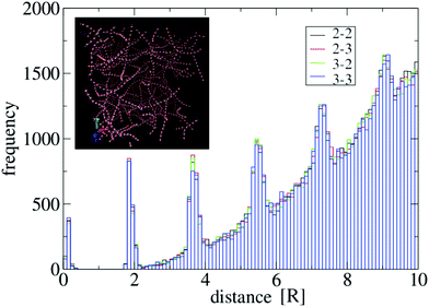 | ||
| Fig. 8 Distribution of distances between sticky spots for a system of N = 2000 particles with λ = 1.75, A = 40ε and σ = 0.4R. Particles are prepared in a homogeneous state and evolved at T = 1 according to eqn (4) in a cubic box with side equal to 54R and periodic boundary conditions. The histogram is representative of the configuration obtained at t = 105τ, see the inset. Black, red, green and blue bars refer respectively to the combination of indices (α,β) = {(2,2),(2,3),(3,2),(3,3)} in the set of distances djβiα for i, j = 1,…,N. Their distributions overlap very well, as expected from symmetry reasons. Multiple peaks above the gap region derive from the regular spacing of particles in the strands. | ||
Simulations have been performed for a system of N = 3 interacting particles confined in a spherical volume with radius R0 = 10.85R and volume fraction ϕ ≃ 2 × 10⁻³, which corresponds to the value of particle density of large-scale simulations with N = 2000. We have verified that in this minimal setup the confining volume is sufficiently larger than the typical particle volume, so that it does not introduce significant finite-size effects. The free energy difference ΔF32 is computed via the equilibrium Boltzmann distribution ΔF32 = −T![[thin space (1/6-em)]](https://www.rsc.org/images/entities/char_2009.gif) log(P3/P2), where P3 and P2 are respectively the occupation probabilities of states “3” and “2” sampled over the equilibrium Brownian dynamics. Parallel tempering evolution is performed for a total time of 5 × 10⁶τ with a swapping period of 50τ. Temperature swaps are realized between adjacent temperature states within the set of temperatures considered in Fig. 3(a).
log(P3/P2), where P3 and P2 are respectively the occupation probabilities of states “3” and “2” sampled over the equilibrium Brownian dynamics. Parallel tempering evolution is performed for a total time of 5 × 10⁶τ with a swapping period of 50τ. Temperature swaps are realized between adjacent temperature states within the set of temperatures considered in Fig. 3(a).
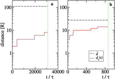
![[d with combining macron]](https://www.rsc.org/images/entities/i_char_0064_0304.gif) = ρnum−1/3 with the typical size dc(t) of the biggest cluster of particles found in the system at time t. We define dc(t) = 2RNc(t), where Nc(t) is the total number of particles in the cluster. We focus on two sizes, namely N = 25 (Fig. 9(a)) and N = 1600 (Fig. 9(b)), which belong respectively to the diffusive and ballistic condensation regime. For N = 25 we find
= ρnum−1/3 with the typical size dc(t) of the biggest cluster of particles found in the system at time t. We define dc(t) = 2RNc(t), where Nc(t) is the total number of particles in the cluster. We focus on two sizes, namely N = 25 (Fig. 9(a)) and N = 1600 (Fig. 9(b)), which belong respectively to the diffusive and ballistic condensation regime. For N = 25 we find ![[d with combining macron]](https://www.rsc.org/images/entities/i_char_0064_0304.gif) ≫ dc(t) during the whole period in which f0 > f* while the case N = 1600 displays a quick growth of dc(t) to values which are of the same order of
≫ dc(t) during the whole period in which f0 > f* while the case N = 1600 displays a quick growth of dc(t) to values which are of the same order of ![[d with combining macron]](https://www.rsc.org/images/entities/i_char_0064_0304.gif) thus suppressing the diffusive scaling of t0.45
thus suppressing the diffusive scaling of t0.45
Acknowledgements
We thank Alberto Rosso and Riccardo Sanson for useful discussions. We acknowledge support from Progetto di Ricerca Dipartimentale BIRD173122/17 of the University of Padova. Part of our simulations were performed in the CloudVeneto platform.Notes and references
- R. G. Weiss and P. Terech, Molecular Gels, Springer, Nederlands, 2006 Search PubMed.
- M. Jehser and C. N. Likos, Colloid Polym. Sci., 2020, 1–11 Search PubMed.
- M. E. Cates and S. M. Fielding, Adv. Phys., 2006, 55, 799–879 CrossRef CAS.
- R. G. Larson, The structure and rheology of complex fluids, Oxford Univesity Press, New York, 1999 Search PubMed.
- J. R. Gomez-Solano and C. Bechinger, New J. Phys., 2015, 17, 103032 CrossRef.
- J. Berner, B. Müller, J. R. Gomez-Solano, M. Krüger and C. Bechinger, Nat. Commun., 2018, 9, 999 CrossRef.
- M. S. Turner and M. E. Cates, J. Phys., 1990, 51, 307–316 CrossRef.
- T. J. Drye and M. E. Cates, J. Chem. Phys., 1992, 96, 1367 CrossRef CAS.
- R. Granek and M. E. Cates, J. Chem. Phys., 1992, 96, 4758 CrossRef CAS.
- M. S. Turner, C. Marques and M. E. Cates, Langmuir, 1993, 9, 695–701 CrossRef CAS.
- J. M. Dealy, Rheol. Bull., 2010, 79, 14–18 Search PubMed.
- R. J. Poole, Rheol. Bull., 2012, 53, 32–39 Search PubMed.
- J. T. Padding, E. S. Boek and W. J. Briels, J. Phys.: Condens. Matter, 2005, 17, S3347–S3353 CrossRef CAS.
- J. T. Padding, E. S. Boek and W. J. Briels, J. Chem. Phys., 2008, 129, 074903 CrossRef CAS.
- V. Hugouvieux, M. A. V. Axelos and M. Kolb, Soft Matter, 2011, 7, 2580 RSC.
- S. Dhakal and R. Sureshkumar, J. Chem. Phys., 2015, 143, 024905 CrossRef.
- P. Wang, S. Pei, M. Wang, Y. Yan, X. Sun and J. Zhang, J. Colloid Interface Sci., 2017, 494, 47–53 CrossRef CAS.
- T. Mandal, P. H. Koenig and R. G. Larson, Phys. Rev. Lett., 2018, 121, 038001 CrossRef CAS.
- F. Sciortino, C. De Michele, S. Corezzi, J. Russo, E. Zaccarelli and P. Tartaglia, Soft Matter, 2009, 5, 2571–2575 CAS.
- W. Li, H. Palis, R. Mérindol, J. Majimel, S. Ravaine and E. Duguet, Chem. Soc. Rev., 2020, 49, 1955 RSC.
- D. J. Audus, F. W. Starr and J. F. Douglas, Soft Matter, 2018, 14, 1622–1630 RSC.
- J. Russo, J. Tavares, P. Teixeira, M. T. da Gama and F. Sciortino, Phys. Rev. Lett., 2011, 106, 085703 CrossRef CAS.
- J. Russo, J. Tavares, P. Teixeira, M. T. da Gama and F. Sciortino, J. Chem. Phys., 2011, 135, 034501 CrossRef CAS.
- L. Rovigatti, J. M. Tavares and F. Sciortino, Phys. Rev. Lett., 2013, 111, 168302 CrossRef.
- P. Teixeira and J. Tavares, Curr. Opin. Colloid Interface Sci., 2017, 30, 16–24 CrossRef CAS.
- L. Rovigatti, J. Russo and F. Romano, Eur. Phys. J. E: Soft Matter Biol. Phys., 2018, 41, 59 CrossRef.
- Q. Chen, S. Chul Bae and S. Granick, Nature, 2011, 469, 381 CrossRef CAS.
- F. Romano and F. Sciortino, Soft Matter, 2011, 7, 5799 RSC.
- F. Romano and F. Sciortino, Nat. Mater., 2011, 10, 171 CrossRef CAS.
- F. Romano and F. Sciortino, Nat. Commun., 2012, 3, 975 CrossRef.
- N. A. Mahynski, L. Rovigatti, C. N. Likos and A. Z. Panagiotopoulos, ACS Nano, 2016, 10, 5459–5467 CrossRef CAS.
- W. F. Reinhart and A. Z. Panagiotopoulos, J. Chem. Phys., 2016, 145, 094505 CrossRef.
- H. Eslami, N. Khanjari and F. Mueller-Plathe, J. Chem. Theory Comput., 2019, 15, 1345–1354 CrossRef.
- T. Tlusty and S. Safran, J. Phys.: Condens. Matter, 2000, 12, A253 CrossRef CAS.
- A. Zilman, S. Safran, T. Sottmann and R. Strey, Langmuir, 2004, 20, 2199–2207 CrossRef CAS.
- S. Plimpton, J. Comput. Phys., 1995, 117, 1–19 CrossRef CAS.
- S. Hyde, Z. Blum, T. Landh, S. Lidin, B. Ninham, S. Andersson and K. Larsson, The language of shape: the role of curvature in condensed matter: physics, chemistry and biology, Elsevier, 1996 Search PubMed.
- W. Zou, G. Tan, H. Jiang, K. Vogtt, M. Weaver, P. Koenig, G. Beaucage and R. G. Larson, Soft Matter, 2019, 15, 642–655 RSC.
- R. H. Swendsen and J.-S. Wang, Phys. Rev. Lett., 1986, 57, 2607–2609 CrossRef.
- M. Tesi, E. J. Van Rensburg, E. Orlandini and S. Whittington, J. Stat. Phys., 1996, 82, 155–181 CrossRef.
- K. Vogtt, H. Jiang, G. Beaucage and M. Weaver, Langmuir, 2017, 33, 1872–1880 CrossRef CAS.
- H. Jiang, K. Vogtt, J. B. Thomas, G. Beaucage and A. Mulderig, Langmuir, 2018, 34, 13956–13964 CrossRef CAS.
- S. Chandrasekhar, Rev. Mod. Phys., 1943, 15, 1 CrossRef.
- G. Carnevale, Y. Pomeau and W. Young, Phys. Rev. Lett., 1990, 64, 2913 CrossRef.
- M. S. Veshchunov, J. Aerosol Sci., 2010, 41, 895–910 CrossRef CAS.
- Z. Chu, Y. Feng, H. Sun, Z. Li, X. Song, Y. Han and H. Wang, Soft Matter, 2011, 7, 4485 RSC.
- P. Cordier, F. Tournilhac, C. Soulié-Ziakovic and L. Leibler, Nature, 2008, 451, 977 CrossRef CAS.
- T. F. A. de Greef and E. W. Meijer, Nature, 2008, 453, 171 CrossRef CAS.
- E. Del Gado and W. Kob, Europhys. Lett., 2005, 72, 1032–1038 CrossRef CAS.
- E. Zaccarelli, P. J. Lu, F. Ciulla, D. A. Weitz and F. Sciortino, J. Phys.: Condens. Matter, 2008, 20, 494242 CrossRef.
- R. Angelini, E. Zaccarelli, F. A. de Melo Marques, M. Sztucki, A. Fluerasu, G. Ruocco and B. Ruzicka, Nat. Commun., 2014, 5, 4049 CrossRef CAS.
- C. S. Dias, N. A. M. Araújo and M. M. T. da Gama, Adv. Colloid Interface Sci., 2017, 247, 258–263 CrossRef CAS.
- N. G. Almarza, Phys. Rev. E: Stat., Nonlinear, Soft Matter Phys., 2012, 86, 030101 CrossRef CAS.
| This journal is © The Royal Society of Chemistry 2020 |

