DOI:
10.1039/D0SM01113D
(Paper)
Soft Matter, 2020,
16, 10358-10367
Thermal shape fluctuations of a two-dimensional compressible droplet
Received
16th June 2020
, Accepted 8th September 2020
First published on 10th September 2020
Abstract
Analysis of thermal capillary waves on the surface of a liquid usually assumes incompressibility of the bulk fluid. However, for droplets or bubbles with submicronic size, or for epithelial cells whose out-of-plane elongation can be modeled by an effective 2D bulk modulus, compressibility of the internal fluid must be taken into account for the characterization of their shape fluctuations. We present a theoretical analysis of the fluctuations of a two-dimensional compressible droplet. Analytical expressions for area, perimeter and energy fluctuations are derived and compared with Cellular Potts Model (CPM) simulations. This comparison shows a very good agreement between theory and simulations, and offers a precise calibration method for CPM simulations.
Thermal capillary waves have been the subject of intense research activity, both theoretically and experimentally,1–3 and their experimental characterization allows for a precise measurement of surface tension.4 In the case of fluctuating closed surface, as for a droplet, a bubble or a vesicle, it is usually assumed that the internal fluid is incompressible.5–7 This constraint is handled by expressing the fundamental mode of fluctuations in terms of higher modes. The relative importance of surface and compression energies is determined by the dimensionless parameter ε = γ/(Br0), where γ is the surface tension, B the bulk modulus, and r0 the radius of the droplet. For common liquids, γ ∼ 10−3–10−2 N m−1 and B ∼ 105 Pa, so the incompressibility approximation is absolutely justified for droplet size larger than ∼1 μm. For droplet with submicronic size however, finite compressibility should be taken into account to properly reflect their fluctuation spectrum. Effect of compressibility is also relevant for the study of biological cell conformation in a monolayer, despite their supermicronic size: when analyzing the contour fluctuations of their apical surface, their out-of-plane elongation can be modeled by an effective two-dimensional (2D) bulk modulus.8 This effective 2D compressibility is taken into account in most numerical modelling of cell monolayers,9–12 in addition to their bending and/or stretching energy.
With this aim in mind, we investigate in this paper the thermal fluctuations of a “two-dimensional” compressible droplet with low (but finite) compressibility; this may correspond to a droplet squeezed between two parallel plates. Analytical expressions for the average and variance of area, perimeter and energy are derived and compared with Cellular Potts Model (CPM) simulations, which is a standard numerical modelling of soft cellular systems. The present article is organized as follows. In Section 1, we evaluate the partition function of a 2D droplet with low but finite compressibility. The calculations are more complicated than in the incompressible case because the compressing energy introduces quartic terms of the contour position vector which cannot be neglected. In Sections 2 and 3 we derive analytical expressions for the average and standard deviations of the area, contour length, and energy, which fully characterize their normal probability distributions. In Section 4 we calculate the mean square amplitude of the contour fluctuation modes. Then, in Section 5 we confront the different expressions with numerical simulations performed with CPM simulations. The agreement between theory and numerical data is very good, and offers a robust method for calibrating surface tension in CPM. In particular, we explain in Section 6 that we are able to detect a slight thermal softening of CPM surface tension which is caused by shorter wavelength modes.
1 Partition function and free energy
Let us consider a two-dimensional droplet surrounded by a fluid with uniform pressure P0 and temperature T. We assume that a droplet configuration is entirely determined by its shape. Such a description is valid as long as the equilibration of molecules in the bulk and along the boundary is fast in comparison to the typical velocity of the droplet boundary. Then, its energy has two contributions (see Appendix A for their derivation from a microscopic description):The first contribution is the boundary energy: ![[script letter H]](https://www.rsc.org/images/entities/char_e142.gif) b = γL, where γ is the line tension (i.e. surface tension times the transverse height), and
b = γL, where γ is the line tension (i.e. surface tension times the transverse height), and  is the (fluctuating) contour length. The second contribution is the bulk compressive energy:
| |  | (2) |
where B is the 2D bulk modulus of the internal fluid, measured at atmospheric pressure P0, A the fluctuating area of the droplet, and A0 its nominal area (the area that the internal fluid occupies when the inner pressure matches P0).
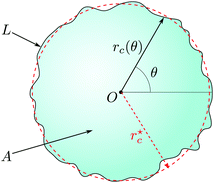
To describe the vesicle contour, it is convenient to use the polar parametrization θ ↦ rc(θ), as shown in Fig. 1, where the location of the center O is chosen arbitrarily for the moment. The perimeter and area of the droplet can be expressed as functionals of rc(θ):
| |  | (3) |
 |
| | Fig. 1 Thermal fluctuations of a two-dimensional droplet. | |
The relative importance of boundary, compression, and thermal energies are characterized by two dimensionless quantities: the relative compressibility ε = γ/Br0 already introduced above, and the relative amplitude of fluctuations η = kBT/γr0, where  . We consider here the low compressibility (ε ≪ 1) and low fluctuations (η ≪ 1) regime. In order to derive an analytical expression for the partition function, we need to expand the Hamiltonian around a reference configuration that we determine below.
1.1 Reference configuration
The most obvious choice of reference conformation is the one that minimizes the droplet energy. Given the isotropy of the problem, we can already affirm that this conformation of the 2D compressible drop will be a disk. Therefore, if we choose the origin O at the center of mass of the droplet, the function rc(θ) that minimizes ![[script letter H]](https://www.rsc.org/images/entities/char_e142.gif) [rc(θ)] is a constant r⋆. Minimization of the Hamiltonian with respect to rc(θ) leads to
[rc(θ)] is a constant r⋆. Minimization of the Hamiltonian with respect to rc(θ) leads to| |  | (4) |
where A⋆ = A[r⋆] = πr⋆2. Eqn (4) is just the Laplace's law, the first term being equal to the pressure difference P0 − P⋆. This equation implicitly determines r⋆. Introducing the dimensionless radius ![[r with combining tilde]](https://www.rsc.org/images/entities/i_char_0072_0303.gif) = r⋆/r0, eqn (4) rewrites:
= r⋆/r0, eqn (4) rewrites:| | ![[r with combining tilde]](https://www.rsc.org/images/entities/i_char_0072_0303.gif) 3 − 3 − ![[r with combining tilde]](https://www.rsc.org/images/entities/i_char_0072_0303.gif) + ε = 0. + ε = 0. | (5) |
This cubic equation has positive roots only if  , which then defines the stability criterion for the circular droplet: when ε > εc, the droplet collapses. When ε < εc, there are two positive roots which correspond to a maximum and a minimum of the energy, respectively. The latter corresponds to the stable configuration, and expresses as:
| |  | (6) |
Expansion of the right-hand-side term in the low compressibility regime yields:
| |  | (7) |
1.2 Expansion of ![[script letter H]](https://www.rsc.org/images/entities/h3_char_e142.gif)
Let us introduce u(θ), the dimensionless displacement of the contour relatively to its reference configuration: rc(θ) = r⋆(1 + u(θ)). Expansion of L and A (eqn (3)) up to second order in u and u′ yields:| |  | (8) |
and| |  | (9) |
It is useful for the rest to express theses quantities in terms of the Fourier coefficients {ũp}, defined as:| |  | (10) |
where N ≫ 1 is the number of (coarse-grained) points that define the boundary location. The distance between consecutive points in the reference configuration is then a = L⋆/N (typically, a is equal to a few molecular sizes). The variables {ũℜp,ũℑp;0 ≤ p ≤ N/2} (where ũℜp = Re(ũp), ũℑp = Im(ũp), and ũℑ0 = ũℑN/2 = 0) constitute a set of N independent real variables. The perimeter and area then express as:| |  | (11) |
| |  | (12) |
where L⋆ = 2πr⋆ is the perimeter of the reference configuration. Finally, the partition function reads:| |  | (13) |
where L and A are given by eqn (11) and (12), and β = 1/kBT. The integration measure reads| |  | (14) |
where the quantum of height fluctuation λ has been introduced to make the measure dimensionless. Note that we omitted the Jacobian associated with the change from real to Fourier space variables: since this is a linear change of variables, the Jacobian is uniform and depends only on N. We also omitted the two real modes p = 1 in the measure, which correspond to independent global translations of the droplet within the plane: their values have been set to zero by fixing the frame origin O onto the droplet's center of mass.
The Hamiltonian rewrites:
| |  | (15) |
In the incompressible case, the Gaussian approximation consists in expanding the boundary term up to second order in |
ũp|. Then, the mean quadratic amplitude of fluctuations is found to scale linearly with
η in the small fluctuations regime: 〈|
ũp|〉
2 ∼
η.
13 Here, because of the prefactor
ε in the boundary term, the compressibility term must be expanded up to fourth order in |
ũp| while expanding the boundary term up to second order. The presence of quartic terms
![[scr O, script letter O]](https://www.rsc.org/images/entities/char_e52e.gif)
(|
ũp|
4) in the Hamiltonian makes the evaluation of
Z more difficult than in the incompressible case. One way to tackle this problem is by using the Hubbard–Stratonovich transformation to linearize the (
A −
A0)
2 term in
eqn (13). This method is developed in Appendix B. Here we choose another method, which consists in making the change of variables
ũ0,{
ũp≥2} →
A,{
ũp≥2} in order to express
Z as Gaussian integrals. The fact that the two methods give the same expression for
Z increases our confidence in the final result. We express
ũ0 in terms of the new set of variables by solving the second order
eqn (12). Assuming low compressibility and small fluctuations (|
A −
A⋆|/
A⋆ ≪ 1, |
ũp≥2| ≪ 1), the only physical root simplifies to:
| |  | (16) |
The next term in the expansion,
![[scr O, script letter O]](https://www.rsc.org/images/entities/char_e52e.gif)
(((
A −
A⋆)/
A⋆)
2), has a negligible contribution to the Hamiltonian in comparison with the compression term

. Inserting
eqn (16) into
eqn (11), we finally obtain the expression of
![[script letter H]](https://www.rsc.org/images/entities/char_e142.gif)
in terms of the new set of variables:
| |  | (17) |
Hence, the partition function rewrites in terms of the new set of variables as:
| |  | (18) |
where |ℑ| is the Jacobian associated with the change of variables, and
| |  | (19) |
We show in Appendix C that |ℑ| = 1/(2
A⋆). Integrating over variables {
ũℜp,
ũℑp;
p ≥ 2}, we get:
| | 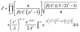 | (20) |
Strictly, the integral over
A is ranged on all positive real areas. But the integrand is a Gaussian function centered in the vicinity of
A0, with a spread of order

. One can then expand the range of the integral to the real axis, yielding:
| | 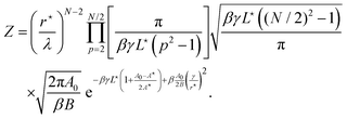 | (21) |
Finally, the free energy of the droplet
F = −
kBT![[thin space (1/6-em)]](https://www.rsc.org/images/entities/char_2009.gif)
ln
![[thin space (1/6-em)]](https://www.rsc.org/images/entities/char_2009.gif) Z
Z has for expression (up to additive constants):
| |  | (22) |
2 Statistics over perimeter and area
We can now determine the statistical distribution of the geometrical variables A and L. According to eqn (17) and (18), the area probability distribution is P(A) ∝ e−f(A), with| |  | (23) |
Hence, the area probability distribution follows a Gaussian law whose mean value 〈A〉 and variance (ΔA)2 are given by f′(〈A〉) = 0 and (ΔA)2 = 1/f′′(〈A〉), respectively. The first equation gives| |  | (24) |
where the last equality has been deduced from eqn (4); the average area then coincides with the area of the minimal energy configuration. The second equation gives:| |  | (25) |
Expressing the Hamiltonian (eqn (17)) in terms of the variables L,{ũp≥1} instead, one finds that the perimeter droplet also follows a Gaussian distribution: P(L) ∼ e−(L−L)2/(2ΔL2). The average perimeter can be easily expressed using the identity  (considering A⋆, L⋆, r⋆ as constants). It comes:
| |  | (26) |
Using
eqn (4), the two last terms cancel each other and we end up with:
| |  | (27) |
Similarly, statistical variance of the perimeter is obtained using (Δ
L)
2 = −
kBT∂
2F/∂
γ2:
| |  | (28) |
3 Statistics over energy
We now characterize the fluctuations of the energy, which is of primary physical importance. The probability distribution of energy follows the Boltzmann statistics:where g(E) is the density of states of energy E. Using eqn (17) and (4), the energy expresses as:| |  | (30) |
where E⋆ is the energy of the reference configuration. The density g(E) can then be easily determined by noticing that the hypersurface of constant energy is an ellipsoid in the space of the variables A − 〈A〉,{ũp≥2}. It can be transformed into a hypersphere with radius  in the space of variables Xi (1 ≤ i ≤ N − 2), with:
  ,
,  for 1 ≤ k ≤ N/2 − 1, and
  for 1 ≤ k ≤ N/2 − 2. The volume occupied by one state remains uniform through this linear change of variables. Therefore,where d = N − 2 is the space dimension and Ωd = 2πd/2/Γ(d/2) is the surface of a d-sphere with unit radius; Γ is the Euler Gamma function. For N ≫ 1, we then have g(E) ∼ (E − E⋆)N/2, and thus
| | | P(E) = c(E − E⋆)N/2e−βE, | (32) |
where the constant c is determined through normalization. This distribution is peaked around its more probable configuration. We can then approximate its expression with a normal distribution using Laplace's method: P(E) = ceh(E) ∼ e−(E−〈E〉)/(2(ΔE)2) where 〈E〉 and (ΔE)2 are determined from h′(〈E〉) = 0 and (ΔE)2 = −1/h′′(〈E〉). It comes:| |  | (33) |
and| |  | (34) |
4 Statistics over mode amplitudes
The last analytical expressions we derive are for the average and variance of mode amplitudes ũp. According to the Hamiltonian expression (eqn (17)), fluctuations of ũℜp and ũℑp (with p ≥ 2) follow normal distributions. We deduce immediately:| |  | (35) |
| |  | (36) |
Finally, the mean amplitude of mode p = 0, which corresponds to a uniform compression of the droplet, is obtained from eqn (16): as 〈A〉 = A⋆ (eqn (24)), and using the mathematical identity  , it comes:
| |  | (37) |
We stress out that 〈
u〉 = 〈
ũ0〉 ≠ 0: the average radius value
rc (also equal to its more likely value) does not coincide with its zero temperature value
r⋆. The second moment 〈
ũ02〉 is an infinitesimal term of higher order which cannot be captured by our approach. Note that the effect of finite compressibility in
eqn (35)–(37) is wholly contained in
L⋆.
5 Numerical simulations
In this section we compare our analytical predictions with numerical simulations made with the Cellular Potts Model (CPM). The benefit of this comparison is twofold: first, the accuracy of our expressions can be tested by varying the different input parameters. Second, it offers an original method to calibrate CPM simulations for which surface tension is defined up to a prefactor whose value depends on the range of interactions used in simulations.14 This will be particularly helpful for future extension of this work to multicellular systems.
5.1 Cellular Potts model
Cellular Potts model is a 2D lattice-based model (usually a square lattice) which is widely used for simulating cellular systems in various fields of physics or biology.9,12,15–18 Each cell is represented as a subset of lattice sites sharing the same cell ID (analogical to spins in Potts model). Cellular domains can adopt any shape on the lattice. The CPM is then particularly suited to simulate thermal fluctuations of cellular systems, as it reproduces realistically the fluctuations of interface locations, even for wavelength at subcellular scale. Furthermore, its extension to three dimensions is straightforward.
The boundary energy term in CPM simulations is defined as:
| |  | (38) |
The second sum is carried over all sites
l that are in the coupling neighborhood of site
k,
![[scr N, script letter N]](https://www.rsc.org/images/entities/char_e52d.gif) c
c(
k), and
σk,
σl are the cell IDs of site
k and
l, respectively.
δ is the Kronecker delta symbol:
δm,n = 1 if
m =
n, and 0 otherwise. The coupling constant
J > 0 sets the amplitude of surface tension. As the range of the coupling neighborhood increases, the estimation of contact energy is smoother and gradually erases the square lattice anisotropy. However, we show below that this also generates a slight dependence of the effective surface tension with simulation temperature.
Definition of length on lattice-based models such as CPM must be done cautiously, as it is a common source of confusion and implementation errors.19 Here we define the length of the boundary from its energy. We consider that site k belongs to the boundary as soon as there is a site in its coupling neighborhood whose label is different from σk. Therefore, a boundary in CPM has a thickness which is directly related to the size of coupling neighborhood. Let us introduce z, the number of sites with ID ≠ σk in the coupling neighborhood of a boundary site k, averaged over all sites k that belong to that boundary. We then define the boundary length as  , i.e. the boundary energy measured for a unit coupling constant, divided by the boundary thickness z. Accordingly, surface tension is given by γ = zJ (in units of energy per pixel2). Roughly, z is equal to half of the number of sites in the coupling neighborhood. Actually, because of the anisotropy of the underlying lattice, z – and so γ – slightly depend on the contour shape: their values will be different for a square and a circular contour. Values of z reported in the literature range from 10.5 to 11.319–21 for 4th order coupling neighborhood, which has 20 neighboring lattice sites (see Fig. 2). Here we propose to take advantage of the thermal fluctuations of the contour and perform statistical averaging to lessen this dependency on contour shape, and determine an accurate value for z.
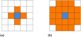 |
| | Fig. 2 (a) Order I neighborhood, with 4 lattice sites (in orange), is used as target neighborhood in our simulations, in which the target value is chosen from in the updating rule. (b) Order IV neighborhood, with 20 lattice sites (in orange), is used as coupling neighborhood ![[scr N, script letter N]](https://www.rsc.org/images/entities/char_e52d.gif) c for computing the boundary energy (eqn (38)). c for computing the boundary energy (eqn (38)). | |
5.2 Results
To ensure accuracy of the results, simulations were performed in duplicate with an home-made software and the CompuCell3D software (CC3D).22 The former uses a recently modified Metropolis algorithm that preserves the integrity of the cellular domains and satisfies the detailed balance equation,14 ensuring that the probability distribution of visited states converges to the Boltzmann distribution.12,14 Recent versions of the latter incorporate the non-fragmentation part of our algorithm.14 However, we also had to modify the updating rule in the CC3D core in order to fully restore the detailed balance equation, in agreement with ref. 14. Without these modifications, we observed a significant departure from both the home-made software simulations and analytical predictions. These modifications are detailed in the Appendix D.
The coupling neighborhood ![[scr N, script letter N]](https://www.rsc.org/images/entities/char_e52d.gif) c, used for calculation of the boundary energy is the order IV neighborhood, with 20 neighbors for each pixel. The target neighborhood, in which the target value is chosen from in the site updating rule of the Metropolis-like algorithm, is the order I neighborhood, with 4 neighbors per pixel (see Fig. 2).
c, used for calculation of the boundary energy is the order IV neighborhood, with 20 neighbors for each pixel. The target neighborhood, in which the target value is chosen from in the site updating rule of the Metropolis-like algorithm, is the order I neighborhood, with 4 neighbors per pixel (see Fig. 2).
We run simulations for different points in the phase space {J,B,T,A0}, in a way that the two dimensionless parameters ε and η are varied independently. We ensure that values of variables are in ranges such that the hypotheses we made in our theoretical model stay valid in simulations. Namely, we ensured weak bulk compressibility (ε ≤ 0.1), small thermal fluctuations (η ≤ 0.1), and a sufficient number of degrees of freedom for the membrane (a/r0 ≪ 1), where here a and z are taken to be of order 1 and 10 pixels, respectively. Each simulation was run for 106 Monte-Carlo steps, and statistics are performed over 2 × 10⁻⁴ measures. The number of uncorrelated samples is obtained using the pymbar.timeseries module,23 so that uncertainties of the measured quantities are based on fully independent samples.
We want to use the comparison with theory to determine the values of the two unknown parameters z and a. We then introduce the uncalibrated/raw length L′ = ![[script letter H]](https://www.rsc.org/images/entities/char_e142.gif) b/J, the calibrated length being L = L′/z, and we rewrite eqn (24), (25), (27), (28), (33) and (34) in terms of the dimensionless variables ε′ = J/Br0 and η′ = kBT/Jr0, rather than ε = zε′, η = η′/z. Using expansion eqn (7) for r⋆, we obtain:
b/J, the calibrated length being L = L′/z, and we rewrite eqn (24), (25), (27), (28), (33) and (34) in terms of the dimensionless variables ε′ = J/Br0 and η′ = kBT/Jr0, rather than ε = zε′, η = η′/z. Using expansion eqn (7) for r⋆, we obtain:
| |  | (39) |
| |  | (40) |
| |  | (41) |
| |  | (42) |
| |  | (43) |
| |  | (44) |
where

. It can be noticed that the distribution of area, perimeter and energy are all affected by the finite compressibility of the droplet.
Fig. 3 shows the typical histograms of A, L′ and E obtained for one simulation run. In agreement with our theoretical treatment, they all follow Gaussian distributions. We then report the variation of different quantities as function of the dimensionless variables ε′ and η′, and use expressions eqn (39)–(44) as fitting functions, where a and z are the two adjusting parameters. Fit values of z and a are summarized in Fig. 4.
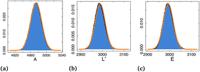 |
| | Fig. 3 Histograms of perimeter L, area A and energy E. Orange curve are Gaussian functions whose mean and variance are calculated from the corresponding histogram. | |
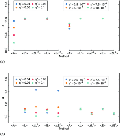 |
| | Fig. 4 Fit values for z and a obtained using expressions (39)–(44) with numerical data. Values reported with open symbols were obtained by setting the value of either z or a and using only the other one as a fitting parameter. | |
Fig. 5 shows the variation of 〈A〉/A0 and (ΔA/A0)2 with ε′ and η′. In agreement with eqn (39), we observe in Fig. 5a clear linear dependence of 〈A〉/A0 on ε′ whose slope provides a first estimation for z. However, we observe a slight dependence of the slope on η′, which is not predicted by eqn (39). This suggests that the CPM calibration parameter z slightly decreases as η′ increases. This weak dependence can also be observed in Fig. 5b: a linear fit of the data for a given ε′ value yields a small positive slope, indicating that z – and hence, the surface tension in CPM simulations – is a slightly decreasing function of η′. We discuss in Section 6 of the origin of this thermal softening of surface tension. Expression of the area variance (eqn (40)) does not depend on z and a, and the comparison with numerics in Fig. 5c and d is done with no adjusting parameter. Nevertheless, the agreement is very good.
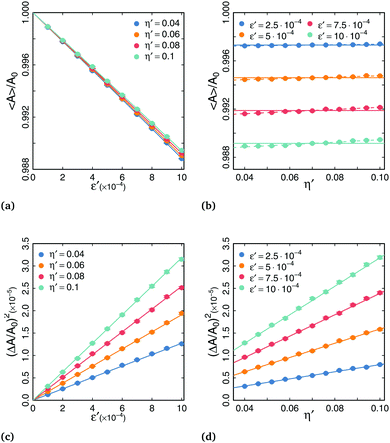 |
| | Fig. 5 (a) Variation of 〈A〉/A0 with dimensionless parameter ε′. Solid curves are fits using eqn (39) with adjusting parameter z. (b) Variation of 〈A〉/A0 with dimensionless parameter η′. Solid curves are averages. Dashed curves are linear fits. (c and d) Variation of (ΔA/A0)2 with dimensionless parameters ε′ and η′. Solid curves correspond to eqn (40) with no adjusting parameters. | |
Fig. 6 shows the variation of 〈L′〉/L0 and (ΔL/L0)2 with ε′ and η′. Fits are in excellent agreement with eqn (41) and (42), giving credence to our theoretical treatment. For the variation of 〈L〉/L0 with η′, z derived from the fits are in the expected range. Values are slightly above those deduced from the mean area, because the decrease of the proportionality coefficient between γ and J at short wavelength has different impact on the coarse-grained curvature and perimeter of the droplet. Fits in Fig. 6a, c, and d do not allow to determine precisely both z and a, as a whole range of pairs of parameter values gives similar data fit. For these curves, the value of z was set to the one obtained from fitting the variation of 〈L〉/L0 with η′, and a was left as the only adjusting parameter. Values obtained for a from are in a narrow range (a ∼ 1.1), and in agreement with our expectation: a step of a = 1 pixel corresponds to a boundary aligned with one of the square lattice axes. The fact that values are slightly above 1 can be attributed to the finite curvature 1/r⋆ of the droplet, and to the contribution of other boundary orientations in the averaging. Values of a obtained from the variation of (ΔL/L0)2 with ε′ show a slight dependence with η′, and are more spread out than other values. This dependence can be explained from the variation of z with η′ revealed earlier, which has been ignored in the fits, as they were performed with the same value for z.
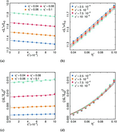 |
| | Fig. 6 (a and b) Variation of 〈L〉/L0 with dimensionless parameters ε′ and η′. Solid curves are fits using eqn (41) with adjusting parameters z and a. (c and d) Variation of (ΔL/L0)2 with dimensionless parameters ε′ and η′. Solid curves correspond to eqn (42) with adjusting parameter a. | |
We now test our predictions on statistical distribution of energy (eqn (43) and (44)). Variations of 〈E〉/JL0 and (ΔE/JL0)2 are shown in Fig. 7. Again, we have perfect agreement between the numerical data and the fits from the analytical expressions. The values for z and a obtained from these fits are almost identical to the ones obtained from the statistical distribution of perimeter. The energy is a function of perimeter and surface area, and since the boundary energy is much larger than the bulk compressive energy, it comes as no surprise that we observe similar trends for the energy and the perimeter.
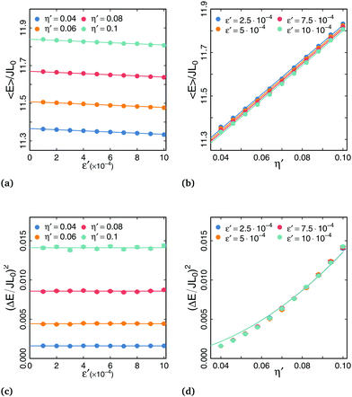 |
| | Fig. 7 (a and b) Variation of 〈E〉/JL0 with dimensionless parameters ε′ and η′. Solid curves are fits using eqn (43) with adjusting parameter z and a. (c and d) Variation of (ΔE/JL0)2 with dimensionless parameters ε′ and η′. Solid curves correspond to eqn (44) with adjusting parameter a. | |
Finally, we test our predictions on the amplitudes of modes (eqn (35) and (37)). From the positions rc(θ) of lattice sites localized at the droplet boundary for a given configuration, we deduce u(θ) = rc(θ)/r⋆ − 1, where  , and then evaluate ũp from eqn (10). Fig. 8 shows the variation of 〈|ũp2|〉 with p. Again, data are well predicted by the theoretical expression eqn (35), and yields for the unique fit parameter z = 10.88, consistent with values obtained from other expressions (see Fig. 4). We also reported on the graph −4〈ũ0〉/9 calculated with this value of z. In agreement with eqn (37), its value is very close to 〈|ũ2|〉2.
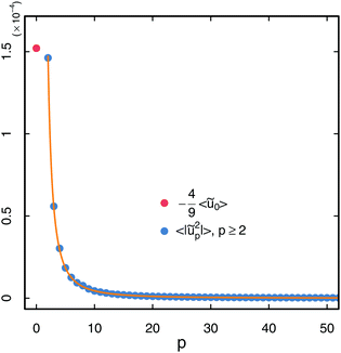 |
| | Fig. 8 Mean square amplitude of fluctuation modes ũp. Orange curve is a fit using eqn (35) with z as adjusting parameter. Fit value is z = 10.88. The simulation was done with parameters A0 = 5000, ε′ = 3 × 10⁻⁴, and η′ = 0.03. | |
6 Discussion
The remarkable agreement between the numerical data and the fits from the analytical expressions validates our theoretical treatment. Note that as our analytical expressions are based on expansions in the dimensionless parameters ε and η, we expect the relative error with exact theory to be ![[scr O, script letter O]](https://www.rsc.org/images/entities/char_e52e.gif) (ε,η). Values of z and a excerpt from the different fits are consistent with each other. However, we noticed a small decay of z – and hence the CPM surface tension – with the amplitude of thermal fluctuations. We suspect that this thermal softening of surface tension is caused by the short wavelength fluctuating modes: for modes whose wavelength is shorter than the range of interactions between lattice sites (set by the size of coupling neighborhood), the number of unlike lattice sites in the coupling neighborhood of a given site at the boundary is smaller than the one expected for a flat interface. To test this hypothesis, we calculated z explicitly for static configurations of a droplet with modulated radius rc(θ) = r⋆(1 + 0.025
(ε,η). Values of z and a excerpt from the different fits are consistent with each other. However, we noticed a small decay of z – and hence the CPM surface tension – with the amplitude of thermal fluctuations. We suspect that this thermal softening of surface tension is caused by the short wavelength fluctuating modes: for modes whose wavelength is shorter than the range of interactions between lattice sites (set by the size of coupling neighborhood), the number of unlike lattice sites in the coupling neighborhood of a given site at the boundary is smaller than the one expected for a flat interface. To test this hypothesis, we calculated z explicitly for static configurations of a droplet with modulated radius rc(θ) = r⋆(1 + 0.025![[thin space (1/6-em)]](https://www.rsc.org/images/entities/char_2009.gif) cos(2πr⋆θ/λ)) and discretized on a square lattice, with r⋆ = 30 pixels, for varying wavelength λ. Results are shown in Fig. 9: for modes with λ ≳ 10 pixels, z does not really depart from a constant value ≃11.3. For modes with shorter wavelengths, z decreases monotonically down to 10.5. It can be noticed that this range of z values coincides with the range of values reported in literature. This thermal softening effect could then rationalize the scattered values of z found in literature. Moreover, as the thermal softening of the CPM surface tension is caused by the fluctuating modes with wavelength comparable or shorter than the range of lattice site interactions, we expect this effect to be more pronounced when the coupling neighborhood is increased. Hence, the choice for its size should be the result of a trade-off between reducing anisotropy and limiting this unexpected temperature dependence. Presumably this dependence is enhanced in our version of the algorithm that satisfies detailed balance (see Appendix D): consider a rugosity of one single site, on an otherwise flat interface. This site is surrounded by three sites in its target neighborhood having dissimilar labels, and a single one that shares the same label. In the original algorithm, the unlike label is three times more likely to be chosen as the target label than the similar one, whereas they have equal probabilities in the modified version. The rugosity is therefore more likely to be smoothed out in the unmodified version. As rugosities with short wavelengths are the leading cause of thermal softening, this effect is less pronounced when interfaces are flattened.
cos(2πr⋆θ/λ)) and discretized on a square lattice, with r⋆ = 30 pixels, for varying wavelength λ. Results are shown in Fig. 9: for modes with λ ≳ 10 pixels, z does not really depart from a constant value ≃11.3. For modes with shorter wavelengths, z decreases monotonically down to 10.5. It can be noticed that this range of z values coincides with the range of values reported in literature. This thermal softening effect could then rationalize the scattered values of z found in literature. Moreover, as the thermal softening of the CPM surface tension is caused by the fluctuating modes with wavelength comparable or shorter than the range of lattice site interactions, we expect this effect to be more pronounced when the coupling neighborhood is increased. Hence, the choice for its size should be the result of a trade-off between reducing anisotropy and limiting this unexpected temperature dependence. Presumably this dependence is enhanced in our version of the algorithm that satisfies detailed balance (see Appendix D): consider a rugosity of one single site, on an otherwise flat interface. This site is surrounded by three sites in its target neighborhood having dissimilar labels, and a single one that shares the same label. In the original algorithm, the unlike label is three times more likely to be chosen as the target label than the similar one, whereas they have equal probabilities in the modified version. The rugosity is therefore more likely to be smoothed out in the unmodified version. As rugosities with short wavelengths are the leading cause of thermal softening, this effect is less pronounced when interfaces are flattened.
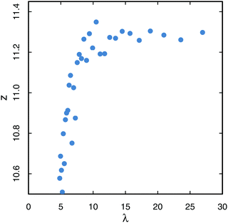 |
| | Fig. 9 Value of z calculated explicitly for static configurations of a droplet drawn on a square lattice, with modulated radius rc(θ) = r⋆(1 + 0.025![[thin space (1/6-em)]](https://www.rsc.org/images/entities/char_2009.gif) cos(2πr⋆θ/λ)) as a function of wavelength λ. cos(2πr⋆θ/λ)) as a function of wavelength λ. | |
7 Conclusion and perspectives
To summarize, we theoretically investigated in this paper the thermal fluctuations of a compressible, two-dimensional droplet in the low compressibility (ε ≪ 1) and small fluctuations (η ≪ 1) regime. This study is relevant for submicronic-sized drops or bubbles, or as a first step towards the more complex case of vesicles or epithelial cells. We hope our results will stimulate experimental work, as our analysis offers a non-invasing tool to probe the mechanical properties (B and γ) of a compressible droplet from the simple measurement of its perimeter and area fluctuations. The different analytical expressions that we derived have been successfully compared with cellular Potts model simulations. Moreover, the comparison between theory and simulations offers a robust calibration method for the cellular Potts model, for which lengths and surface tension are defined up to a multiplicative prefactor. The accuracy of our analytical treatment and numerical simulations reveals a slight dependence of this prefactor with the simulation temperature, previously unseen.
In future extensions to this work, we will consider the case of compressible vesicles by including bending and stretching terms to the boundary energy. We will also extend our analysis to multicellular systems, for which contour fluctuations of every cellular unit are related in a sophisticated way, that involves in particular the topology of the cellular pattern.
Conflicts of interest
There are no conflicts to declare.
Appendix
A Derivation of the coarse-grained Hamiltonian ![[script letter H]](https://www.rsc.org/images/entities/h3_char_e142.gif)
We justify the expression eqn (1) for the Hamiltonian of a two-dimensional droplet surrounded by a fluid with uniform pressure P0 and temperature T, and list the underlying assumptions on which it is based. At the microscopic level, a configuration of the droplet is given by the position rα and momentum pα of every particle α that belongs to the droplet. The coarse-grained Hamiltonian ![[script letter H]](https://www.rsc.org/images/entities/char_e142.gif) [rc(θ)] is defined by gathering all configurations corresponding to a given shape of the droplet, specified by its contour rc(θ):
[rc(θ)] is defined by gathering all configurations corresponding to a given shape of the droplet, specified by its contour rc(θ):| |  | (45) |
Here Hm[{rα,pα}] is the fined-grained Hamiltonian, composed of the kinetic and potential energy of all the molecules. As the interaction range of molecules is much smaller than the droplet size, the contributions to the coarse-grained Hamiltonian can be divided in two parts: a bulk contribution ![[script letter H]](https://www.rsc.org/images/entities/char_e142.gif) c, and a boundary contribution
c, and a boundary contribution ![[script letter H]](https://www.rsc.org/images/entities/char_e142.gif) b. When the thermalization of the inner fluid is much faster than the typical boundary displacements, we can identify
b. When the thermalization of the inner fluid is much faster than the typical boundary displacements, we can identify ![[script letter H]](https://www.rsc.org/images/entities/char_e142.gif) c with the Gibbs free energy of the compressible fluid.
c with the Gibbs free energy of the compressible fluid. ![[script letter H]](https://www.rsc.org/images/entities/char_e142.gif) c then does not depend on the specific shape of the droplet, but on its area A only. The pressure difference between the inner and outer fluids is given by P − P0 = −
c then does not depend on the specific shape of the droplet, but on its area A only. The pressure difference between the inner and outer fluids is given by P − P0 = −![[script letter H]](https://www.rsc.org/images/entities/char_e142.gif) ′c(A)/h, where h is the transverse height of the droplet. Expanding
′c(A)/h, where h is the transverse height of the droplet. Expanding ![[script letter H]](https://www.rsc.org/images/entities/char_e142.gif) c(A) around the nominal value A0, which corresponds to the area value for which P = P0, we get:
c(A) around the nominal value A0, which corresponds to the area value for which P = P0, we get:| |  | (46) |
where B = A0![[script letter H]](https://www.rsc.org/images/entities/char_e142.gif) ′′c(A0) is the 2D bulk modulus of the inner fluid measured at pressure equal to the surrounding pressure (P = P0). Note that the compressive energy is minimal when the inner pressure and area match their outer counterparts. The additive constant
′′c(A0) is the 2D bulk modulus of the inner fluid measured at pressure equal to the surrounding pressure (P = P0). Note that the compressive energy is minimal when the inner pressure and area match their outer counterparts. The additive constant ![[script letter H]](https://www.rsc.org/images/entities/char_e142.gif) c(A0) has been dropped in eqn (2).
c(A0) has been dropped in eqn (2).
The simplest expression for the boundary term reads ![[script letter H]](https://www.rsc.org/images/entities/char_e142.gif) b = γ
b = γ![[script L]](https://www.rsc.org/images/entities/char_e144.gif) ;
; ![[script letter H]](https://www.rsc.org/images/entities/char_e142.gif) b does not depend on the specific shape of the droplet either, but only on its perimeter
b does not depend on the specific shape of the droplet either, but only on its perimeter ![[script L]](https://www.rsc.org/images/entities/char_e144.gif) . Note that this expression implies that surface tension γ is uniform; if the droplet boundary contains surfactant molecules, it is then assumed that fluctuations of their surface concentration can be neglected.
. Note that this expression implies that surface tension γ is uniform; if the droplet boundary contains surfactant molecules, it is then assumed that fluctuations of their surface concentration can be neglected.
B Derivation of Z using Hubbard–Stratonovich transformation
Z can be derived more straightforwardly using Hubbard–Stratonovich transformation:| |  | (47) |
Using this expression with x = A − A0 and a = βB/A0, eqn (13) rewrites| |  | (48) |
Replacing L and A by their expressions (11) and (12), where ũ02 can be neglected in the latter, we obtain:| |  | (49) |
| |  | (50) |
with αp(k) = βγL⋆p2 + i2kA⋆. We can safely switch the integration over k with the integration over ũℜp, ũℑp for p ≥ 2. But because  , it cannot be switched with the integral over ũ0. This peculiarity is specific to the case studied here: it does not arise when adding bending term in the energy,24 or for an initially flat geometry, or even when using fixed boundary conditions rather than periodic ones. To compute Z, we first calculate Z(
![[small script l]](https://www.rsc.org/images/entities/char_e146.gif) ), which is defined identically to Z, except for the integration over ũ0 which is restricted to the domain [−
), which is defined identically to Z, except for the integration over ũ0 which is restricted to the domain [−![[small script l]](https://www.rsc.org/images/entities/char_e146.gif) ,+∞]. Z will then be deduced from Z(
,+∞]. Z will then be deduced from Z(![[small script l]](https://www.rsc.org/images/entities/char_e146.gif) ) using
) using  . Integrals over k and ũ0 can then be switched, and integration over the latter yields:
| |  | (51) |
where| |  | (52) |
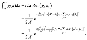
The function g(z) has only one simple pole in the complex plane, at z0 = iβγL⋆/(2A⋆). Using residue theorem in conjunction with Jordan's lemma, one has:| |  | (53) |
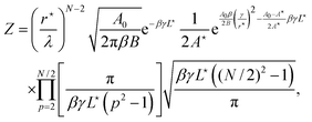
Inserting this expression into eqn (51) and integrating over the ũp≥2, one finally obtains the following expression for Z:| |  | (54) |
which is identical to the expression eqn (21).
C Jacobian
According to eqn (16), components of the Jacobian matrix ℑij associated with the change of variables ũ0,{ũp≥2} → A,{ũp≥2} are:| |  | (55) |
| |  | (56) |
Thus, ℑij is triangular with one diagonal element equal to 1/2A⋆, and the others equals to 1. Therefore, |ℑ| = 1/2A⋆.
D Modification to the update rule in the CC3D software
In the cellular Potts model, the system evolves by successive changes to the labels of the lattice sites. At each step, a random site is selected, a new target label is randomly selected amongst this site's neighboring labels, and the update is accepted or discarded following the Metropolis rule. In the standard CC3D code, the target label is chosen amongst the four first neighbors (Fig. 2) with equal weights. This criterion doesn't satisfy the detailed balance equation,14 and was thus modified according to the following procedure, which ensures proper canonical sampling.
The list of unique labels amongst the neighbors is first recorded. If multiple neighboring sites have the same label, this label only appears once in the list. The target label is then randomly selected in that list, with an even probability. This setup ends up being different than the one in the standard CC3D code, as if a label appears multiple times amongst the neighboring sites, it will not be more likely to be chosen than if it only appears once.
Acknowledgements
ANR (Agence Nationale de la Recherche) and CGI (Commissariat à l'Investissement d'Avenir) are gratefully acknowledged for their financial support of this work through Labex SEAM (Science and Engineering for Advanced Materials and devices), ANR-10-LABX-0096 and ANR-18-IDEX-0001.
References
- A. K. Doerr, M. Tolan, W. Prange, J.-P. Schlomka, T. Seydel, W. Press, D. Smilgies and B. Struth, Phys. Rev. Lett., 1999, 83, 3470–3473 CrossRef CAS.
-
J. Rowlinson and B. Widom, Molecular Theory of Capillarity, Dover Publications, 2002 Search PubMed.
- D. G. A. L. Aarts, M. Schmidt and H. N. W. Lekkerkerker, Science, 2004, 304, 847–850 CrossRef CAS.
- D. Langevin, Colloids Surf., 1990, 43, 121–131 CrossRef CAS.
- S. T. Milner and S. A. Safran, Phys. Rev. A: At., Mol., Opt. Phys., 1987, 36, 4371–4379 CrossRef CAS.
- H. Gang, A. H. Krall and D. A. Weitz, Phys. Rev. Lett., 1994, 73, 3435–3438 CrossRef CAS.
- W. Cai, Phys. Rev. E: Stat. Phys., Plasmas, Fluids, Relat. Interdiscip. Top., 1996, 54, 2780–2785 CrossRef CAS.
- E. Hannezo, J. Prost and J.-F. Joanny, Proc. Natl. Acad. Sci. U. S. A., 2014, 111, 27–32 CrossRef CAS.
- F. Graner and J. A. Glazier, Phys. Rev. Lett., 1992, 69, 2013–2016 CrossRef CAS.
- D. B. Staple, R. Farhadifar, J. C. Röper, B. Aigouy, S. Eaton and F. Jülicher, Eur. Phys. J. E: Soft Matter Biol. Phys., 2010, 33, 117–127 CrossRef CAS.
- D. Bi, J. H. Lopez, J. M. Schwarz and M. L. Manning, Nat. Phys., 2015, 11, 1074–1079 Search PubMed.
- M. Durand and J. Heu, Phys. Rev. Lett., 2019, 123, 188001 CrossRef CAS.
- S. Ljunggren and J. C. Eriksson, J. Chem. Soc., Faraday Trans. 2, 1984, 80, 489–497 RSC.
- M. Durand and E. Guesnet, Comput. Phys. Commun., 2016, 208, 54–63 CrossRef CAS.
- J. A. Glazier, M. P. Anderson and G. S. Grest, Philos. Mag. B, 1990, 62, 615–645 CAS.
- Y. Jiang, P. J. Swart, A. Saxena, M. Asipauskas and J. A. Glazier, Phys. Rev. E: Stat. Phys., Plasmas, Fluids, Relat. Interdiscip. Top., 1999, 59, 5819 CrossRef CAS.
- A. J. Kabla, J. R. Soc., Interface, 2012, 9, 3268–3278 CrossRef.
- T. Hirashima, E. G. Rens and R. M. H. Merks, Dev., Growth Differ., 2017, 59, 329–339 CrossRef.
- R. Magno, V. A. Grieneisen and A. F. Marée, BMC Biophys., 2015, 8(8) DOI:10.1186/s13628-015-0022-x.
- J. Käfer, T. Hayashi, A. F. Marée, R. W. Carthew and F. Graner, Proc. Natl. Acad. Sci. U. S. A., 2007, 104, 18549–18554 CrossRef.
- P. Marmottant, A. Mgharbel, J. Käfer, B. Audren, J.-P. Rieu, J.-C. Vial, B. Van Der Sanden, A. F. Marée, F. Graner and H. Delanoë-Ayari, Proc. Natl. Acad. Sci. U. S. A., 2009, 106, 17271–17275 CrossRef CAS.
-
M. H. Swat, G. L. Thomas, J. M. Belmonte, A. Shirinifard, D. Hmeljak and J. A. Glazier, Computational Methods in Cell Biology, Academic Press, 2012, vol. 110, pp. 325–366 Search PubMed.
- J. D. Chodera, J. Chem. Theory Comput., 2016, 12, 1799–1805 CrossRef CAS.
- O. Farago and P. Pincus, Eur. Phys. J. E: Soft Matter Biol. Phys., 2003, 11, 399–408 CrossRef CAS.
|
| This journal is © The Royal Society of Chemistry 2020 |
Click here to see how this site uses Cookies. View our privacy policy here.  Open Access Article
 *
*
![[script letter H]](https://www.rsc.org/images/entities/char_e142.gif) =
= ![[script letter H]](https://www.rsc.org/images/entities/char_e142.gif) b +
b + ![[script letter H]](https://www.rsc.org/images/entities/char_e142.gif) c.
c.![[script letter H]](https://www.rsc.org/images/entities/char_e142.gif) b = γL, where γ is the line tension (i.e. surface tension times the transverse height), and
b = γL, where γ is the line tension (i.e. surface tension times the transverse height), and  is the (fluctuating) contour length. The second contribution is the bulk compressive energy:

 . We consider here the low compressibility (ε ≪ 1) and low fluctuations (η ≪ 1) regime. In order to derive an analytical expression for the partition function, we need to expand the Hamiltonian around a reference configuration that we determine below.
![[script letter H]](https://www.rsc.org/images/entities/char_e142.gif) [rc(θ)] is a constant r⋆. Minimization of the Hamiltonian with respect to rc(θ) leads to
[rc(θ)] is a constant r⋆. Minimization of the Hamiltonian with respect to rc(θ) leads to
![[r with combining tilde]](https://www.rsc.org/images/entities/i_char_0072_0303.gif) = r⋆/r0, eqn (4) rewrites:
= r⋆/r0, eqn (4) rewrites:![[r with combining tilde]](https://www.rsc.org/images/entities/i_char_0072_0303.gif) 3 −
3 − ![[r with combining tilde]](https://www.rsc.org/images/entities/i_char_0072_0303.gif) + ε = 0.
+ ε = 0. , which then defines the stability criterion for the circular droplet: when ε > εc, the droplet collapses. When ε < εc, there are two positive roots which correspond to a maximum and a minimum of the energy, respectively. The latter corresponds to the stable configuration, and expresses as:

![[script letter H]](https://www.rsc.org/images/entities/h3_char_e142.gif)


![[scr O, script letter O]](https://www.rsc.org/images/entities/char_e52e.gif) (|ũp|4) in the Hamiltonian makes the evaluation of Z more difficult than in the incompressible case. One way to tackle this problem is by using the Hubbard–Stratonovich transformation to linearize the (A − A0)2 term in eqn (13). This method is developed in Appendix B. Here we choose another method, which consists in making the change of variables ũ0,{ũp≥2} → A,{ũp≥2} in order to express Z as Gaussian integrals. The fact that the two methods give the same expression for Z increases our confidence in the final result. We express ũ0 in terms of the new set of variables by solving the second order eqn (12). Assuming low compressibility and small fluctuations (|A − A⋆|/A⋆ ≪ 1, |ũp≥2| ≪ 1), the only physical root simplifies to:
(|ũp|4) in the Hamiltonian makes the evaluation of Z more difficult than in the incompressible case. One way to tackle this problem is by using the Hubbard–Stratonovich transformation to linearize the (A − A0)2 term in eqn (13). This method is developed in Appendix B. Here we choose another method, which consists in making the change of variables ũ0,{ũp≥2} → A,{ũp≥2} in order to express Z as Gaussian integrals. The fact that the two methods give the same expression for Z increases our confidence in the final result. We express ũ0 in terms of the new set of variables by solving the second order eqn (12). Assuming low compressibility and small fluctuations (|A − A⋆|/A⋆ ≪ 1, |ũp≥2| ≪ 1), the only physical root simplifies to:
![[scr O, script letter O]](https://www.rsc.org/images/entities/char_e52e.gif) (((A − A⋆)/A⋆)2), has a negligible contribution to the Hamiltonian in comparison with the compression term
(((A − A⋆)/A⋆)2), has a negligible contribution to the Hamiltonian in comparison with the compression term  . Inserting eqn (16) into eqn (11), we finally obtain the expression of
 ![[script letter H]](https://www.rsc.org/images/entities/char_e142.gif) in terms of the new set of variables:
in terms of the new set of variables:


 . One can then expand the range of the integral to the real axis, yielding:
![[thin space (1/6-em)]](https://www.rsc.org/images/entities/char_2009.gif) ln
ln![[thin space (1/6-em)]](https://www.rsc.org/images/entities/char_2009.gif) Z has for expression (up to additive constants):
Z has for expression (up to additive constants):


 (considering A⋆, L⋆, r⋆ as constants). It comes:


 in the space of variables Xi (1 ≤ i ≤ N − 2), with:
  ,
,  for 1 ≤ k ≤ N/2 − 1, and
  for 1 ≤ k ≤ N/2 − 2. The volume occupied by one state remains uniform through this linear change of variables. Therefore,


 , it comes:

![[scr N, script letter N]](https://www.rsc.org/images/entities/char_e52d.gif) c(k), and σk, σl are the cell IDs of site k and l, respectively. δ is the Kronecker delta symbol: δm,n = 1 if m = n, and 0 otherwise. The coupling constant J > 0 sets the amplitude of surface tension. As the range of the coupling neighborhood increases, the estimation of contact energy is smoother and gradually erases the square lattice anisotropy. However, we show below that this also generates a slight dependence of the effective surface tension with simulation temperature.
c(k), and σk, σl are the cell IDs of site k and l, respectively. δ is the Kronecker delta symbol: δm,n = 1 if m = n, and 0 otherwise. The coupling constant J > 0 sets the amplitude of surface tension. As the range of the coupling neighborhood increases, the estimation of contact energy is smoother and gradually erases the square lattice anisotropy. However, we show below that this also generates a slight dependence of the effective surface tension with simulation temperature.
 , i.e. the boundary energy measured for a unit coupling constant, divided by the boundary thickness z. Accordingly, surface tension is given by γ = zJ (in units of energy per pixel2). Roughly, z is equal to half of the number of sites in the coupling neighborhood. Actually, because of the anisotropy of the underlying lattice, z – and so γ – slightly depend on the contour shape: their values will be different for a square and a circular contour. Values of z reported in the literature range from 10.5 to 11.319–21 for 4th order coupling neighborhood, which has 20 neighboring lattice sites (see Fig. 2). Here we propose to take advantage of the thermal fluctuations of the contour and perform statistical averaging to lessen this dependency on contour shape, and determine an accurate value for z.
![[scr N, script letter N]](https://www.rsc.org/images/entities/char_e52d.gif) c for computing the boundary energy (eqn (38)).
c for computing the boundary energy (eqn (38)).![[scr N, script letter N]](https://www.rsc.org/images/entities/char_e52d.gif) c, used for calculation of the boundary energy is the order IV neighborhood, with 20 neighbors for each pixel. The target neighborhood, in which the target value is chosen from in the site updating rule of the Metropolis-like algorithm, is the order I neighborhood, with 4 neighbors per pixel (see Fig. 2).
c, used for calculation of the boundary energy is the order IV neighborhood, with 20 neighbors for each pixel. The target neighborhood, in which the target value is chosen from in the site updating rule of the Metropolis-like algorithm, is the order I neighborhood, with 4 neighbors per pixel (see Fig. 2).![[script letter H]](https://www.rsc.org/images/entities/char_e142.gif) b/J, the calibrated length being L = L′/z, and we rewrite eqn (24), (25), (27), (28), (33) and (34) in terms of the dimensionless variables ε′ = J/Br0 and η′ = kBT/Jr0, rather than ε = zε′, η = η′/z. Using expansion eqn (7) for r⋆, we obtain:
b/J, the calibrated length being L = L′/z, and we rewrite eqn (24), (25), (27), (28), (33) and (34) in terms of the dimensionless variables ε′ = J/Br0 and η′ = kBT/Jr0, rather than ε = zε′, η = η′/z. Using expansion eqn (7) for r⋆, we obtain:


 . It can be noticed that the distribution of area, perimeter and energy are all affected by the finite compressibility of the droplet.


 , and then evaluate ũp from eqn (10). Fig. 8 shows the variation of 〈|ũp2|〉 with p. Again, data are well predicted by the theoretical expression eqn (35), and yields for the unique fit parameter z = 10.88, consistent with values obtained from other expressions (see Fig. 4). We also reported on the graph −4〈ũ0〉/9 calculated with this value of z. In agreement with eqn (37), its value is very close to 〈|ũ2|〉2.
![[scr O, script letter O]](https://www.rsc.org/images/entities/char_e52e.gif) (ε,η). Values of z and a excerpt from the different fits are consistent with each other. However, we noticed a small decay of z – and hence the CPM surface tension – with the amplitude of thermal fluctuations. We suspect that this thermal softening of surface tension is caused by the short wavelength fluctuating modes: for modes whose wavelength is shorter than the range of interactions between lattice sites (set by the size of coupling neighborhood), the number of unlike lattice sites in the coupling neighborhood of a given site at the boundary is smaller than the one expected for a flat interface. To test this hypothesis, we calculated z explicitly for static configurations of a droplet with modulated radius rc(θ) = r⋆(1 + 0.025
(ε,η). Values of z and a excerpt from the different fits are consistent with each other. However, we noticed a small decay of z – and hence the CPM surface tension – with the amplitude of thermal fluctuations. We suspect that this thermal softening of surface tension is caused by the short wavelength fluctuating modes: for modes whose wavelength is shorter than the range of interactions between lattice sites (set by the size of coupling neighborhood), the number of unlike lattice sites in the coupling neighborhood of a given site at the boundary is smaller than the one expected for a flat interface. To test this hypothesis, we calculated z explicitly for static configurations of a droplet with modulated radius rc(θ) = r⋆(1 + 0.025![[thin space (1/6-em)]](https://www.rsc.org/images/entities/char_2009.gif) cos(2πr⋆θ/λ)) and discretized on a square lattice, with r⋆ = 30 pixels, for varying wavelength λ. Results are shown in Fig. 9: for modes with λ ≳ 10 pixels, z does not really depart from a constant value ≃11.3. For modes with shorter wavelengths, z decreases monotonically down to 10.5. It can be noticed that this range of z values coincides with the range of values reported in literature. This thermal softening effect could then rationalize the scattered values of z found in literature. Moreover, as the thermal softening of the CPM surface tension is caused by the fluctuating modes with wavelength comparable or shorter than the range of lattice site interactions, we expect this effect to be more pronounced when the coupling neighborhood is increased. Hence, the choice for its size should be the result of a trade-off between reducing anisotropy and limiting this unexpected temperature dependence. Presumably this dependence is enhanced in our version of the algorithm that satisfies detailed balance (see Appendix D): consider a rugosity of one single site, on an otherwise flat interface. This site is surrounded by three sites in its target neighborhood having dissimilar labels, and a single one that shares the same label. In the original algorithm, the unlike label is three times more likely to be chosen as the target label than the similar one, whereas they have equal probabilities in the modified version. The rugosity is therefore more likely to be smoothed out in the unmodified version. As rugosities with short wavelengths are the leading cause of thermal softening, this effect is less pronounced when interfaces are flattened.
cos(2πr⋆θ/λ)) and discretized on a square lattice, with r⋆ = 30 pixels, for varying wavelength λ. Results are shown in Fig. 9: for modes with λ ≳ 10 pixels, z does not really depart from a constant value ≃11.3. For modes with shorter wavelengths, z decreases monotonically down to 10.5. It can be noticed that this range of z values coincides with the range of values reported in literature. This thermal softening effect could then rationalize the scattered values of z found in literature. Moreover, as the thermal softening of the CPM surface tension is caused by the fluctuating modes with wavelength comparable or shorter than the range of lattice site interactions, we expect this effect to be more pronounced when the coupling neighborhood is increased. Hence, the choice for its size should be the result of a trade-off between reducing anisotropy and limiting this unexpected temperature dependence. Presumably this dependence is enhanced in our version of the algorithm that satisfies detailed balance (see Appendix D): consider a rugosity of one single site, on an otherwise flat interface. This site is surrounded by three sites in its target neighborhood having dissimilar labels, and a single one that shares the same label. In the original algorithm, the unlike label is three times more likely to be chosen as the target label than the similar one, whereas they have equal probabilities in the modified version. The rugosity is therefore more likely to be smoothed out in the unmodified version. As rugosities with short wavelengths are the leading cause of thermal softening, this effect is less pronounced when interfaces are flattened.

![[thin space (1/6-em)]](https://www.rsc.org/images/entities/char_2009.gif) cos(2πr⋆θ/λ)) as a function of wavelength λ.
cos(2πr⋆θ/λ)) as a function of wavelength λ.![[script letter H]](https://www.rsc.org/images/entities/h3_char_e142.gif)
![[script letter H]](https://www.rsc.org/images/entities/char_e142.gif) [rc(θ)] is defined by gathering all configurations corresponding to a given shape of the droplet, specified by its contour rc(θ):
[rc(θ)] is defined by gathering all configurations corresponding to a given shape of the droplet, specified by its contour rc(θ):
![[script letter H]](https://www.rsc.org/images/entities/char_e142.gif) c, and a boundary contribution
c, and a boundary contribution ![[script letter H]](https://www.rsc.org/images/entities/char_e142.gif) b. When the thermalization of the inner fluid is much faster than the typical boundary displacements, we can identify
b. When the thermalization of the inner fluid is much faster than the typical boundary displacements, we can identify ![[script letter H]](https://www.rsc.org/images/entities/char_e142.gif) c with the Gibbs free energy of the compressible fluid.
c with the Gibbs free energy of the compressible fluid. ![[script letter H]](https://www.rsc.org/images/entities/char_e142.gif) c then does not depend on the specific shape of the droplet, but on its area A only. The pressure difference between the inner and outer fluids is given by P − P0 = −
c then does not depend on the specific shape of the droplet, but on its area A only. The pressure difference between the inner and outer fluids is given by P − P0 = −![[script letter H]](https://www.rsc.org/images/entities/char_e142.gif) ′c(A)/h, where h is the transverse height of the droplet. Expanding
′c(A)/h, where h is the transverse height of the droplet. Expanding ![[script letter H]](https://www.rsc.org/images/entities/char_e142.gif) c(A) around the nominal value A0, which corresponds to the area value for which P = P0, we get:
c(A) around the nominal value A0, which corresponds to the area value for which P = P0, we get:
![[script letter H]](https://www.rsc.org/images/entities/char_e142.gif) ′′c(A0) is the 2D bulk modulus of the inner fluid measured at pressure equal to the surrounding pressure (P = P0). Note that the compressive energy is minimal when the inner pressure and area match their outer counterparts. The additive constant
′′c(A0) is the 2D bulk modulus of the inner fluid measured at pressure equal to the surrounding pressure (P = P0). Note that the compressive energy is minimal when the inner pressure and area match their outer counterparts. The additive constant ![[script letter H]](https://www.rsc.org/images/entities/char_e142.gif) c(A0) has been dropped in eqn (2).
c(A0) has been dropped in eqn (2).
![[script letter H]](https://www.rsc.org/images/entities/char_e142.gif) b = γ
b = γ![[script L]](https://www.rsc.org/images/entities/char_e144.gif) ;
; ![[script letter H]](https://www.rsc.org/images/entities/char_e142.gif) b does not depend on the specific shape of the droplet either, but only on its perimeter
b does not depend on the specific shape of the droplet either, but only on its perimeter ![[script L]](https://www.rsc.org/images/entities/char_e144.gif) . Note that this expression implies that surface tension γ is uniform; if the droplet boundary contains surfactant molecules, it is then assumed that fluctuations of their surface concentration can be neglected.
. Note that this expression implies that surface tension γ is uniform; if the droplet boundary contains surfactant molecules, it is then assumed that fluctuations of their surface concentration can be neglected.


 , it cannot be switched with the integral over ũ0. This peculiarity is specific to the case studied here: it does not arise when adding bending term in the energy,24 or for an initially flat geometry, or even when using fixed boundary conditions rather than periodic ones. To compute Z, we first calculate Z(
![[small script l]](https://www.rsc.org/images/entities/char_e146.gif) ), which is defined identically to Z, except for the integration over ũ0 which is restricted to the domain [−
), which is defined identically to Z, except for the integration over ũ0 which is restricted to the domain [−![[small script l]](https://www.rsc.org/images/entities/char_e146.gif) ,+∞]. Z will then be deduced from Z(
,+∞]. Z will then be deduced from Z(![[small script l]](https://www.rsc.org/images/entities/char_e146.gif) ) using
) using  . Integrals over k and ũ0 can then be switched, and integration over the latter yields:

