Self-assembly of charged colloidal cubes

Abstract

In this work, we show how and why the interactions between charged cubic colloids range from radially isotropic to strongly directionally anisotropic, depending on tuneable factors. Using molecular dynamics simulations, we illustrate the effects of typical solvents to complement experimental investigations of cube assembly. We find that in low-salinity water solutions, where cube self-assembly is observed, the colloidal shape anisotropy leads to the strongest attraction along the corner-to-corner line, followed by edge-to-edge, with a face-to-face configuration of the cubes only becoming energetically favorable after the colloids have collapsed into the van der Waals attraction minimum. Analysing the potential of mean force between colloids with varied cubicity, we identify the origin of the asymmetric microstructures seen in experiment.

---

1 Introduction

For over 70 years, the classical works of Derjagin, Landau,¹ Vervey and Overbeek² have formed the paradigm that is used to understand the interparticle interactions when investigating the behaviour of colloidal systems dominated by electrostatic and van der Waals interactions.^3–6 Commonly referred to as Derjaguin–Landau–Verwey–Overbeek theory, their model predicts a strong qualitative dependence of colloidal interactions on the surface charge density. At small distances, the van der Waals attraction between two particles exceeds the double layer repulsion, resulting in assembly. Yet to reach such distances, the two surfaces must first overcome an energy barrier that may be prohibitively high. The key to the stability of these systems therefore lies in the existence and height of the barrier. In systems with comparable double layer overlap forces and van der Waals attraction, this potential may also possess a secondary minimum. Aside from the clear dependency on the surface charge, the existence and extent of these features are again affected by the choice of electrolyte, which influences the screening of the double layer overlap forces^7,8 and the strength of the van der Waals attraction.⁹

Despite the ubiquity of DLVO theory, it is not sufficient to predict colloidal self-assembly even in systems of spherical colloids. It has been shown that even in the framework of DLVO theory, various phase transitions^10–12 or even hard-sphere behaviour⁶ can be found in such systems. Furthermore, direct measurements of the interactions between three charged colloids revealed that the forces already begin to deviate from a standard mean-field approach for relatively small intercolloidal distances, even in systems with only monovalent ions.¹³

If one investigates systems of multivalent ions, the phase behaviour of charged spherical colloids changes dramatically. One can observe the appearance of like-charge colloidal attraction with further phase separation or crystallisation.^14–20 The necessity to consider counterions explicitly fueled the development of new theoretical approaches²¹ and extensive use of computer simulations.^22,23 The distribution of counterions affects the diffusive and electrophoretic mobility of charged colloids.^24,25 Such concentration effects were thoroughly studied in ref. 26, which also reported the re-entrant freezing–melting behaviour caused by changes in the charge.

Apart from systems of like-charged spherical colloids, thorough investigations of systems of oppositely charged colloids have also been made. The focus in such studies is typically on the crystallisation process and the resulting crystalline structures.^27–29 Another type of binary mixture was investigated in ref. 30, where the colloids of like-charge but different sizes were studied. It was found that the size-ratio has a significant impact on the phase behaviour.

In addition to the effects of the charge and size of the colloids, and the valency of the counterions, the shape of the charged colloids can also play a crucial part in their phase behaviour.³¹ Systems of asymmetric colloids, such as rods, spheroids or cylinders, show anisotropy in their intercolloidal forces.^32–34 These effects can be compounded by considering flexible polyelectrolytes instead of rigid colloids.³⁵ The case of planar surfaces, whose attraction in the presence of multivalent counterions is responsible for the restricted swelling of clay and reduction in the water uptake of lamellar membranes, was thoroughly investigated in ref. 36. Another area of keen scientific interest was the phase diagram of charged platelets of the model of LAPONITE®, which has been addressed by many authors.^37–40

In recent years, colloids of different shapes including peanuts, polyhedra and superballs have become available.^41–47 When only excluded volume interactions are present in the studied systems, the shape of colloids is able to alter the mechanism and outcomes of the assembly processes.^48–53 Additional electrostatic or hydrodynamic interactions as well as confinement at the interfaces bring new flavours to the phase behaviour.^54–57

By analyzing the influence of colloidal shape on the self-assembly, we can ask how strong the deviation from a spherical shape must be to have a notable impact on the macroscopic properties. This question is especially relevant for developing new materials based on controlled self-assembly.^58,59 To this extent, cubic particles become very useful, as they represent a limiting case of superballs,^60–62 whose shape can be described as

As the shape parameter q goes to infinity, a perfect cube with sharp edges is obtained. If q = 1, eqn (1) describes a sphere with radius r centered at the origin.

For perfect or truncated cubes, the phase behaviour was shown to be qualitatively different from that of spheres.^63–66 The evolution from a sphere to a cube was investigated thoroughly for the case of magnetic dipolar cubes.^67–69 It was shown that even for small values of q, such as q ∼ 1.3, the self-assembly scenario changes from ring formation for perfect spheres to chain formation for superballs. The computational approach developed for magnetic superballs was employed to describe the self-assembly of hematite cubes covered with a silica shell⁷⁰ with q ∼ 1.5. Should the hematite core be dissolved, the aforementioned shell represents a hollow silica superball, as first obtained in ref. 43.

The crystallization of hollow silica superballs can be induced by use of depletant polymers.^71,72 Depending on the solvent and salinity of the solution, hollow silica superballs can exhibit self-assembly even without additives due to the competition between electrostatic and van der Waals forces. This dovetails with the classical DLVO case mentioned above. As has been shown for systems of colloidal platelets,⁴⁰ the competition between two interactions can result in an intricate variety of colloidal behaviour. Due to the high complexity of these systems, rigorous investigations of suspensions with anisometric colloids, and superballs in particular, remain in their infancy.

Our work goes beyond such boundaries by obtaining a pair potential that can describe anisotropic interactions of charged colloidal superballs. As an analytical solution would – among other challenges – imply solving the many-body problem, we used molecular dynamics simulations based on experimental observations and parameters to recreate the system presented in Fig. 1in silico. Furthermore, we will explore possibilities to reconfigure the system by tuning properties such as solvent and salinity. By clarifying the attachment mechanism and pair potential of these cubes, we lay the foundation for further study of the resulting structures.

Fig. 1 Left: SEM micrographs of hollow silica nanocube monolayers obtained from Langmuir–Blodgett deposition. On the right, a close-up micrograph of the monolayer depicted on the left.

The manuscript is structured as follows. We first describe the experimental and simulation methods (Section 2). The following section, “Results and discussion”, begins by characterizing the electrostatics of a single superball with a shape parameter of q = 1.7 by computing the counterion distribution and field intensity around it. In the subsequent Section 3.2, we move to investigating the assembly process of pairs of colloids. We calculate the interaction potential along those symmetry axes and analyse how the balance between van der Waals attraction and electrostatics affects it. Comparing simulation results to experimental observations, we explain the preferred corner-to-corner contact observed for hollow silica superballs. We generalise our study for different salinities of solutions and cubicity of colloids in them in Section 3.3. We summarise our findings in Section 4.

2 Model and methods

2.1 Experimental methods

2.1.1 Preparation of hollow silica nanocubes. Hollow silica nanocubes were obtained as discussed by Dekker et al.⁴⁷ Here, we provide a brief summary. Cuprous oxide nanocubes⁷³ were obtained by a water-assisted Polyol method resulting in a Cu₂O nanocube with an edge-length of 103 ± 10 nm. The obtained nanocubes were subsequently coated with a 13 nm thick silica shell using the PVP-assisted Stöber method.^74,75 In the final step, the cuprous oxide core was removed by dissolving the core in HNO₃/HCl, obtaining hollow SiO₂ nanocubes with an edge length of 128 ± 11 nm and a q value of ∼1.7–1.8. The particles are depicted in Fig. 2. As described in ref. 76–78, cubes with other values of q were also synthesized, but were not studied that extensively. The results provided below profit from the complimentary simulations.

Fig. 2 (left) Cu₂O nanocubes with an edge length of 103 ± 10 nm. (middle) Cu₂O particles coated with a 13 nm SiO₂ shell. (right) Hollow SiO₂ particles with an edge length of 128 ± 10 nm and the value of q ∼ 1.7–1.8 obtained from the particles in the middle.

2.1.2 Monolayer preparation. Monolayers of hollow silica nanocubes were obtained using a KSV-Nima Langmuir Trough equipped with a dip-coater. In short, particles in a 2 : 1 (weight : weight) mixture of cyclohexane:ethanol were spread on an aqueous 1 mM KCl solution. After 10 minutes of equilibrating, the monolayer was compressed with a speed of 10 cm min⁻¹. The formed monolayers were transferred to a hydrophilized glass slide by dip-coating. The monolayer was inspected using an Xl30feg scanning electron microscope. Monolayers are important for visualisation, however a vast part of the cube's characterisation using Small Angle Neutron Scattering was performed on the bulk.^76–78

2.2 Simulation model

2.2.1 Generic simulation details. Simulations were performed in the NVT ensemble, using the Molecular Dynamics software package ESPResSo-3.3.1.⁷⁹ Among other features, it provides an implementation of the Lennard-Jones and Debye–Hueckel pair potentials used and the Langevin thermostat with which the temperature was regulated. In order to facilitate comparison with experimental results, the simulation temperature k_BT was scaled such that k_BT = 1 corresponded to 1 zJ. All simulations were run at k_BT = 4. As mentioned above, we are interested in the fundamental understanding of the shape-impact on the self-assembly scenario of the charged cubes, thus we focus here on bulk systems. This helps us to avoid additional effects caused by the presence of an interface.^80,81 The choice of parameters presented below is in agreement with our earlier investigations⁸² and known experimental data.⁸³

To model the van der Waals attraction between colloids, the Lennard-Jones potential is used. In the cases of interacting particles without any attraction (ions, surface charges), the Weeks–Chandler–Anderson⁸⁴ potential provided the required steric repulsion. Here, σ is the diameter and ε is the energy scale parameter, which corresponds to the well depth. For particles with different diameters, σ was calculated by using the Lorentz(–Berthelot) rules.

This work used explicit surface charges and an equal number of counterions to ensure overall charge neutrality. However, since the solvent was not modeled explicitly, the Debye–Hueckel potential was used in place of the pure Coloumb interaction. This allows us to tune the Bjerrum length l_B to mimic the varying dielectric of different solvents, as well as the Debye length κ⁻¹, which mimics the screening of charges at distance r in a solvent due to salt ions.

In this work, l_B was set to 0.71 for simulations of water and 2.28 for ethanol. For the Debye length in dependence of the ionic strength, we used κ⁻¹(10⁻³) = 9.63 and κ⁻¹(10⁻⁴) = 30.44. Both of these values were obtained by computing l_B and κ⁻¹ from their definitions (see ref. 8), then rescaling into simulation units. As all ions are presumed to be monovalent, all surface charges were set to q_S = −1 and, for counterions, q_CI = 1.

2.2.2 Modelling of a single cube. The cubes were represented using the superball model developed by Donaldson et al., see ref. 68. To model the charged surface, we added explicit point charges placed on the analytical surface of the superball. In order to conserve the symmetry found in experiment, the charges were placed by wrapping a 2D grid onto the surface of each superball face. Given the experimentally known surface charge of S = 5–10 × 10³ charges per nm², we obtain roughly 81 charges per face. Once this was corrected to consider that each face's grid would assign a charge to each bordering corner, leading to three charges per corner, the total number of charges became 470 per superball. The result is shown in Fig. 3(a). Placing the charges on the analytical surface also leads to their centers protruding slightly above the cube-composing spheres in many areas. This is intentional, to allow counterions to settle on the surface without being pushed away during assembly. The slight offset of the grid and the choice to compose the surface of several different spheres with different extensions mimic the reality that such silica cubes are bumpy and porous.

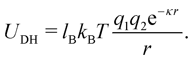
Fig. 3 (a) A single simulation superball, with the central sphere in light blue, the edge-composing spheres in white and the corner spheres in light green. On the right half of the cube, we see the added point charges in turquoise. The grid between the charges is shown for illustrative purposes only. (b) The three main types of symmetry axes of a cube, along which the cubes are aligned during the assembly routine. Blue indicates the symmetry axis through the centers of two opposite cube faces, purple indicates that through the centers of two opposite cube edges and green indicates the axis through two opposite cube corners.

The diameter σ of the central sphere was set to 90 simulation length units, with the edge and corner spheres scaled in accordance with ref. 68. This means that the “height” of a simulation cube is 90. The surface charges and corresponding explicit counterions were given the diameter σ_c = 1 to correspond to their hydrodynamic radius. To accommodate both of these very particle length scales on the same timescale, cubes were given a simulation mass and inertia. The simulation mass of the cubes was chosen to be m = 50 based on tuning, with the corresponding moments of rotational intertia for a hollow cube computed to be I = 675 000 along each axis.

The spheres simulated for comparison had a diameter of 90, with an amount of charge calculated to match the surface charge density of the spheres (254) distributed using a 3D Fibonacci spiral pattern. The number of counterions was also adjusted to match. Since these spheres were only used in the fixed simulations, they did not require masses or inertia.

For the alternative shapes q = 1.3, q = 2.0 and q = 3.0 shown later in the work, we kept the total charge, mass, inertia and all other parameters identical to the q = 1.7 case, with two technical exceptions. First, the grid had to be modified slightly for the greater surface area for q = 3.0 and the lesser surface area for q = 1.3. To ensure comparability to the q = 2.0 case, we rescaled the surface charges and counterion charges. Secondly, we had to include two additional spheres per edge in the edges for the q = 3.0 case to mimic the higher curvature.

2.2.3 Single cube systems. For the density profiles and field measurements, a single cube was fixed in the center of a simulation box of size 270. A number of counterions equal to the number of surface charges (470) were randomly placed inside the box. To determine the amount of integrations to equilibrate, the system was set to t = 20 000Δt, where Δt = 0.01, based on several test runs. From that point on, the system was sampled at intervals of 100 000 integrations to ensure statistical independence. We also varied the overall charge density by increasing the box size to 360, 450 and 540. This quantitatively decreased the layer height, but did not qualitatively change the results. We also chose not to pursue the variation of charge densities, as the qualitative anisometry effects were shown to hold regardless of the concentration of counterions near the cube.
Density profiles. The density profiles, presented below, are computed by counting the number of counterions in a given area (bin) at a given distance away from the feature, then normalized by the volume of the bin (for comparison across distances), and the total number of counterions (for comparison across shapes). The shape of these bins was adapted to the shape of the feature: for spheres, it is trivial to see that the bins are spherical shells. Likewise, the bins corresponding to faces were chosen as a series of rectangles parallel to the surface. For corners, the situation resembles that of sphere – we are essentially computing the radial distance to a specific point. However, due to the proximity of edges in corners, not all counterions should be considered. To distinguish between the effects caused by different features, we only select the counterions above a plane through the center of the corner sphere, orthogonal to the cube's symmetry axis. This reduces our spherical bins to hemispheres. This leaves the distribution around edges. To measure the distance to edges, we chose the in-plane distance between the counterion and the point of the edge at the same height. Combined with the necessity for averaging over the different heights, this gives us concentric cylindrical bins. To exclude the counterions attached to the cube faces, we reuse the plane approach. In this case, the plane passes through the edge and is chosen orthogonal to the symmetry axis through the center of the cube edge. This reduces the bins to half-cylinders. The results for each direction were averaged over 79 checkpoints, taken at intervals of 100 000Δt.
Fields. To measure the electric field strength at any specific point in the system, we implemented a computational version of the test charge definition of the field. A single positive unit charge is placed at the point of interest, and, after a brief check for steric overlap, the forces on this charge are evaluated. Due to the computational cost of this routine, only ten checkpoints were used.

2.2.4 Two cube systems. Two different kinds of simulations were run to obtain the results shown in the last part of the Results and discussion section. The first variant consisted of placing two cubes with their surrounding counterion clouds into a simulation box at a center to center distance less than two cube lengths, then equilibrating the system. This resulted in the self-assembling of cubes, the mechanism of which could be observed in the trajectory files.

For the potential measurements, a pair of cubes was aligned along one of the three axes shown in Fig. 3(b) and fixed at a center to center distance r. Then, the counterions were allowed to equilibrate for 2 000 000Δt, where Δt = 0.001. From this point on, measurements of the projection of the force along the axis along which the cubes were aligned were taken every 100 000Δt. The result was averaged over 100 measurements, then integrated numerically by taking the mean value of the upper and lower Darboux sums.

3 Results and discussions

3.1 Single superball

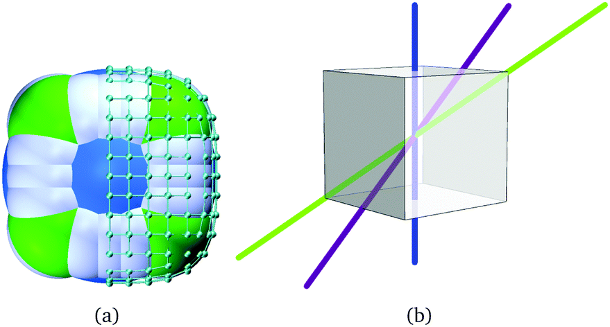
We first examine a system containing a single colloid surrounded by counterions in an implicit solvent with a dielectric constant corresponding to that of water. To analyse the effect of the colloidal anisotropy, we compute the distribution of counterions, φ, near the faces, edges and corners of the superball as well as surrounding a reference sphere. Based on the varying ionic concentrations used in experiment, we altered the screening length to mimic the effects of a monovalent salt. The results for high, low and intermediate values of salinity are summarized in Fig. 4(a)–(c). In Fig. 4(d), the counterion distribution for a cube in ethanol is presented.

Fig. 4 Density profiles of counterions (top row) and field intensity colour maps (bottom row) in (a and e) water with no salt or monovalent salt with an ionic concentration of 10⁻⁷ molar, (b and f) water with a monovalent salt concentration of 10⁻⁴ molar, (c and g) water with a monovalent salt concentration of 10⁻³ molar (highest concentration used experimentally) and (d and h) ethanol. Density profiles are calculated from cube faces (blue), corners (green) and edges (purple), as shown in Fig. 6(b). The corresponding counterion distributions for a spherical colloid are in gray. In the top row of plots, (a–d), r_s refers to the distance between the counterion center and the surface of the colloid. The field intensity plots each depict the magnitude of the vector valued electric field in simulation units at the points shown, where the unit charge is set to e₀ = 1. The left half of each image depicts the field around a spherical colloid centered at (0,0), while the right half contrasts this with a cubic colloid centered at (0,0). The labels on the x and y axis refer to distances in nm.

For low salinity, as presented in Fig. 4(a), we see the formation of an electric double layer surrounding the colloid. For each type of cube feature, we see clear differences with respect to the reference sphere. The layer appears much more pronounced in the profiles of cube faces than edges or corners. This shape also varies for different geometric features of the cube in question, showing that the anisometry of the underlying particle gives rise to an asymmetric counterion distribution around it. At a scaling that allows us to view the profiles of all features together, those of the edges and corners appear barely distinguishable. Closer examination reveals the distribution near the edges to have a slightly higher peak (more face-like shape) than that of the spheres. Additionally, with gray symbols, we show the density profile around a spherical colloid with the same surface charge. For all geometries, examination of larger systems showed that the profile collapses into approximate equidistribution (allowing for thermal fluctuations) from roughly 100 nm past the surface on, which is why only that region is depicted.

Moving to higher salinities, as shown in Fig. 4(b) and (c), the screening practically nullifies the field near the cube. For the highest salt concentration (Fig. 4(c)), the density profile from the cube face coincides with that of a spherical colloid.

Moving to ethanol as the solvent, as depicted in Fig. 4(d), we obtain a layer consisting of far more counterions very close to the cubes. Noticeably, the peaks for each of the density profiles are more localized and the curves are smoother even across comparable length scales. This may be caused by the stronger double layer overlap forces dampening the effects of the Brownian motion of the particles. While the profiles near different features (exempting edges and corners) still differ quantitatively, the shapes resemble each-other to the extent that they could be considered identical.

We also measured the electric field strength near the colloid with a test charge method. In order to underline the influence of anisometry on the electrostatics of a single colloid, we present colour maps of the electric field intensity in the bottom row of Fig. 4. The left sides of these maps, provided in Fig. 4(e)–(h), show the intensity calculated around a spherical colloid, whereas the right side corresponds to a superball. Here, similar to the top row, the salinity grows from Fig. 4(e)–(g). In plots of the field in ethanol, we see that the drop in the field is much more pronounced than that in water. We also see that the anisotropy appears to be conserved for slightly longer. This appears to be a result of the longer Bjerrum length allowing the effects of the surface charge to be felt farther away from the colloid. We limited the range of these evaluations to 50 nm from the surface of the colloid based on the density profiles, which show that the counterion profile reduces to spatial equidistribution past that distance. Here (bottom row, Fig. 4), we see even more clearly that the shape effects of the superball are fairly short-ranged: the inner regions of charges depicted in Fig. 4 still appear to have elongated faces that flatten into an approximately spherical region farther outwards than 30 nm.

Concluding this section, one can say that colloidal anisometry clearly manifests itself in the electrostatic properties of isolated particles. The fact that the differences in counterion density appear so pronounced between the faces and edges or corners must affect the intercolloidal interactions. This is discussed in the next section.

3.2 Pairwise interactions

The preference of nanocubes to approach each-other corner to corner is also visible in preliminary Langmuir–Blodgett experiments on hollow silica nanocubes. A monolayer of silica nanocubes, depicted in Fig. 1, was transferred from the liquid–air surface to a glass slide using the Langmuir–Blodgett technique.^76–78 In Fig. 1, the combination of side–side, corner–side and corner–corner oriented cubes is visible. Additionally, it is visible in Fig. 1 that the monolayer does not exhibit long-range order. The morphology observed in Fig. 1 clearly differs from the simple cubic, Λ₀, and Λ₁ morphologies earlier observed for cubic particles.^71,72 We surmise that upon compression, the nanocubes have a preference to approach corner–corner or corner–side, preventing the particles from forming a densely packed ordered monolayer. The observed silica nanocube monolayers obtained by the Langmuir–Blodgett method are clearly different compared to the monolayers of micron-sized silica cubes obtained from convective assembly (CA).⁷² With convective assembly, mostly close packed monolayers with long range order are obtained. During CA, particle assembly is dominated by capillary forces and solvent flow, which dominate over the subtle differences in pair-potential between corner to corner, face to face, and edge to edge approach presented in Fig. 6.

As the first effects of the anisometry on the electrostatics have been established, we move to explain the assembly mechanism seen in experiment. This begins with a computer experiment to observe the self-assembly, followed by a series of simulations to measure the forces involved and compute the pair potentials at different orientations. By generalizing these results to different solvents and salinities, we see that we can move beyond merely understanding the assembly process to controlling it by tuning the underlying electrostatic properties of the system.

Simulations of cube pairs suspended in water showed a specific, persistent pattern in the way cubes approached each-other and assembled. The three main stages of the process are illustrated in Fig. 5.

Fig. 5 Snapshots of two cubes (turquoise) surrounded by the counterions (gray) self-assembling in a specific sequence of mutual orientations. The cubes initially orient in a corner-to-corner configuration (top), then rearrange into an edge-to-edge orientation (middle) and lastly come to remain in a face-to-face configuration (bottom). A video rendering of this process is included in the ESI.†

At the beginning of the assembly process (top), cubes prefer to orient themselves corner to corner. Once the colloids are close, they rearrange into an edge to edge configuration (middle). Finally, at equilibrium, they assume the orientation that maximizes the surface area in contact, which is a slightly off-center version of face to face (bottom). This final configuration is maintained at equilibrium. This assembly mechanism ties into experimental observations that cubes show a preference for corner to corner or edge to edge configurations during assembly, although only 2D images of the process exist, which make those two kinds of orientation hard to distinguish. In our investigation of the electric double layer, we saw that the screening of the face charges strongly differs from that near cube corners or edges. It is worth mentioning that hydrodynamics is not present in our simulation scheme, whereas it is inevitable in experiment. However, we expect that the presence of solvent will make the corner-to-corner approach even more preferable. Thus, below, we focus on the impact of electrostatic and steric forces only.

To explain the dominance of the corner-to-corner approach more systematically, we measured the interparticle forces between two cubes in three different configurations: cubes approaching each other face-to-face, edge-to-edge or corner-to-corner. By integrating these forces along corresponding directions, we obtained the corresponding potential of mean force, U, measured in units of k_BT. The results are plotted in Fig. 6 for two salt concentrations and three different values of Hamaker constant as explained in the legend in the center of Fig. 6(b). First, we see that despite the faces having quantitatively the highest counterion layer, their configuration is not favorable at larger separation distances. This orientation is only adopted when the cubes are so close that other orientations begin to encounter steric repulsion, unless the Hamaker constant is so low that the directional dependence disappears. The fact that the attraction between two cubes is initially maximised in the corner to corner configuration stems from the fact that the faces have a far greater surface area (and so more charges) at closer proximity. Considering this difference, it is almost surprising that the gap between the amount of counterions near surfaces as opposed to corners and edges is not more pronounced. Indeed, this configuration only occurs when the van der Waals attraction is close to its maximum. The slight angle between assembled cube pairs has also been seen in experiment, most notably in lattices formed by such cubes.⁸⁵

Fig. 6 Potential of mean force of pairs of cubes in three key orientations in water (a), with varying strengths of the Lennard-Jones parameter (see, (b)). The parameter r refers to the center-to-center distance between approaching cubes. The legend is provided in the middle (b). Insets in (a) show close-ups of the potentials with simulation error-bars. The potentials are truncated at the distance after which the Lennard-Jones potential would create an artificial steric repulsion, roughly 5 nm before the contact distance in each configuration. (c) Experimental SEM micrograph of hollow silica nanocubes where the different configurations are highlighted. The corners are highlighted in green while the edges are highlighted in purple.

In contrast, the edge to edge configuration only appears to be favorable within a short (around 15 nm) range of distances (inset of Fig. 6(a)), although it is only slightly less attractive than the corner to corner configuration at greater distances. This could be explained by the strong distance dependence of the van der Waals attraction. Since the difference in screening between corners and edges is not as pronounced, cubes initially prefer the configuration with the lowest double layer overlap forces. Once they draw closer, the van der Waals attraction grows and can overcome the double layer overlap forces of the edges, despite their charges being less well screened than the corners.

Although the corner to corner configuration does not appear to be significantly more favorable than that of edge to edge in the potential measurement simulations, this is consistently seen in two-cube assemblies. This may be due to a modeling simplification in the measurement procedure: the fixed cubes are aligned with the corner charges approaching each-other, whereas in the trajectories, it is possible to see that the corners are not precisely in line. In Fig. 5, for instance, the cube on the left is tilted slightly towards the reader and down, while the cube on the right is tilted up. In that vein, one should also note that while the overall charge density matched that of experiment, the charges in the corners are slightly closer to each other due to the curvature of the superball.

We now have specific values for the potential to compare with the experimental and/or analytical results for similar systems. As the distance between the cubes decreases, the potential decreases to well below 100 k_BT, which makes the cube clusters very stable at room temperature. In the limits of larger separations, we see that the interaction potential goes to zero. Upon comparing to the standard DLVO-curves⁸ for spherical colloids, we find close resemblance with our face-to-face curves.

3.3 Influence of salt and colloidal shape on the pairwise interactions

As shown in Fig. 4, the effects of shape vanish with screening induced by the presence of salt. By analyzing the differences between the potentials calculated in the salt-free case (Fig. 6(a)) and their counterparts obtained in 10⁻³ molar salt solution (Fig. 4), we see that the shape effects are much weaker. Once the salinity is high enough for the electric double layer not to form, the potential becomes slightly less attractive at close ranges and the anisometry effects begin to disappear, as seen in the inset of Fig. 7. The former can be explained by the fact that at close distances, the screening due to the increased salt content is not as strong as the screening provided by the electric double layer in other systems. When examining the differences in the double layer contingent on the geometric feature of the colloid directly beneath it, we saw that the differences in double layer near edges and corners were minimal, despite edges having comparatively more charges at a lesser distance from the edge.

Fig. 7 Potential of mean force, U, of pairs of cubes in three key orientations with varying strengths of the Lennard-Jones parameter in a monovalent salt solution with an ionic concentration of I = 10⁻³ molar. The parameter r refers to the center-to-center distance; the insets again show a close-up of the potentials with error-bars and the legend is identical to that in Fig. 6(b).

This may suggest that the corner to corner approach was energetically favorable because their repulsion was more strongly screened. Without an electric double layer, the screening is independent of the colloid's shape. This would explain why the corner to corner and edge to edge configurations no longer differ energetically, although the face to face configuration is still more repulsive. This suggests that although the anisometry effect on the distribution of ions can be tuned by changing the salinity, there is no experimentally attainable salt concentration at which the pair potential becomes independent of cube orientation. These potentials show a pronounced gap between different salinities, which slowly decreases as the potential goes to zero. Overall, differences in the ionic concentration of salt in the solvent do not show a strong affect on the interaction potential of cubes, except in the (experimental) limit cases. The scale of the attraction is still determined by the value of ε and is comparable to that in Fig. 6.

Our previous findings suggest that inhomogenity of the electric field close to the cube surface causes anisotropy of counterion density profiles to be specifically pronounced for low-salinity solutions, leading to the existence of a preferred orientation for two cubes to approach each other, namely corner-to-corner. In order to consolidate this conclusion, we performed simulations for superballs with q = 1.3, 2.0 and 3.0 and a fixed total charge, equal to that studied above for q = 1.7. All these values of q are accessible in experiment,^76–78 albeit they have not been investigated in detail yet.

First, as in the case of the readily experimentally available system analysed above, in Fig. 8, we depict density profiles for various superballs in pure water Fig. 8(a) and in monovalent ionic salt solution with I = 10⁻³. Here, along with the confirmation of the cubic shape impact on the anisotropy of the counterion distributions with respect to the faces, edges and corners – the higher the value of q, the larger the separation between density profiles – we see that the overall concentration of counterions is higher for more cubic colloids. As for q = 1.7, the presence of salt smears out the impact of cubicity, resulting in the virtually indistinguishable curves in Fig. 8(b). When comparing the profiles for q = 1.3 in Fig. 8(a), one can hardly notice any difference between density profiles obtained for them and those for a sphere (q = 1, Fig. 4(a)).

Fig. 8 Density profiles of counterions for different q in water (a) and monovalent salt with an ionic concentration of 10⁻³ molar (b). Density profiles are calculated from cube faces (blue), corners (green) and edges (purple). The legend in (c) explains the color-coding of the different shape parameters q. The parameter r_s refers to the distance between the counterion center and the surface of the colloid.

We also computed the potential of mean force for superballs with various q in water, where the impact of cubicity is most pronounced. The results are plotted in Fig. 9. In the upper row, Fig. 9(a)–(c), ε = 2, whereas for plots in Fig. 9(d)–(f), the attraction is the highest and ε = 10. The cubicity of a superball grows from left to right. In Fig. 9(a) and (d), where the shape parameter is q = 1.3, all three orientations are indistinguishable. The case of q = 2 plotted in Fig. 9(b) and (e) appears to be very similar to that of q = 1.7, as shown in Fig. 6, and exhibits a clear preference towards the corner-to-corner approach scenario. This is only magnified with a further increase of q, as evidenced in Fig. 9(c) and (f), where the potentials of mean force are plotted for the superballs with q = 3.

Fig. 9 Potential of mean force, U, of pairs of cubes at three key orientations in water, with varying strengths of the Lennard-Jones parameter: top row, ε = 2k_BT, and lower row, ε = 10k_BT (see Fig. 6(b)). The shape parameter q increases from left to right: for (a and d), it is q = 1.3, in (b and e), q = 2.0, and in (c and f), q = 3.0. The parameter r refers to the center-to-center distance; the insets again show a close-up of the potentials with error-bars and the legend is identical to that in Fig. 6(b).

In accordance with the density profiles shown in Fig. 8, for the same value of ε and the same total charge of a superball, the attraction is stronger for colloids with a lower q. The presence of flat surfaces in the cubes results in zones of slowly decaying electric field if compared to a sphere.

Summarising this part, one can observe that with growing colloidal cubicity, particles show a stronger preference to approach each other corner-to-corner, where the concentration of the counterions is the lowest, even though the van der Waals forces are the lowest. Next, the edges come into play, and only after the edges are aligned can the highest central attraction between the flat faces overcome a very strong electrostatic repulsion. This anisotropy of the pairwise interactions can be screened by added salt or by the reduction of q. While the reduction of q will result in a stronger overall attraction under the same conditions, the added salt will just lead to the smearing of the preferred mutual orientations.

4 Conclusions

We have shown that variations in particle geometry, salinity and solvent affect the local electrostatic properties of the system. There are significant qualitative and quantitative differences between the electric double layer near certain different sections of colloid geometry for any solvent: these appear more pronounced in ethanol, a solvent in which silica cubes are colloidally stable. Increasing the ionic concentration of salt in the system leads to the dissolution of the electric double layer, which reduces the effects of the anisometry on the self-assembly of the cubes.

Our simulations were able to verify the experiment-based hypothesis of charged cubes having a specific self-assembly pattern, in which edges and corners play a decisive role. The pair potential of these colloids is strongly affected by their mutual orientation, and the more cubic the colloid, the stronger the anisotropy of the interactions. Although the choice of attraction strength cannot be determined precisely in experiment, we are able to obtain realistic values of the potential by varying the Hamaker constant. The solvent model can be extended to mimic ethanol, which gives a purely repulsive pair potential, reflecting the experimental finding that cubes do not aggregate in ethanol. Changing the ionic concentration of salt in the solvent has a clear influence on the potential, though the effect would not fundamentally alter the behaviour of the system.

By providing a thorough explanation of the anisotropic shape effects on the electrostatics and the self-assembly of the system in typical experimental settings, we hope to encourage future study of the resulting microstructures for any applications where hierarchical assembly is of interest.

Conflicts of interest

There are no conflicts to declare.

Acknowledgements

We thank Prof. A. Ivanov for helpful discussions. F. D. wants to acknowledge Dr Leon Bremer and Dr Harm Langermans for their help with the Langmuir–Blodgett experiments. This research has been supported by the Russian Science Foundation Grant No. 19-12-00209. The authors acknowledge support from the Austrian Research Fund (FWF), START-Projekt Y 627-N27. Computer simulations were performed using the Vienna Scientific Cluster (VSC-3 and VSC-4).

References

1. B. Derjaguin and L. Landau, Acta Physicochim. URSS, 1941, 14, 633–662.
2. E. J. W. Verwey and J. T. G. Overbeek, J. Colloid Sci., 1955, 10, 224–225.
3. A. Kotera, K. Furusawa and K. Kudō, Kolloid Z. Z. Polym., 1970, 240, 837–842.
4. E. B. Sirota, H. D. Ou-Yang, S. K. Sinha, P. M. Chaikin, J. D. Axe and Y. Fujii, Phys. Rev. Lett., 1989, 62, 1524–1527.
5. J. C. Crocker and D. G. Grier, Phys. Rev. Lett., 1994, 73, 352–355.
6. R. Piazza, T. Bellini and V. Degiorgio, Phys. Rev. Lett., 1993, 71, 4267–4270.
7. P. Debye and E. Hueckel, Phys. Z., 1923, 9, 185–206.
8. J. N. Israelachvili, Intermolecular and Surface Forces, Academic Press, San Diego, 3rd edn, 2011.
9. F. L. Leite, C. C. Bueno, A. L. Da Róz, E. C. Ziemath and O. N. Oliveira, Int. J. Mol. Sci., 2012, 13, 12773–12856.
10. J.-M. Victor and J.-P. Hansen, J. Chem. Soc., Faraday Trans. 2, 1985, 81, 43–61.
11. R. van Roij and J.-P. Hansen, Phys. Rev. Lett., 1997, 79, 3082–3085.
12. R. van Roij, M. Dijkstra and J. Hansen, Phys. Rev. E: Stat. Phys., Plasmas, Fluids, Relat. Interdiscip. Top., 1999, 59, 2010–2025.
13. M. Brunner, J. Dobnikar, H.-H. von Grünberg and C. Bechinger, Phys. Rev. Lett., 2004, 92, 078301.
14. A. E. Larsen and D. G. Grier, Nature, 1997, 385, 230–233.
15. E. Allahyarov, I. D'Amico and H. Löwen, Phys. Rev. Lett., 1998, 81, 1334–1337.
16. D. G. Grier, Nature, 1998, 393, 621–623.
17. P. Linse and V. Lobaskin, Phys. Rev. Lett., 1999, 83, 4208–4211.
18. R. Messina, C. Holm and K. Kremer, Phys. Rev. Lett., 2000, 85, 872–875.
19. P. Linse and V. Lobaskin, J. Chem. Phys., 2000, 112, 3917–3927.
20. P. Linse, J. Chem. Phys., 2000, 113, 4359–4373.
21. Y. Levin, M. C. Barbosa and M. N. Tamashiro, Europhys. Lett., 1998, 41, 123–127.
22. M. Dijkstra, Curr. Opin. Colloid Interface Sci., 2001, 6, 372–382.
23. P. Linse, in Simulation of Charged Colloids in Solution, ed. C. Holm and K. Kremer, Springer Berlin Heidelberg, Berlin, Heidelberg, 2005, pp. 111–162.
24. K. Kim, Y. Nakayama and R. Yamamoto, Phys. Rev. Lett., 2006, 96, 208302.
25. J. K. G. Dhont, S. Wiegand, S. Duhr and D. Braun, Langmuir, 2007, 23, 1674–1683.
26. C. P. Royall, M. E. Leunissen, A.-P. Hynninen, M. Dijkstra and A. van Blaaderen, J. Chem. Phys., 2006, 124, 244706.
27. P. Bartlett and A. I. Campbell, Phys. Rev. Lett., 2005, 95, 128302.
28. M. E. Leunissen, C. G. Christova, A.-P. Hynninen, C. P. Royall, A. I. Campbell, A. Imhof, M. Dijkstra, R. van Roij and A. van Blaaderen, Nature, 2005, 437, 235–240.
29. E. Sanz, C. Valeriani, D. Frenkel and M. Dijkstra, Phys. Rev. Lett., 2007, 99, 055501.
30. J. M. Romero-Enrique, G. Orkoulas, A. Z. Panagiotopoulos and M. E. Fisher, Phys. Rev. Lett., 2000, 85, 4558–4561.
31. L. Onsager, Ann. N. Y. Acad. Sci., 1949, 51, 627–659.
32. M. Deserno, A. Arnold and C. Holm, Macromolecules, 2002, 36(1), 249–259.
33. L. Bocquet, E. Trizac and M. Aubouy, J. Chem. Phys., 2002, 117, 8138–8152.
34. A. Naji and R. R. Netz, Eur. Phys. J. E: Soft Matter Biol. Phys., 2004, 13, 43–59.
35. M. J. Stevens and K. Kremer, J. Chem. Phys., 1995, 103, 1669–1690.
36. A. G. Moreira and R. R. Netz, Phys. Rev. Lett., 2001, 87, 078301.
37. A. Mourchid, A. Delville, J. Lambard, E. LeColier and P. Levitz, Langmuir, 1995, 11, 1942–1950.
38. S. Meyer, P. Levitz and A. Delville, J. Phys. Chem. B, 2001, 105, 10684–10690.
39. D. van der Beek and H. N. W. Lekkerkerker, Langmuir, 2004, 20, 8582–8586.
40. H. Tanaka, J. Meunier and D. Bonn, Phys. Rev. E: Stat., Nonlinear, Soft Matter Phys., 2004, 69, 031404.
41. Y. Sun and Y. Xia, Science, 2002, 298, 2176–2179.
42. S. Sacanna and D. J. Pine, Curr. Opin. Colloid Interface Sci., 2011, 16, 96–105.
43. L. Rossi, S. Sacanna, W. T. M. Irvine, P. M. Chaikin, D. J. Pine and A. P. Philipse, Soft Matter, 2011, 7, 4139–4142.
44. Y. Wang, X. Su, P. Ding, S. Lu and H. Yu, Langmuir, 2013, 29, 11575–11581.
45. E. Wetterskog, M. Agthe, A. Mayence, J. Grins, D. Wang, S. Rana, A. Ahniyaz, G. Salazar-Alvarez and L. Bergström, Sci. Technol. Adv. Mater., 2014, 15, 055010.
46. G. Singh, H. Chan, A. Baskin, E. Gelman, N. Repnin, P. Král and R. Klajn, Science, 2014, 345, 1149–1153.
47. F. Dekker, R. Tuinier and A. P. Philipse, Colloids Interfaces, 2018, 2(4), 44.
48. S. C. Glotzer and M. J. Solomon, Nat. Mater., 2007, 6, 557–562.
49. S. Torquato and Y. Jiao, Nature, 2009, 460, 876–879.
50. U. Agarwal and F. A. Escobedo, Nat. Mater., 2011, 10, 230–235.
51. Y. Jiao and S. Torquato, J. Chem. Phys., 2011, 135, 151101.
52. P. F. Damasceno, M. Engel and S. C. Glotzer, Science, 2012, 337, 453–457.
53. N. Volkov, A. Lyubartsev and L. Bergström, Nanoscale, 2012, 4, 4765–4771.
54. B. Madivala, J. Fransaer and J. Vermant, Langmuir, 2009, 25, 2718–2728.
55. S. Sacanna, M. Korpics, K. Rodriguez, L. Colón-Meléndez, S.-H. Kim, D. J. Pine and G.-R. Yi, Nat. Commun., 2013, 4, 1688.
56. H. R. Vutukuri, F. Smallenburg, S. Badaire, A. Imhof, M. Dijkstra and A. van Blaaderen, Soft Matter, 2014, 10, 9110–9119.
57. D. J. Audus, A. M. Hassan, E. J. Garboczi and J. F. Douglas, Soft Matter, 2015, 11, 3360–3366.
58. G. M. Whitesides and B. Grzybowski, Science, 2002, 295, 2418–2421.
59. M. Grzelczak, J. Vermant, E. M. Furst and L. M. Liz-Marzan, ACS Nano, 2010, 4, 3591–3605.
60. R. D. Batten, F. H. Stillinger and S. Torquato, Phys. Rev. E: Stat., Nonlinear, Soft Matter Phys., 2010, 81, 061105.
61. R. Ni, A. P. Gantapara, J. de Graaf, R. van Roij and M. Dijkstra, Soft Matter, 2012, 8, 8826–8834.
62. C. X. Du, G. van Anders, R. S. Newman and S. C. Glotzer, Proc. Natl. Acad. Sci. U. S. A., 2017, 114, E3892–E3899.
63. B. S. John, A. Stroock and F. A. Escobedo, J. Chem. Phys., 2004, 120, 9383–9389.
64. B. S. John and F. A. Escobedo, J. Phys. Chem. B, 2005, 109, 23008–23015.
65. F. Smallenburg, L. Filion, M. Marechal and M. Dijkstra, Proc. Natl. Acad. Sci. U. S. A., 2012, 109, 17886–17890.
66. A. P. Gantapara, J. de Graaf, R. van Roij and M. Dijkstra, Phys. Rev. Lett., 2013, 111, 015501.
67. J. G. Donaldson and S. S. Kantorovich, Nanoscale, 2015, 7, 3217–3228.
68. J. G. Donaldson, P. Linse and S. S. Kantorovich, Nanoscale, 2017, 9, 6448–6462.
69. J. G. Donaldson, E. S. Pyanzina and S. S. Kantorovich, ACS Nano, 2017, 11, 8153–8166.
70. L. Rossi, J. G. Donaldson, J.-M. Meijer, A. V. Petukhov, D. Kleckner, S. S. Kantorovich, W. T. M. Irvine, A. P. Philipse and S. Sacanna, Soft Matter, 2018, 14, 1080–1087.
71. L. Rossi, V. Soni, D. J. Ashton, D. J. Pine, A. P. Philipse, P. M. Chaikin, M. Dijkstra, S. Sacanna and W. T. M. Irvine, Proc. Natl. Acad. Sci. U. S. A., 2015, 112, 5286–5290.
72. J. Meijer, V. Meester, F. Hagemans, H. Lekkerkerker, A. Philipse and A. Petukhov, Langmuir, 2019, 35, 4946–4955.
73. J. C. Park, J. Kim, H. Kwon and H. Song, Adv. Mater., 2009, 21, 803–807.
74. C. Graf, D. L. J. Vossen, A. Imhof and A. van Blaaderen, Langmuir, 2003, 19, 6693–6700.
75. S. I. Castillo, S. Ouhajji, S. Fokker, B. H. Erné, C. T. Schneijdenberg, D. M. Thies-Weesie and A. P. Philipse, Microporous Mesoporous Mater., 2014, 195, 75–86.
76. F. Dekker, Colloidal Cubes – Preparation, optical properties & polymer-mediated interactions, Doctoral thesis, Utrecht University, 2020.
77. F. Dekker, B. Kuipers, A. Petukhov, R. Tuinier and A. Philipse, J. Colloid Interface Sci., 2019 DOI:10.1016/j.jcis.2019.11.002.
78. F. Dekker, B. Kuipers, A. G. Garcia, R. Tuinier and A. Philipse, J. Colloid Interface Sci., 2020, 571, 267–274.
79. A. Arnold, O. Lenz, S. Kesselheim, R. Weeber, F. Fahrenberger, D. Roehm, P. Košovan and C. Holm, ESPResSo 3.1 – Molecular Dynamics Software for Coarse-Grained Models, Meshfree Methods for Partial Differential Equations VI89 Lecture Notes in Computational Science and Engineering, ed. M. Griebel and M. A. Schweitzer, Springer, 2013, pp. 1–23.
80. A. Dominguez, M. Oettel and S. Dietrich, J. Chem. Phys., 2008, 128, 114904.
81. D. Frydel and M. Oettel, Phys. Chem. Chem. Phys., 2011, 13, 4109–4118.
82. A. Philipse, R. Tuinier, B. Kuipers, A. Vrij and M. Vis, Colloid Interface Sci. Commun., 2017, 21, 10–14.
83. K. Iler, Solubility, Polymerization, Colloid and Surface Properties and Biochemistry of Silica, 1979.
84. D. C. John, D. Weeks and H. C. Anderson, J. Chem. Phys., 1971, 54, 5237.
85. J.-M. Meijer, F. Hagemans, L. Rossi, D. V. Byelov, S. I. Castillo, A. Snigirev, I. Snigireva, A. P. Philipse and A. V. Petukhov, Langmuir, 2012, 28, 7631–7638.

---

Footnote

† Electronic supplementary information (ESI) available: See video. See DOI: 10.1039/c9sm02189b

---