
 Open Access Article
 This Open Access Article is licensed under a
 Creative Commons Attribution 3.0 Unported Licence
Effect of the ambient conditions on the operation of a large-area integrated photovoltaic-electrolyser†
Erno
Kemppainen
 *a,
Stefan
Aschbrenner‡
a,
Fuxi
Bao
a,
Aline
Luxa
a,
Christian
Schary
a,
Radu
Bors
a,
Stefan
Janke
a,
Iris
Dorbandt
a,
Bernd
Stannowski
a,
Rutger
Schlatmann
ab and
Sonya
Calnan
a
*a,
Stefan
Aschbrenner‡
a,
Fuxi
Bao
a,
Aline
Luxa
a,
Christian
Schary
a,
Radu
Bors
a,
Stefan
Janke
a,
Iris
Dorbandt
a,
Bernd
Stannowski
a,
Rutger
Schlatmann
ab and
Sonya
Calnan
a
aPVcomB, Helmholtz-Zentrum Berlin für Materialien und Energie GmbH, Schwarzschildstrasse 3, 12489 Berlin, Germany. E-mail: erno.kemppainen@helmholtz-berlin.de
bHochschule für Technik und Wirtschaft Berlin HTW, Wilhelminenhofstraße 75A, 12459 Berlin, Germany
First published on 24th July 2020
Abstract
An integrated photovoltaic-electrolyser with a solar collection area of 294 cm2 was constructed and its performance, represented by the solar to hydrogen (STH) conversion efficiency and hydrogen production rate mH2 in various outdoor and indoor conditions, was investigated by measurements of the product gas streams. The device was composed of silicon heterojunction photovoltaic cells integrated with an electrolysis cell using nickel foam electrodes coated with nickel iron oxide and nickel molybdenum on the anode and cathode side, respectively, with 1.0 M KOH electrolyte. Depending on the operating conditions, the STH efficiency was typically 3.4–10% and typical mH2 of 30–60 mg h−1, approximately corresponding to 1–2 W output power. When considering non-concentrating devices, the STH efficiency is one of the best for solar collection areas exceeding 100 cm2 and the hydrogen production rate the highest reported for devices smaller than 1 m2. The efficiency seems to depend mainly on the temperature, and less on the irradiance, reducing at a rate of about 0.35% (absolute) per 1 °C increase in ambient temperature, significantly steeper than the efficiency of the used photovoltaic cells, making it a possible concern for practical hydrogen generation.
1. Introduction
Water electrolysis is a potentially effective way of converting electricity to hydrogen (H2), which can be used as a fuel without carbon dioxide (CO2) emissions. This would greatly help to decarbonize a major fraction of the energy consumption based on fuels (and not electricity) and also enable large scale and seasonal storage of renewable energy, significantly contributing to solve the problems caused by their intermittent supply.1 Regardless of the details of the device structure and used nomenclature, be it photocatalytic, photo-electrochemical (PEC), photovoltaic-electrolyser (PV-EC), or something else, the integrated solar water splitting devices convert sunlight to hydrogen via water electrolysis in a single device.2–5 Compared to, for example, conventional PV modules and electrolysers connected through a power converter, this reduces the capital costs of these technologies, giving them the potential for more economical hydrogen production, especially if the device components are properly matched to each other.6,7 Although the exact value may depend on the installation location and device details, a perfectly matched, directly coupled PV-EC system could produce annually as much hydrogen as similar PV module and electrolyser system connected via a 95% efficient DC–DC converter.8 In this paper, we present measurements of a particularly promising PV-EC architecture, coupling highly efficient yet mass producible silicon heterojunction (SHJ) PV in combination with a moderately efficient, but low-cost EC using Ni-based catalysts.There are presently no well-defined standard conditions, nor independent testing laboratories for efficiency and stability testing of devices, but most are measured under AM1.5G and 1000 W m−2, when possible, unless concentrated irradiance is used, although there are exceptions.4,9–12 Characterizing the devices at only one irradiance–temperature-point is typical and understandable, when most of the devices in literature are clearly laboratory scale samples and close to basic research. The main advantage of the standardized indoor measurements is the comparability of different devices measured in different laboratories, which is a fundamental requirement for analyses of the status of different approaches to the same energy conversion problem. On the other hand, the PV standard testing conditions (STC, device temperature 25 °C, 1000 W m−2 irradiance, and AM1.5G spectrum), for instance, do not correspond to typical real-life operating conditions and neglect all variations in the operating conditions.13 Therefore, measurements in varying conditions are needed to understand the real-life operation of the devices, either in controlled laboratory conditions or outdoors. Laboratory measurements naturally allow better control over the testing conditions,14 whereas outdoor measurements happen in the real-life operating conditions and reveal the actual operating characteristics.13,15
Both the photoabsorber area and the output power of the device (i.e. the hydrogen generation rate) are natural descriptors of the device size, their relative importance depending on the context and focus. Whichever is used, in literature there are only few reports of physically coupled devices larger than 100 cm2 or with higher output power than 1.0 W (which corresponds to 30.6 mg h−1 of H2 or 10% STH efficiency for 100 cm2 solar collection area under 1000 W m−2).4,11 This highlights the low technology readiness level (TRL) of the integrated solar water splitting devices, hence research directly related to upscaling is needed to transfer the technologies from laboratory to practical applications.11 The numbers in literature vary somewhat, but laboratory-scale is considered to be less than 1 cm2, sometimes anything larger is already considered large-area, and several tens of square centimetres or more is commonly considered a large integrated device.11,16–19 Although there are no abrupt changes and the transport losses increase continuously with increasing device size, different transport losses, perhaps coincidentally, significantly affect device operation when the distances reach the centimetre scale, matching the limit of the laboratory-scale.11,16,19–23 Especially losses in electrolyte for large devices are underestimated by measurements of small samples.16 In principle, large areas could be covered by replicating a small device numerous times, but there may be practical limitations to how large such a base unit should be at least. Using 100 cm2 and 1.0 W as the limits for scaled-up devices is arbitrary to some extent, but we consider devices exceeding either limit to be large enough to serve as building blocks or as a basis for prototypes and demonstrators relevant for practical applications. In addition to the need to solve transport problems, balance of system components similar to large-scale devices can be connected to them to mimic the effects typical to real-world operation and the measurements of gas and fluid flow can be made with more confidence than with laboratory-scale devices.
Most devices exceeding 1.0 W use concentrated sunlight and III–V semiconductor PV cells to achieve high efficiency and power, notably the HyCon concept of Fraunhofer ISE15,24 Nakamura et al.,25 and Tembhurne and Haussener.4 For cost reasons, III–V devices have proven very hard to industrialize. Components using concentrated sunlight are limited in use to regions with very high direct (low diffuse) solar insolation. Physically large integrated devices (>100 cm2) capable of unassisted water splitting compose an equally short list: the demonstrator of the PECDEMO project (200 cm2),26 the Artiphyction prototype (1.6 m2 and 3% STH)27,28 and the photocatalyst reactor of Goto et al. (1 m2 and 0.4% STH).29 It may be noteworthy that all three devices were composed of smaller building blocks, ca. 50–70 cm2 PEC cells in case of PECDEMO and Artiphyction, and 33 cm × 33 cm photocatalyst sheets in case of Goto et al. The STH efficiencies of the non-concentrating devices are quite low compared to the record efficiencies of smaller devices, the 3% of the Artiphyction demonstrator being the highest, and only Artiphyction and Goto et al. exceed the 1.0 W limit. The performance and material details of these devices are shown in Table 1. Except for Tembhurne and Haussener,4 all these devices seem to have been characterized outdoors (Artiphyction not specified, but it seems likely that irradiance was less than 1000 W m−2). For PECDEMO,26 several configurations were reported (with and without concentration), and the one in the table corresponds to the highest hydrogen production rate, as far as we could tell. Additionally, Martens and co-workers from KU Leuven have constructed a 1.6 m2 demonstrator, whose STH efficiency is reportedly 15%, which would make it the best-performing non-concentrating device by a large margin (both efficiency and output power).30 However, the measurement conditions were not specified and these are not yet publicised.
| Absorber area (cm2) | Light concentration | Absorber material | Electrocatalysts (HER/OER) | STH efficiency (%) | Output power (W) | Reference |
|---|---|---|---|---|---|---|
| 294 (active area 228) | No | Crystalline silicon (c-Si) | NiMo/NiFeOx | 3.4–10 | 1–2 | This work |
| 1.6 × 10⁴ (1.6 m2) | No | BiVO4/Si-PV | Co/CoPi | 3 | ca. 33 | 27 and 28 |
| 104 (1 m2) | No | SrTiO3 doped with Al | RhCrOx/no OER co-catalyst | 0.4 | ca. 3 | 29 |
| 200 | 17.5× | BiVO4/c-Si | None specified | Max. 0.42 | ca. 0.44 | 26 |
| 4 | Up to 474× (high-flux solar simulator) | InGaP/InGaAs/Ge | Pt/IrRuOx | 15.7 | 27 | 4 |
| 8 × 0.36 | ca. 250× | GaInP/GaInAs | Pt/Ir | 19.8 | ca. 10 | 15 and 24 |
| 3 × 0.025 | ca. 23× | InGaP/GaAs/Ge | Pt/Pt | 24.4 | 1.8 | 25 |
Here, we report the results of an outdoor measurement campaign for the characterization of an integrated PV-EC (IPE) device with a solar collection area of 294 cm2 and a typical hydrogen generation rate of about 30–60 mg h−1 (1–2 W). This is complemented with measurements in a solar simulator. Our analysis of the effects of irradiance and temperature is based on continuous measurements of the device operation and weather conditions that, together, comprise about 35 hours under natural sunlight and 2.5 hours in solar simulator. Depending on the operating conditions, the STH efficiency was typically 3.4–10%. Compared to the previously listed devices, for non-concentrating devices, these are the highest STH efficiency values for a collection area more than 100 cm2 and the highest output power for a collection area less than 1 m2.11 Given the combination of size, materials and technologies used as well the STH efficiency achieved, the device presented in this study may open up a highly promising pathway towards actual industrialization of PV-EC based hydrogen production.
2. Experimental details and analytical techniques
2.1. Description of the measured device
The integrated device consisted of a PV module directly connected to electrodes contained in a vessel as shown in the photograph in Fig. 1. The total area of the PV module was 294 cm2 and the active PV area was about 228 cm2. The PV module consists of three series-connected SHJ PV cells, and achieves a power output of 5.0 W and 17.1% efficiency (normalized to the 294 cm2 total area) at the STC. The PV cells were similar to the SHJ baseline cells of our institute,31 but used a Tedlar back sheet instead of glass and were made using smaller 5-inch wafers that were halved to enable characterizing the module in a flasher capable of uniformly illuminating a surface of 30 cm × 30 cm.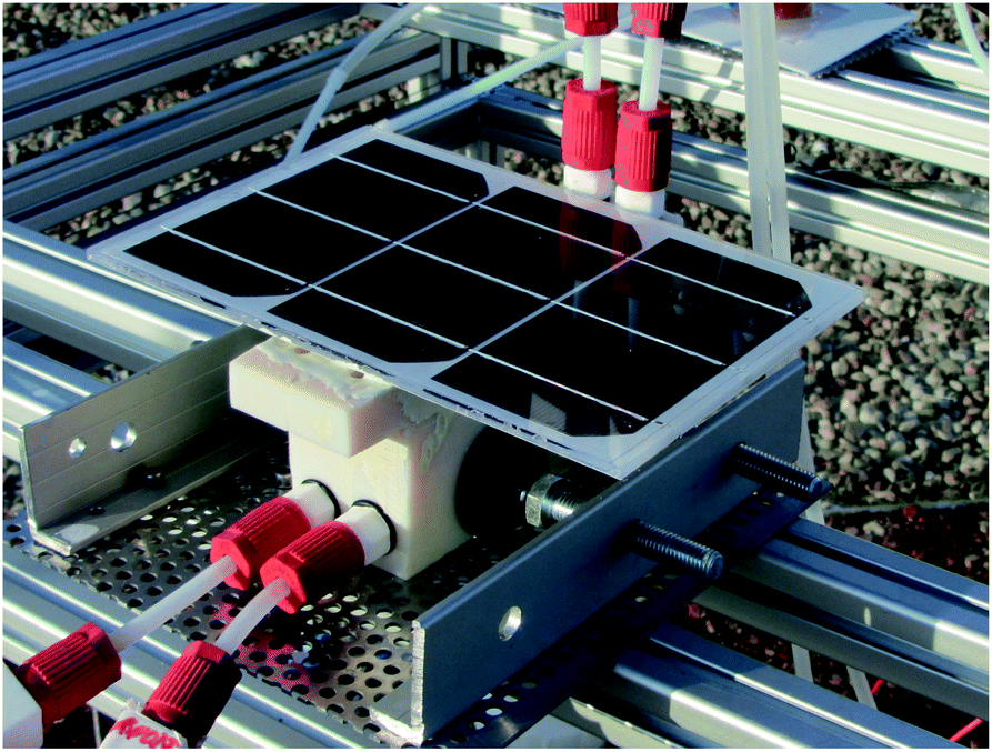 | ||
| Fig. 1 Close-up of a device similar to the analysed one (except for the different plastic used in the electrolyser casing) in the measurement setup. Electrolyte inlets at the bottom of the electrolyser, outlets at the top. | ||
The electrodes of the electrolysis component were in direct electric contact with the PV module. The electrodes consisted of 1.6 mm thick 5 cm × 10 cm nickel (Ni) foam pieces (nickel foam for battery cathode substrate, EQ-bcnf-16m, Nanografi) coated with catalysts. We used evaporated nickel molybdenum (NiMo – first 100 nm of Ni, followed by 20 nm of Mo and finally 20 nm of Ni) as the catalyst for the hydrogen evolution reaction (HER) and electrodeposited nickel iron (NiFe) for the oxygen evolution reaction (OER). During operation, the OER catalyst is most likely in an oxidized state as oxide, oxyhydroxide, or hydroxide of the metals.32
The electrolyser casing was made up of two halves made of 3D-printed transparent plastic (Stratasys VeroClear) sandwiching a separator membrane (AGFA Zirfon PERL UTP 500) between them. The membrane area in contact with the electrolyte was about 5 cm × 10 cm, equal to the geometric electrode area, which is smaller than the solar collection area. The casing was open from its top to allow contact between the back of the PV and the electrolyte for heat exchange. Since the electrolyser design did not allow for compression of the electrodes against the membrane for a zero-gap configuration, we glued them to it from their edges with small droplets of Loctite® 9492 epoxy (Henkel). Similarly, to the casing halves, the PV module was also glued to the plastic casing to seal the electrolyser with the Loctite epoxy. Details of the material choices and design challenges are presented elsewhere.33
2.2. PV and electrochemical characterization
We used laboratory tests to qualify the performance of the electrocatalysts and that of the PV module before integrating them into a single unit. The PV module was tested using a class AAA flasher (h.a.l.m, Germany) under standard test conditions (AM 1.5, 1000 W m−2, device temperature of 25 °C). The reaction kinetics of the catalyst coated electrodes and bare nickel foams were tested in 1.0 mol l−1 (1.0 M) aqueous potassium hydroxide (KOH) held at 25 °C in both 3-electrode and 2-electrode configurations. The performance data of the PV and electrodes is presented in Section 3.1 and in ESI.†2.3. Performance characterization
The IPE was characterized both indoors in a solar simulator and outdoors on a rooftop in Berlin, Germany (52°25′ 53.3′′ N, 13° 31′25.9′′ E). The outdoor characterization was performed in several measurement campaigns starting from July 2019 and continuing until the end of October 2019. One of the main aims of the measurements was to characterize the device in varying operating conditions, which in practice meant that measurements were done on sunny days with different forecasted maximum temperatures. Some overlap between the conditions on different days happened, but we tried to minimize it to maximize the spread of tested conditions, while minimizing degradation during measurements.Later in 2019 a large-area (up to 55 cm × 55 cm), LED-based continuous illumination solar simulator (Wavelabs LS-4, Germany) became available to us. We then used it for indoor measurements with the prototype to determine its performance under 1000 W m−2 irradiance, as irradiances higher than ca. 870 W m−2 were missing from the outdoor data. The spectral match classification of the simulator is class A. The homogeneity classification depends on the illuminated area, but for the area of the prototype (ca. 14 cm × 21 cm) the non-uniformity was about 1.6–1.8%, corresponding to class A. The distance between the LEDs and the PV was determined at 1000 W m−2 irradiance with a calibration PV cell, and in measurements the centre of the PV module was at the location of the calibration cell.
Except for some minor differences, the outdoor and indoor procedures were identical. Before the start of an outdoor measurement, the PV was covered so that it would not generate electric power and no gas would be produced. The time, when the cover was removed was recorded and the gas flows and temperatures were measured continuously until the end of the measurement. At the end, the PV was covered again, and to measure the total produced gas volumes the electrolyte circulation was continued, until no gas flow was measured. Indoors, the device was placed inside the solar simulator, but there was no need to cover the PV, because the irradiance with the LEDs turned off was so low that no gas production was observed. The duration of the illumination period was set in the controlling software, and the set irradiance, duration and measurement starting time were recorded.
The measurement and recording of the gas flows out of the anode and the cathode and the device temperature for later analysis with the weather data provided the input for our analysis of the device performance. Our analysis is based on data that corresponds to about 38 hours of operation, 35 of which outdoors, but we performed also other measurements that were not deemed useful for this analysis (e.g. device tilted from the horizontal plane). With all measurements together, the total operating time is about 75 hours.
The weather data (global horizontal irradiance, ambient temperature, wind speed, relative humidity, and ambient pressure) was taken from an outdoor PV weather station in the immediate vicinity of the measurement site. Indoors we measured the ambient temperature with a Pt 100 thermometer and used the ambient pressure from the PV weather station. Outdoors the device was placed so that the PV surface was horizontal and there would be nothing blocking the sun (in the south) and oriented so that the inlet was facing southeast to south. Fig. 2 shows the measurement setup.
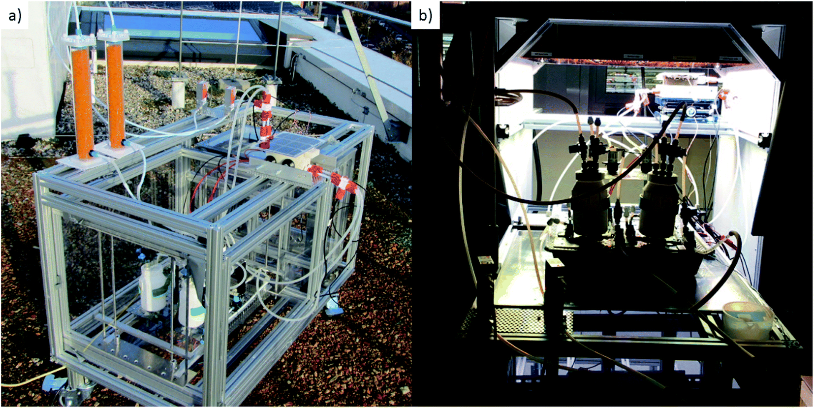 | ||
| Fig. 2 (a) The outdoor measurement setup in its latest form: the IPE on the right, the mass flow meters at back, gas dryers (orange cylinders) on the left, and pumping system, including KOH reservoirs (white PTFE flasks), at bottom. The data acquisition module was located under the mass flow meters and is not visible from this view. (b) The IPE inside the solar simulator with the rest of the test rig in the foreground. During measurements the simulator was closed with black curtains, leaving only the IPE, and the connecting hoses and the cables to temperature sensors in. | ||
During the course of the measurements, we made changes to the measurement setup, but the central parts remained the same: after exiting the electrolyser, the fluid flow entered the liquid–gas separators, also serving as electrolyte reservoirs, and the gas flow rates were then measured with Bronkhorst EL-FLOW Select mass flow meters (MFM). The temperature of the electrolyte before the inlets and after the outlets, as well as the temperature of the PV, was monitored with Pt 100 thermometers, the ones measuring the electrolyte covered with fluorinated ethylene propylene (FEP) for corrosion protection. In outdoor measurements the PV temperature was measured at the glass surface for comparability with thermography recordings that we took during some outdoor measurements. Indoors the thermometer was attached to the back of the PV at the middle of a part of the module not above the EC, because thermography recordings could not be made and the used Pt 100 attachment was large enough that it could have shaded some of the active PV area. We used 1.0 M KOH as the electrolyte, always starting a measurement with unused KOH (the electrolyte was made to circa 5.3 weight-percent KOH, which corresponds to 1.0 M concentration at 25 °C (ref. 34–36)). The electrolyte was pumped through both electrolyser chambers, in most cases at a rate of 45 ml min−1 (indoors 50 ml min−1). The anode and cathode circulations were separate, were not mixed, and both had their own pump. The volume of the electrode chambers was ca. 50 ml each and we used in total ca. 400 ml (200 ml per electrode) of KOH in measurements. Due to performance degradation of the original pumps, we had to change pumps a few times, and the 45 ml min−1 rate was chosen at one point, because it was the lowest rate that both available pumps could provide. The gas flow and temperature data (with timestamps to synchronize them later with the weather data) were recorded using a data acquisition controller module (CRIO-9047, National Instruments), on which an in-house developed LabVIEW program was running. Before each measurement campaign, the system was tested for hydrogen leaks with a handheld sensor (Sewerin Snooper Mini) and plugged if necessary.
The molar amounts of gases were estimated with the ideal gas law, using the ambient pressure from the weather data and the measured electrolyte temperatures at the outlets. The mass flow of hydrogen (g h−1 m−2) was calculated as
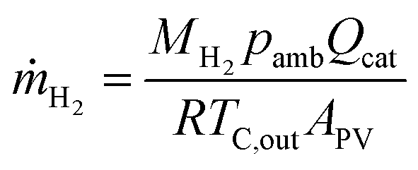 | (1) |
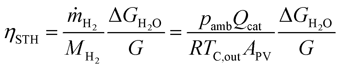 | (2) |
During some outdoor measurements, we recorded the surface temperature distribution of the PV with an infrared thermal camera (FLIR A6700SC), and analysed it using FLIR ResearchIR program. The calibration and measurements were carried out following procedures described by Usamentiaga et al.38 We used the reflector method for the reflective temperature and the reference emissivity method to determine the emissivity of the PV glass (0.983).38,39 As the reference material we used a piece of black plastic tape (Scotch™ Brand 88), with known emissivity ε = 0.96, and recommended by the camera manufacturer (FLIR).40 Here one temperature recording serves only as illustration of the temperature distribution on PV surface, and we exclude the analysis of the temperature distributions from this study.
3. Results
3.1. Performance of device components
The IV curve of the PV module measured at STC is presented in Fig. 3a while the polarisation curve of the catalysts in two-electrode configuration (electrode size 10 cm × 10 cm) in a beaker in 1.0 M KOH at 25 °C without a gas separator is shown in Fig. 3b. The individual reaction kinetics of the HER and the OER in 1.0 M KOH at 25 °C with Hg/HgO as the reference electrode (+0.927 V vs. RHE at 25 °C (ref. 41 and 42)) are shown in the ESI.†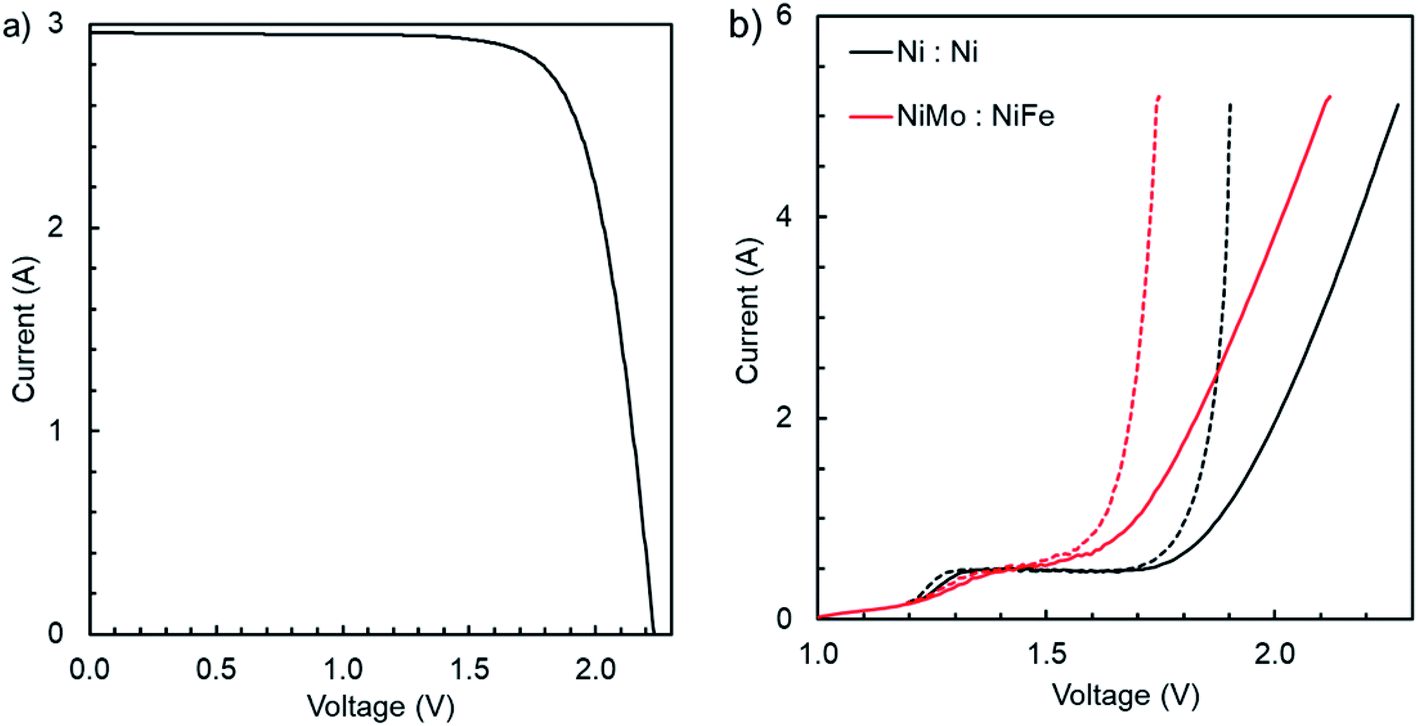 | ||
| Fig. 3 The IV characteristics (a) of the silicon heterojunction module taken at STC 1000 W m−2 and device temperature of 25 °C. The measured electrochemical performance for water electrolysis in 1.0 M KOH at 25 °C (b) using 10 cm × 10 cm electrodes in two-electrode configuration, either plain (black) or catalyst covered Ni foam (red). The data as measured is marked with solid, and 100% IR compensated with dashed lines. | ||
The short circuit and maximum power point (MPP) currents of the PV module are 2.96 A and 2.73 A, respectively, which would correspond to circa 12.4% and 11.5% STH efficiencies, if converted to hydrogen without losses. The MPP voltage is 1.83 V. Based on earlier measurements with a similar module, the short circuit- and MPP-current, and the MPP power all increase almost linearly with irradiance (see ESI†), corresponding to nearly irradiance-independent efficiency of the PV and maximum efficiency of the PV-electrolyser. The maximum power decreases with increasing temperature (due to decreased voltage), but the short circuit and MPP currents remain nearly constant (at 25–80 °C), although the MPP current decreases and short circuit current increases a little.
Turning to the electrolyser, both NiMo and NiFe catalysts show a circa 50–70 mV improvement over plain Ni, depending on the current density (see ESI†). Fig. 3b shows the performance of the catalysts compared to plain Ni foam in two-electrode configuration (1.0 M KOH at 25 °C, measured at 2 mV s−1 sweep rate). Note that in this case the electrode area is twice the size of the electrodes of the electrolyser. The comparison to plain Ni indicates a roughly constant improvement of about 160 mV, slightly higher than the 3-electrode measurements indicate. This could be due e.g. to oxidation of the 10 cm × 10 cm plain Ni foams during storage before measurements, and differences in the electrodeposition of NiFe due to different substrate sizes. The 10 cm × 10 cm electrodes were used as such both in deposition and in IV measurements, but the smaller samples for 3-electrode measurements were cut from a 5 cm × 5 cm substrate. The electrodes for the device were cut from 10 cm × 10 cm pieces, so the 2-electrode data would be more representative, if the substrate size had any significant effects on the electrodeposited catalyst. Considering the IV curve after the compensation for resistive losses (0.072 Ω, 100% compensation in both cases), 2.0 A current, equivalent to 1.0 A in the complete device, would require at least 1.68 V, and 5.0 A (equivalent to 2.5 A) 1.74 V. Compared to literature, the performance is similar to the state of the art with similar materials in the same conditions, which in turn is apparently as good as Pt and IrOx.43 For the integrated device this means that the resistive losses should not exceed 30 mΩ for the MPP operation to be achievable (the MPP voltage is about 80–90 mV higher than the minimum voltage needed for the MPP current, 2.73 A, at 25 °C). This is a rather small margin and our simulations indicate that the losses in the electrolyser alone could be higher (ESI†). In practice, this could mean that the electrodes should be a little larger or the catalysts more active to reach MPP operation in real operating conditions. Moreover, for the best results, the sizing should be done to correspond to the operating conditions, or at least for a higher temperature than 25 °C, but we were limited by our already existing design and could not fully tailor the electrolyser to the PV module.13,44 Therefore, although the catalyst performance appears promising, this should be considered more as a description of the device components than as a reasoning for the device configuration.
3.2. Results of indoor and outdoor measurements
In this section we show examples of the data collected when the device was operating continuously, one outdoors and one indoors. The transients already show some trends in the effect of temperature and irradiance on the operation, which will become clearer in the detailed analysis in Section 3.3. These are not the only measurements that we performed, but they illustrate continuous operation and effects of irradiance and temperature well. The other measurement transients considered in this analysis are shown in the ESI.†Due to pumping, the gas flow transients were noisy compared to the other transients and had to be averaged over a period of time to obtain a signal that is reasonably easy to follow. For the transient lines, we used the average over the previous 60 seconds, and the symbols represent the average over the previous 5 minutes (±1 second) that are then used in the later scatter plots and analysis. Due to the different averaging periods, the symbols do not always coincide with the 60 s average transient. Other transients (irradiance, temperatures) are as measured (at least 1 point/second). The STH efficiency was calculated from the cathode outflow, measured outlet temperature and ambient pressure, using the ideal gas law, and assuming that the cathode outflow was pure H2 (eqn (2)).
For the clarity of the transient figures, the STH efficiency is not plotted in them, but it can be estimated from the hydrogen outflow and irradiance. For example, with the collection area of 294 cm2, under 1000 W m−2 irradiance hydrogen outflow of 10 ml min−1 would correspond to about 5.6% STH efficiency (depending on the exact temperature and pressure). In Fig. 5 the hydrogen outflow transient overlapping with the irradiance corresponds to about 8.4% STH efficiency, in Fig. 6 to about 5.3%.
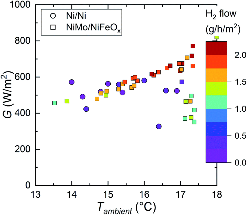 | ||
| Fig. 4 Comparison of the current (squares) and earlier prototype (circles): hydrogen generation rates measured under similar outdoor conditions as a function of irradiance and ambient temperature. | ||
We simulated the operation of the electrolyser with COMSOL® Multiphysics software to understand its operation and to find effective ways to improve its performance. The simulations mainly focused on the effects of different geometric features on the electrolyser performance (more details in the ESI†). Minimizing the electrode separation was expectedly an important change, as well as minimizing the electrolyte volume. The optimal thickness of the porous electrode depends on the balance of mass transport and reaction kinetics, and therefore on the current density. In our case, it seemed that near the MPP of the PV module the electrode thickness might not have a significant effect. Therefore, for simplicity and because (due to neglecting gas bubbles) it was considered more likely that the simulations would underestimate rather than overestimate mass transport losses, the electrode thickness was reduced to a single Ni foam piece (1.6 mm). The possible improvements from reduced electrolyte volume have not yet been implemented in the current prototype due to time constraints.
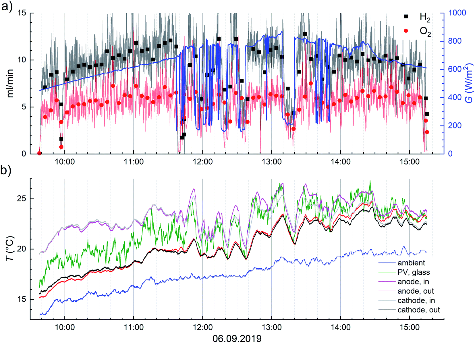 | ||
| Fig. 5 Time dependent profiles measured on 6th September 2019 in Berlin, Germany of (a) H2 and O2 flow rates and solar irradiance transients. Flow rate transients are averaged over 60 seconds (lines) and 5 minutes (squares and circles) to reduce noise in the signal. (b) Time dependent profiles measured on 6th September 2019 of ambient, PV glass and electrolyte temperatures. | ||
The dip in gas production rate at 09:55 was due to an interruption while recording the PV surface temperature distribution (shown in Fig. S4.10†) with the infrared camera before starting a new continuous measurement. There were also short interruptions in the outdoor monitoring data in Fig. 5, due to small electrolyte leaks at the inlet ports at about 11:40 and 12:50 that can be seen when carefully looking at the gas flow transients.
We did not study the sensitivity of hydrogen generation to partial shading of the PV module, but we believe that it is more sensitive to shading than electric power generation with PV modules due to the minimum required voltage for the electrolysis reaction. The series connection means that in the case of shading, hydrogen production is always limited by the lowest photocurrent and the affected area is tripled compared to a single cell. For electric power generation, bypass diodes in modules reduce the power losses (and damage to cells) due to shading, but the MPP voltage is still reduced. The voltage requirement of the electrolysis reaction means that the effects of even partial shading will directly affect the EC operation due to direct coupling, reducing hydrogen generation rate in proportion to the shaded area or even completely stopping it, if the photovoltage is sufficiently reduced. In this comparison, electricity generation benefits from the flexibility regarding the photovoltage compared to the almost fixed minimum voltage of the EC. With a single multi-junction PV cell driving an EC, the sensitivity could be reduced compared to multiple series-connected PV cells, but probably still higher than for electricity generation due to the minimum voltage of the EC.
In almost all the measurements, the outlet temperatures were cooler than the inlet temperatures, suggesting that heat was lost to the environment from the electrolyser. This is most likely due to the electrolyte reservoirs being exposed to sunlight and being heated by it, while the PV covered and shaded the EC (see Fig. 1 and 2), and due to ineffective heat conduction from the PV to the electrolyte, most likely due to gas pockets formed at the top of the electrode chambers. Admittedly, the PV glass temperature was not much higher than the electrolyte temperatures, but from the thermographic images (such as the one shown in Fig. S4.10†), we noticed that the measured spot was typically a few degrees cooler than the highest temperature. Therefore, the real temperature of the PV, especially the silicon itself, was most likely a few degrees hotter than the transients at all times. Consequently, the temperature gradient between the PV and the electrolyte was also higher, favouring heat transfer from PV to electrolyte. However, as the transients show, heat transfer was not efficient enough to even maintain the inlet temperature. We consider the gas pockets that we observed to be formed at the top of the electrode chambers (between the liquid electrolyte and the back of the PV) the most likely reason for the thermal insulation of the electrolyte from the PV.
The measurement setup was developed continuously and improved over time. Leaks and other difficulties during the first measurements prevented unsupervised operation of the device for long time periods. Therefore, measuring continuous operation for longer than few hours was not possible in practice. Developments to the electrolyte pumping system and plumbing significantly reduced the leakage problems, so that we could test the device operating overnight, but only in the autumn when the irradiation was significantly lower and days shorter than in the summer. The transients from this measurement on 22nd to 24th October 2019 are shown in the ESI (Fig. S4.6–S4.8†).
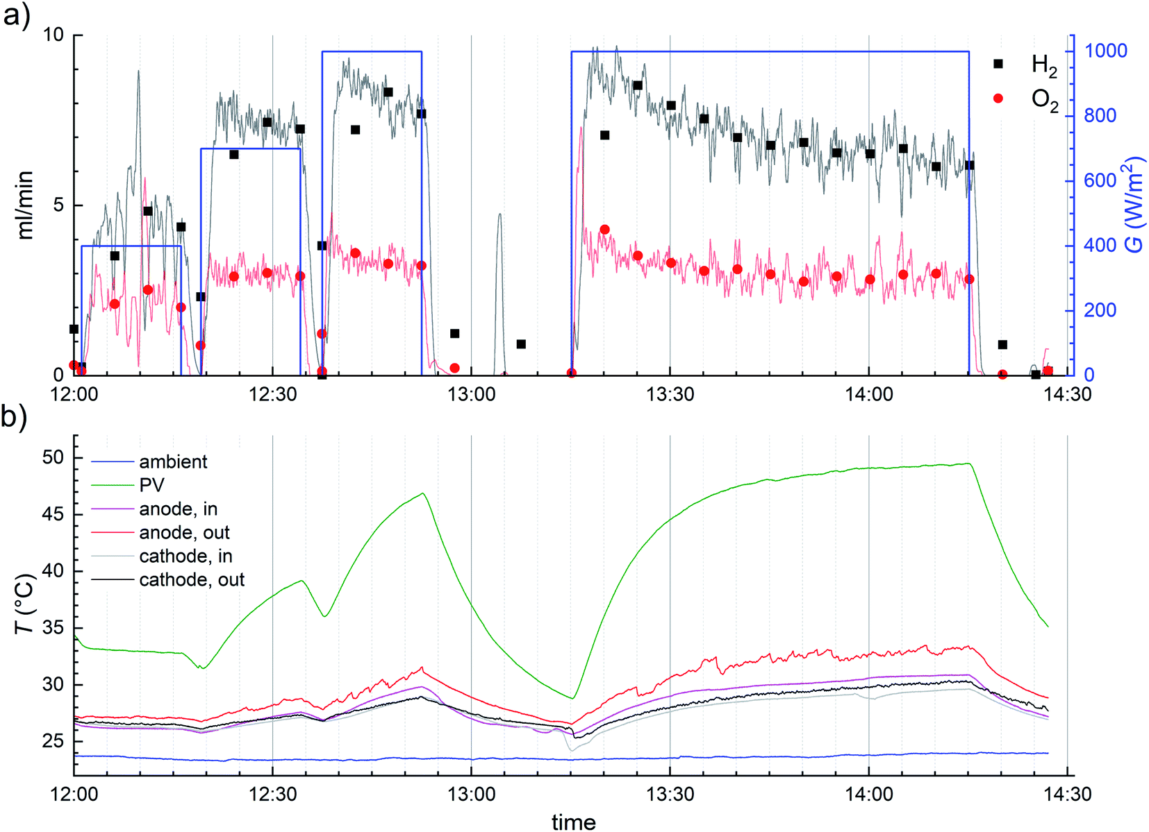 | ||
| Fig. 6 Time dependent profiles measured indoors of (a) H2 and O2 flow rates and solar irradiance transients. Flow rate transients are averaged over 60 seconds (lines) and 5 minutes (squares and circles) to reduce noise in the signal. (b) Time dependent profiles of ambient, PV and electrolyte temperatures. | ||
Especially the 1 hour measurement starting from 13:15 illustrates well the importance of the PV temperature. Initially, with a relatively cool PV (ca. 35 °C) the hydrogen outflow reached a peak level of 9–10 ml min−1, corresponding to about 5% STH efficiency, but as the PV temperature increased, the gas production rate decreased. At the end of the 1 hour measurement the temperature was steady, at nearly 50 °C, and the gas production rate about 6 ml min−1, corresponding to an STH efficiency of about 3.5%. After the illumination was turned off, the electrolysis reactions stopped, and the gas outflow decreased fast, as the remaining gases were flushed out of the EC. As the irradiance no longer heated up the device, the temperature began to cool as well. To a lesser extent the same can be observed in nearly all indoor transients.
During the indoor measurements, the electrolyte temperature was monitored and not actively controlled. Because only a small part of the electrolyte tubing was under irradiation in the solar simulator, the increase of the electrolyte temperature over time suggests that some heat may have been transferred from the PV after all. However, as the temperature difference became large with the PV heating up, the transfer was probably not effective.
3.3. Effect of temperature and irradiance on the device operation
The most important factors affecting the device operation are the solar irradiance, i.e. input power, and the ambient temperature, which affects the operating temperatures of the PV and electrolyser and therefore their IV characteristics. The efficiency of the SHJ PV-module was expected to be nearly independent of irradiance (at constant operating temperature). However, because the operating point of an IPE device is not at the MPP of the PV, but determined by the IV-matching of the PV module and electrolyser, the STH efficiency is not necessarily independent of irradiance. Based on literature, the STH efficiency can decrease significantly with increasing irradiance, but it could also remain (nearly) constant, even when the electrolyser is not well-matched to the PV.8,44,45 Nevertheless, increased temperature reduces the voltage of both the PV and the electrolyser. In principle, the performance of the integrated device could then be both improved and reduced, the net effect depending on whether the electrolyser or the PV voltage is reduced more.In this section we focus on the relationship between the measured performance (hydrogen production rate and STH efficiency) and the operating conditions (both the device and the ambient temperature, and the irradiance). In addition, we discuss the irradiation spectrum, and gas crossover and its implications for the efficiency characterization and device safety. The points in the scatter plots correspond to the 5 minute averages of the transients during continuous operation, with low-irradiance (less than 100 W m−2) points excluded from the discussion.
To determine the validity of using only the irradiance as the descriptor of the outdoor data, we extracted the following spectra measured in sunny conditions: the time point closest to one of the highest irradiances in our data (840 W m−2 at 13:05 on 6th September 2019, see also Fig. 5), the highest H2 generation rate at less than 750 W m−2 (2.1 g h−1 m−2 at 678 W m−2, 11:32 also on 6th September 2019) and the range of about 200–550 W m−2 (on 22nd September 2019, apparently cloudless afternoon – transients in Fig. S4.4 in ESI†). We had only the spectra measured at 35° tilt facing south available to us, so the spectral shape could differ a little from the irradiance at the horizontal plane. Because the spectrum was measured once every 5 minutes, we often had to choose the spectrum closest to the relevant point in time or a round number irradiance. Naturally, when the intensity reduction is due to clouds, it is not expected that the shape of the spectrum would match clear sky conditions, but we did our measurements in mostly sunny conditions, so we exclude other conditions from this discussion. Also, because we excluded low irradiance (<100 W m−2) data points from the results, any measurement in overcast conditions would have been consequently excluded.
The irradiance spectrum of the solar simulator was measured with a spectroradiometer (Instrument Systems CAS 140CT with ISP40 optical head connected with an optical fibre). The relative irradiance spectra are shown in Fig. 7 in comparison with the AM1.5G standard spectrum. As a difference to the others, the solar simulator spectrum is normalized so that 1 corresponds to the maximum irradiance of the AM1.5G spectrum, not to the maximum irradiance of the spectrum in question.
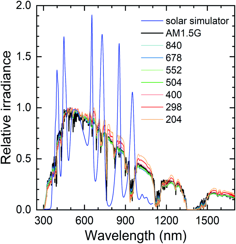 | ||
| Fig. 7 Relative irradiance spectra of the solar simulator and for irradiances (W m−2 at horizontal plane) in sunny conditions ranging from about 200 W m−2 to 840 W m−2 compared with AM1.5G. Data were collected on 6th September 2019 (678 and 840 W m−2) and on 22nd September 2019 (204–552 W m−2) in Berlin, Germany at a 35° tilt from the horizontal plane. Solar simulator spectrum is normalized so that 1 corresponds to the maximum irradiance of the AM1.5G. | ||
As expected, at low irradiances the spectral shape differs from the standard spectrum at longer wavelengths due to atmospheric scattering. In principle, the increased long-wavelength irradiance could enhance the PV performance by increasing current (and voltage) and reducing heat generation compared to the AM1.5G. Also, depending on the EQE spectrum, the peaks in the simulator spectrum could have a disproportionate effect on the PV operation. However, in all cases the spectral mismatch is small enough that they would be classified as class A solar simulators. Therefore, and because the EQE spectrum of our PV cells should be nearly constant in the wavelength range with the variations, the spectral differences in outdoor measurements, or even the peaks in the solar simulator spectrum, should not have significant effects on the PV performance.31 As we could only access the spectra at a tilted plane, there could be minor differences to the horizontal plane. Nevertheless, it seems safe to assume that the spectral shape is not a significant factor for our data, so the irradiance alone should describe the operating conditions sufficiently accurately (together with the ambient temperature).
The STH efficiencies were calculated from the average H2 generation rates, and temperature and irradiance are also 5 minute averages. The fastest change in outlet temperature was the ca. 3 °C drop in about 10 minutes at 13.10–13.20 on 6.9.2019 (Fig. 5.) and in PV temperature about 5 °C increase in 5 minutes, as the solar simulator was turned on to 1000 W m−2 (Fig. 6 and S4.9†). Some similar PV temperature changes occurred also outdoors, but most changes were slower, so the effect of outlet temperature on H2 flow and STH efficiency is less than about 0.3% (relative) and the PV temperature error is at most about 2.5 °C, but in most cases significantly less. The delay in the gas outflow after irradiance changes, when they happened, had much larger impact on the averaged performance.
The recorded H2 generation rates and calculated STH efficiencies as a function of the PV temperature and irradiance are shown in Fig. 8. The outdoor measurements are marked with squares and indoors measurements with stars. The generation rate clearly increases with irradiance, and the highest rate was achieved with a cool PV under comparatively high irradiance. The STH efficiency seems relatively independent of the irradiance and appears to decrease with increasing temperature. The outdoor points with the highest performance at 18–24 °C PV temperature and irradiance over 450 W m−2 were measured on 6th September (Fig. 5), which was the last outdoor measurement with irradiance over 600 W m−2 for extended times. Therefore, the STH efficiency reducing with increasing temperature at high irradiances is certainly not a degradation artefact. Plotting the STH efficiency against the temperature provides a more detailed picture of the situation, indicating that the temperature is significantly more important to the STH efficiency than the irradiance (Fig. S5.1† and 9).
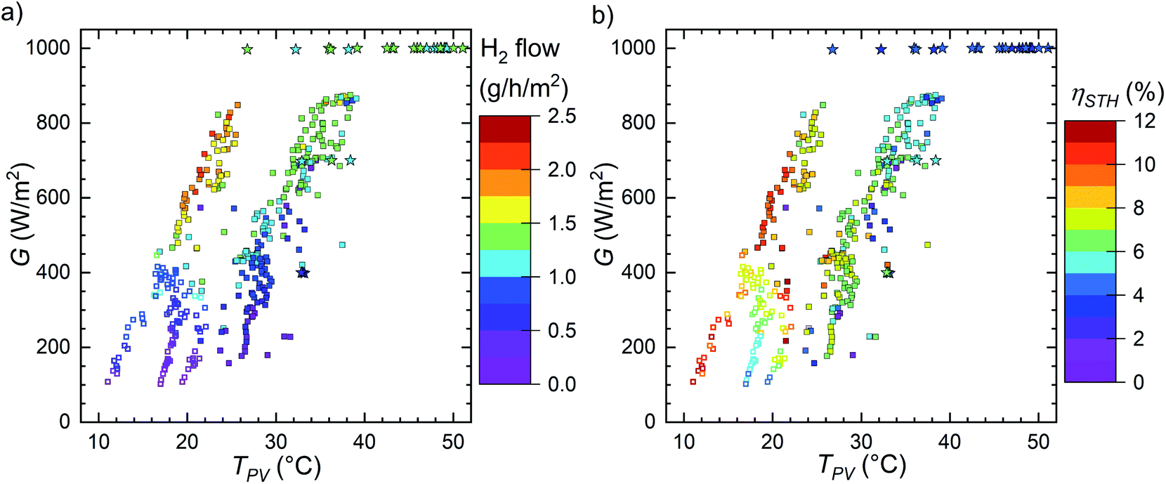 | ||
| Fig. 8 (a) The H2 generation rate and (b) the STH efficiencies as the function of the measured temperature of the PV and the irradiance. The values are a consolidation of indoor and several outdoor measurement campaigns on various days with a variety of weather conditions. Outdoor data (front glass) marked with squares, indoor data (back of the PV) with stars, open squares indicate the measurement on 22 to 24.10.2019 (Fig. S4.6–S4.8†). | ||
 | ||
| Fig. 9 The solar to hydrogen conversion efficiency, ηSTH as a function of the ambient temperature, divided into groups of different irradiances. Outdoor data marked with squares (open squares 22 to 24.10.2019), indoor data with stars. The dashed line indicates a −0.35% °C−1 slope. | ||
The last outdoor measurement (on 22 to 24.10.2019, Fig. S4.6–S4.8†) seems slightly different from the pattern of the other outdoor measurement, which is best seen in the STH efficiency. The open squares in Fig. 8–11 correspond to this measurement to differentiate it from the other outdoor data. Compared to other outdoor measurements, these points in Fig. 8b seem as if they were shifted to about 5–10 °C cooler temperatures, i.e. the STH efficiency is lower than previously at the same temperature. Based on Fig. 9 and S5.1,† it also seems possible that in this case the efficiency decreases faster than earlier with increasing temperature. At first, the H2 generation rate may seem to match the previous outdoor measurements, but there is an abrupt jump from less than 1.0 g h−1 m−2 to more than 1.5 g h−1 m−2 at 450–500 W m−2 and ca. 18 °C (or ca. 15 °C ambient, see also Fig. 11 and S5.2†) and few older points hint to a significantly higher performance in the same conditions. Since this is one of the last measurements we did, the difference could be due to degradation. The indoor measurements were performed after all outdoor measurements, but due to higher PV temperatures, directly comparing them to outdoor measurements is unfortunately difficult.
If the last outdoor measurement is excluded, the temperature dependence of the other points is about −0.23% °C−1 (absolute change in the STH efficiency, see Fig. S5.1†). This is clearly steeper than the −0.044% °C−1 (absolute) efficiency coefficient determined earlier for a PV module similar to the one used in the device (see Fig. S1.6†), meaning that the operating temperature of a PV-EC device seems to be more important than the temperature of PV modules, which could have implications to the design and operation of PV-EC devices. The operating point of the PV-electrolyser being at a higher voltage than the MPP of the PV could contribute to this, by the electrolyser IV-curve magnifying the effect of the voltage reduction on the operating current. Because the outdoor points fit the trend regardless of the irradiance, it seemed plausible that this was genuinely a temperature effect and not a combined effect of both the temperature and irradiance.
There were clearly fewer data points indoors and their irradiance range was narrower. The gap in Fig. 8 makes the comparison difficult, but their STH efficiency appears to match the general pattern and trend of the outdoor measurements (Fig. S5.1†). The efficiency in solar simulator under 1000 W m−2 ranged about 3.4–4.9%, depending on the PV temperature. These values are lower than most outdoor data most likely due to hotter PV and in some cases also cooler electrolyte. Also, the values at the lowest PV temperatures for a given irradiance are most likely underestimated, because they include the ramp up phase of the gas production (see Fig. 6 and S4.9†).
Due to weather conditions and device heating indoors we could not test our device in the standard PV testing conditions (STC), i.e. 1000 W m−2 and 25 °C PV temperature. However, if the outdoor and indoor measurements describe the same trend, then the outdoor values at 25 °C PV temperature indicate approximately 7–8% STH efficiency.
Naturally, the different locations of the thermometer indoors and outdoors meant that the measured temperatures were not completely the same. However, based on outdoor measurements, during which PV temperature was recorded for both the front and the back of the PV, we do not expect the back of the PV to be more than a few °C warmer than the front (temperature measurement for the back of the PV was carried out for only few outdoor measurements, since the number of recorded sensors was limited and initially the EC casing temperature was recorded instead). Therefore, we are not certain that the match between indoor and outdoor measurements is quite as seamless as especially Fig. S5.1† indicates, and some caution is advised in their comparison.
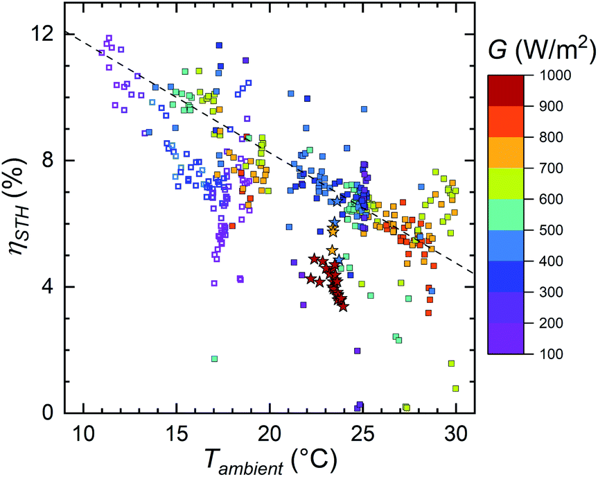
The STH efficiency as a function of the ambient temperature is shown in Fig. 9 (for hydrogen outflow see Fig. S5.2† and 11). The trend of the outdoor measurements is almost the same as it was with the PV temperature, only the slope changes due to the change in temperatures. Except for the different slope, the only difference is that few points at circa 29 °C ambient and 600–800 W m−2 irradiance now deviate from the general trend. The most likely reason is that, for some reason, during the corresponding measurement the EC temperature was higher than the PV temperature (29th August, Fig. S4.3†). As we observed this only once, the PV being cooler than the electrolyser seems more of a rare exception than a typical operating mode of the device.
The indoor measurement points now indicate significantly worse performance than the outdoor measurements at the same ambient temperature. Still, the indoor STH efficiency would be at a similar level as the last outdoor measurement, if the temperature dependency was similar to the earlier measurements. Most likely the performance had degraded somewhat and the PV temperature could have been underestimated outdoors, but we are uncertain of how much they affect the data. Wind cooling the PV significantly more than natural convection indoors would also explain the difference between Fig. 9 and S5.1† (and between Fig. 8 and S5.2†), but it would have to correspond to about 10 °C temperature difference. While not impossible, low wind speeds would explain roughly half of that, leaving the rest of the difference to degradation, PV temperature measurement differences and possible other factors.51 Additionally, due to the PV heating up during the indoor measurements, some points at practically the same ambient temperature correspond to clearly different PV temperatures, and the efficiency spread is a little larger than in the outdoor measurements.
If all outdoor measurements with the electrolyser at the same or a cooler temperature than the PV glass are considered, excluding the last measurement on 22 to 24.10.2019, the points form a line, whose slope is approximately −0.35% °C−1 (absolute, the dashed line in Fig. 9), even steeper than the PV temperature slope. The STH efficiency as a function of ambient temperature would be accurately represented also by an exponential decrease (ESI Fig. S5.3†) that would reduce the H2 generation rate by about 1% (relative) per 0.25 °C increase in temperature.
Combining the effects of the irradiance and the ambient temperature on the H2 production rate outdoors, using 25 °C as a reference temperature gives
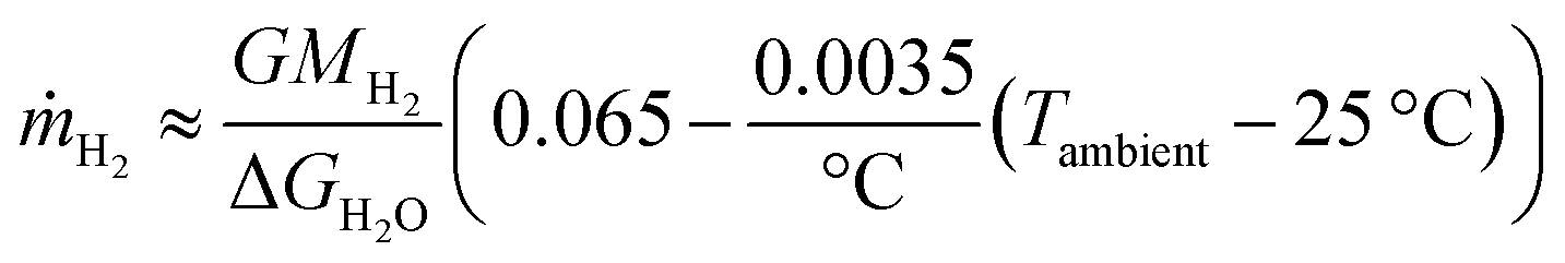 | (3) |
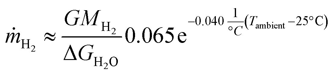 | (4) |
Similarly to eqn (1), the irradiance, Gibbs free energy, and molar mass of H2 are G, ΔGH2O, and MH2, respectively. These trends are plotted with a dashed line in Fig. 9 (eqn (3)) and S5.3 (eqn (4)).† While the accuracy of these formulas outside the tested range of conditions is uncertain, some limits and criteria can be established. The short circuit current of the PV limits the STH efficiency to less than 12.4%, which the linear formula would match at 8.1 °C and the exponential decrease at 8.8 °C, so measurements at 10 °C and cooler could have been useful. An additional limit is that the linear formula predicts that at 43.6 °C no hydrogen would be produced, whereas the exponential decrease yields about 3.1% STH efficiency at this temperature. Naturally, if the results from the last outdoor measurement were not due to degradation, but caused by the normal response of the device to the operating conditions, they would increase the spread in the data. The ambient (or PV) temperature would no longer describe the performance quite as accurately, and other factors would have to be considered, most likely including irradiance.
Considering that the efficiency of the device depends on its H2 generation rate, i.e. operating current or crossing point of the PV and EC IV-curves, it is admittedly surprising that the irradiance would have no effect on the STH efficiency, despite some literature examples indicating such a possibility.14,44 Almost all STH efficiency points in the previous figures were below the MPP current value (ca. 11.5%), so our device was clearly operating at a higher voltage and a lower current, indicating too high voltage losses in the electrolyser. Therefore, the crossing point would have been expected to be sensitive to the operating conditions, meaning that the STH efficiency could have depended also on the irradiance in addition to temperature. However, a small effect could have been also hidden underneath the scatter in the data. Determining the temperature-dependency of the electrolyser IV characteristics would be a key part to answering this problem.
While testing the device stability was not one of the main goals of our study, degradation in the last outdoor measurement would indicate a quite sudden performance drop after about 55 hours of operation under natural sunlight, as the previous measurement seemed to match the STH trend of the earlier measurements (400–600 W m−2 at 20–25 °C ambient, transient shown in Fig. S4.5†). More testing would be needed to determine the possible performance drop and its causes, but so far, the device has been tested for about 75 hours under real and artificial sunlight and it remains operational.
![[thin space (1/6-em)]](https://www.rsc.org/images/entities/char_2009.gif) :O2 ratio of the electrolysis reaction. Using our handheld hydrogen detector, we quite commonly observed small amounts of hydrogen in the anodic outflow, and significant hydrogen crossover and/or leakage to the outside should result in the outflow ratio being less than 2.0.
:O2 ratio of the electrolysis reaction. Using our handheld hydrogen detector, we quite commonly observed small amounts of hydrogen in the anodic outflow, and significant hydrogen crossover and/or leakage to the outside should result in the outflow ratio being less than 2.0.
For alkaline electrolysis, the most important cross over mechanisms are differential pressure over the separator, mixing of anolyte and catholyte with each other, and diffusion of dissolved H2 and O2 molecules through the separator.52 Because we never mixed the anolyte and catholyte, this can be excluded from the discussion. Because more H2 is produced than O2, and H2 is smaller and more mobile than O2, the amount of H2 in O2 is normally higher than the amount of O2 in H2.52–54 Therefore, the concentration of H2 in the anodic outflow is the main crossover descriptor, and the ratio of the cathodic outflow to the anodic outflow would have been expected to be less than 2.0, regardless of the current density. However, at low outflow rates our measurements yielded ratios higher than 2.0, which seemingly contradicts the literature (Fig. 10), at first suggesting O2 crossing to the catholyte. Due to the intermittency of the operation and the lack of voltage control of the electrolyser, even fuel cell reactions and reactions with catalysts could contribute to this situation.55
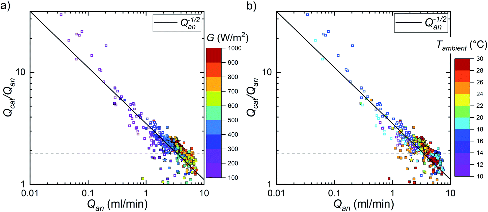 | ||
| Fig. 10 Ratio of the cathodic outflow to the anodic outflow as a function of the anodic outflow, grouped according to (a) irradiance, and (b) ambient temperature. Outdoor measurement points are marked with solid squares (open squares 22 to 24.10.2019), indoor with stars. The dashed horizontal lines mark the ratio 1.88, which corresponds to the lower explosive limit of H2 (4%). | ||
The 5 minute averages of the volume outflows as a function of the anodic outflow are shown in Fig. 10. Because the indoor markers are mostly covered by the outdoor markers, it does not really show, but the indoor measurements conform to the trend of the outdoor measurements. Using the cathodic outflow as the comparison produced more scatter in the data at low outflows and lower ratios than the anodic outflow (see ESI, Fig. S5.4†). The ratio was the highest, significantly higher than 2.0, at low gas production rates and reduced when gas production increased. However, as a minor difference, when plotted against the cathodic outflow, the ratio increased slightly at high outflow, suggesting that overall low operating current densities could be a part of the problem. At the highest anodic outflows, the ratio was generally less than 2.0, indicating possible H2 crossover to the anode side. Therefore, because it is obvious that the outflows are not necessarily pure hydrogen or oxygen, we discuss them here as the cathodic and anodic outflows.
In principle, leaks out of the system could be possible, but we tested the system for hydrogen leaks at the beginning of every measurement with a leak detector and stopped the measurement for repairs, if a leak was detected. On the other hand, the ratio being higher than 2.0 implies that oxygen could have been lost in some process. As Fig. 10 shows, it seemed that the ratio followed a power law dependence close to 1/Q1/2, which may be specific to our device. As far as we could tell, temperature and irradiance had no clear effect on the outflow ratio, except for their effect on the gas generation and outflow rates (see also Fig. S5.5†). In Fig. 10a the irradiance groups are mostly organized to colour bands, outflow increasing with irradiance, and in Fig. 10b the ambient temperatures are mixed with each other. Most of the values below circa 3 ml min−1 and ratio higher than 2.0, originated from the last few outdoor measurements, which had a different pumping system compared to the earlier ones. Therefore, at least in principle, the ratios from these measurements could have had different factors affecting them and the low and high ratios could have been due to different phenomena. However, all the points seemed to fit a continuous trend, and this effect arising from a combination of two unrelated trends seems unlikely.
A possible hint is that at some points at low irradiances the anodic outflow was reduced to negligibly small levels, which did not happen with the cathodic outflow (Fig. 11). Considering this, and the roughly linear slope of the anodic outflow, it seems possible that a parasitic reaction consumed oxygen at a rate independent of the electrolysis rate.56 Oxygen can readily oxidize the OER catalyst (NiFe-based) at the anode working potentials, and the resulting material is likely ion-permeable oxyhydroxide, potentially enabling the reaction to penetrate into the bulk beyond the solid–liquid interface.32 Since this reaction would only need the typical anode operating conditions to proceed, it almost certainly contributes to the oxygen loss. As a slow reaction compared to OER at high overpotentials, catalyst oxidation therefore appears a likely candidate for oxygen consuming reaction that would become apparent at low irradiances, in line with the observed trend (Fig. 10, 11, S5.4, and S5.5†), and we consider it more likely than O2 crossing to catholyte.
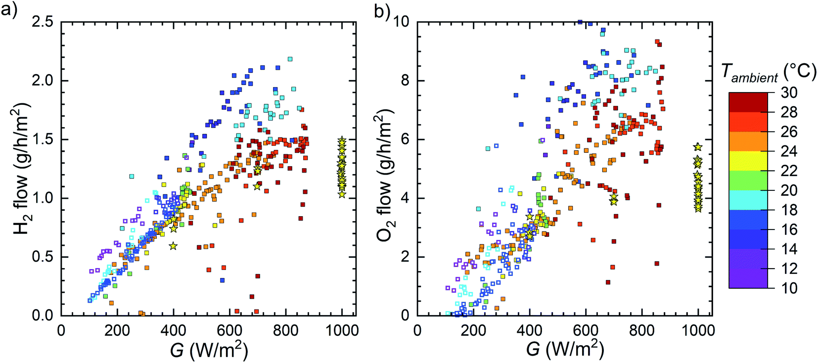 | ||
| Fig. 11 (a) The hydrogen flow rate and (b) oxygen flow rate as a function of irradiance, assuming that the outflows are pure H2 and O2. Pure H2 and O2 outflows at 2.0 H2:O2 molar ratio would correspond to 4.0 g of O2 per 1.0 g of H2. Outdoor data marked with squares (open squares 22 to 24.10.2019), indoor with stars. | ||
An alternative explanation could be that there was an irradiance threshold for the electrolysis, e.g. due to voltage limitations, and a small amount of air constantly leaked into the cathode side. We observed a leak into the cathode tubing once in a measurement excluded from these results, apparently due to a badly set fitting after the cathode outlet, but the effect on the outflow ratio was significantly more pronounced than in Fig. 10 (ratio 5–10 at 1–2 ml min−1 anodic outflow). Still, because we have noticed that a leak could affect the outflow measurement and could not determine the cathode outflow composition, we cannot completely exclude a slow leak as an explanation, but it would have had to happen at a nearly identical rate in every measurement. In practice, this would limit the location of the leak to the parts that were not changed between the measurements, i.e. directly at an inlet or an outlet of the electrolyser, or even through the epoxy joints in an extreme case. However, to have enough space for the device in the solar simulator, we changed the outlets and fittings for the solar simulator measurements, and the outflow ratios seem similar to the outdoor measurements, so this scenario seems somewhat less likely. In principle, there could have been also a bottleneck in the anode side of the circulation system and tubes creating higher pressure, when gas was produced at a low rate. However, with increased gas evolution rates, the bottleneck should have caused a smaller pressure increase than the difference of the oxygen and hydrogen partial pressures, and we are uncertain, how this would be possible, if at all.
The deviation of the outflow ratio from 2.0 naturally has implications on the STH efficiency and operation safety. When the ratio is less than 2.0, the cathode outflow is the amount of hydrogen that can be collected, so it represents the device performance the best. In the case of higher ratios, the hydrogen production rate and the STH efficiency may need to be corrected, depending on the cause of the increased ratio. In the case of parasitic oxygen consumption at the anode the cathode outflow is the amount of hydrogen that can be collected, but a slow leak to the cathode tubing would mean that the true hydrogen production rate pattern would be similar to the anodic outflow (Fig. 11b), so some low-irradiance STH efficiencies would be reduced compared to Fig. 8 and 9.
Regarding the operational safety, the lower explosive limit of 4% H2 in O2 corresponds to a ratio of 1.88, and lower ratios correspond to a higher fraction of H2 in the anodic outflow (assuming negligible O2 crossover).57 This limit is marked with horizontal dashed line in Fig. 10. Unfortunately, most ratios at anodic outflow more than 4 ml min−1 were below this limit, indicating potentially explosive mixture at the anode outflow. As an explanation for the outflow ratios higher than 2, we consider air leaks into the cathode and especially O2 consumption in a parasitic reaction more likely than O2 crossover into the cathode side. Oxygen consumption would not add any impurities into the cathode outflow, but, combined with H2 crossover, it could result in a hydrogen-rich anode outflow. An air leak into only the cathode side would naturally dilute the H2 directly in proportion to the extra volume over the 2.0 ratio, e.g. 4.0 would correspond to the flow being only 50% H2 and ratio 10 to 20% H2. Without knowing the exact cause, it is difficult say how significant concern the outflow ratios higher than 2.0 are, but in general the measured outflow ratios necessitate improvements to gas separation in our device and measurement system, and possibly changes to the way the device is operated, especially at low irradiances. Certainly, the problem(s) will have to be identified and solved, before any future commercial operation would be feasible. For a safer operation of devices, several solutions may be considered to reduce the risk of H2 concentration on the anode side increasing beyond the explosion limits. For a special case like ours, in which the photon absorbing power source and the electrolysis cell cannot be separated, the use of recombination catalysts is probably the best option and this shall be taken into consideration for future designs.52
4. Summary and discussion
We have constructed an integrated photovoltaic electrolyser with a 294 cm2 solar collection area. To aim for the optimum of high-efficiency and low-cost, we based the device on series-connected SHJ PV cells and an alkaline electrolyser with non-Pt-group based catalysts, and characterized it in solar simulator and in outdoor conditions. We can continuously measure the gas outflow from the device and the temperature of both the PV module and the electrolyte. The device has operated for circa 75 hours during different measurements, of which about 38 hours were useful for this analysis. The longest measurement lasted almost two days without problems, so we believe that our measurement system allows for even longer measurements. While 75 hour operating stability would not be remarkable, it is still quite good overall, and typical for an IPE device.11 The STH efficiency seems to mainly depend on the (ambient) temperature. The temperature dependency itself is somewhat expected, but despite literature indicating the possibility, the seeming independency on irradiance is a little surprising. The comparison of the relative irradiance spectra for a wide range of irradiances suggests that the spectral shape did not significantly affect the operation, at least in sunny conditions.Although we measured the device operation in a solar simulator under 1000 W m−2, we could not cool the PV to 25 °C during continuous operation, so the efficiency at the STC conditions is unknown. Nevertheless, with the PV heating up, the STH efficiency was about 3.4–4.9%, depending on the temperature. Outdoors, we were limited to below 870 W m−2, so the relevance of these results to higher irradiances is a little uncertain. Still, if the STH efficiency was truly independent of the irradiance, it would be 7–8% at 25 °C PV temperature, and 6–7% at 25 °C ambient temperature. Compared to other non-concentrating devices in literature, even 3.4% would be the highest reported value for a device area larger than 100 cm2, which we somewhat arbitrarily defined as the lower limit of scaled-up devices. More data on the electrolyser operation (effect of temperature, electrolyte flow etc.) and on the operation of the IPE itself (wider range of conditions) would be needed to understand why the STH efficiency seems independent of the irradiance, when this independence applies, and when it does not apply.
Our temperature range is somewhat narrow, so based only on the measured data, we cannot be certain of what kind of temperature dependency would best describe the relationship to the ambient temperature. The linear slope of the STH efficiencies from all measurements is circa −0.35% °C−1 (absolute) and the exponential reduction corresponds to about 1% (relative) reduction per 0.25 °C increase. The slope is significantly steeper than the temperature dependency of typical SHJ PV, for instance, and the decrease occurring at the typical operating conditions of the PV-EC makes it an important concern for practical operation. At colder temperatures the efficiency increase should stop at some point, because the short circuit current of the PV module limits the STH efficiency to below 12.4%. Different pumping rates in the early data could skew the results, but from comparisons within continuous measurements we know that increased temperature does reduce the gas production rate. Additionally, the temperature dependency of the STH efficiency and also the temperature difference between PV and the EC mean that a laboratory measurement at a fixed device temperature, negating the heating effect of irradiance, is not necessarily representative of the device operation in real world conditions.
Improving heat conduction from the PV to the electrolyte should reduce the temperature slope of the STH efficiency. Increasing the contact area between the EC and PC and removing the gas bubbles from the top of the EC should help to accomplish this. For the gas accumulation, reducing the distance between the outlets and the top of the EC chambers and tilting the device up from the horizontal plane are perhaps the easiest and most effective methods to reduce the problem. Additionally, flow field design, electrode morphology optimization, and faster electrolyte pumping rate (possibly at the cost of the overall system efficiency) can be helpful in this pursuit.
As we could measure only the outflow volumes, but not their composition, we were limited to the ratio of the cathodic to the anodic outflow in our analysis. The ratios below 2.0 can be explained as H2 crossing to the anode side, but the higher values require a different explanation. Although O2 consumption in OER catalyst oxidation would be a natural process that could be expected to always occur to some extent, we cannot conclusively exclude leaks from the surrounding environment as a contributing factor. Gas composition analysis could help to find the cause, because the considered options should result in a different cathode outflow composition. Because the ratio as a function of the anode outflow seems continuous, it seems possible that a continuous variation of the same physical phenomena explains both the too high and too low values. In any case, more information is needed to fully understand what caused the observed trend in the outflow ratio.
As the STH efficiency was below 11.5%, to which the MPP operation corresponded, the voltage losses in the electrolyser and electric connections have to be reduced for optimal operation. The electrodes could be larger, but we probably cannot increase their size enough that the reduction in the kinetic overpotentials would be sufficient, so other ways of reducing losses are probably a more fruitful pursuit. Improving the device should increase the STH efficiency in all conditions, and probably make the efficiency less sensitive to temperature in the typical operating conditions. At the very least, the highest temperature, where MPP operation can be achieved, should increase. Because the STH efficiency already appears to be independent of irradiance, future improvements should not change this, but if some weak irradiance dependency remains, it should be reduced. In addition, a revised design should reduce the tendency to form gas pockets in the electrode chambers, which should enhance heat transfer from the PV to the electrolyte and improve the operation of both device components. This might also reduce gas crossover and related problems. As a possible solution for safety issues due to gas crossover, a recombination catalyst on the anode side should help to maintain a non-flammable gas composition.
5. Conclusions
We have characterized the operation of our IPE device via several outdoor measurement campaigns. Our analysis of about 38 hours of operation indicates that the STH efficiency of the device is mainly a function of the PV or ambient temperature, decreasing with increasing temperature, whereas the irradiance and temperature are roughly equally important for the hydrogen production rate. However, if the anomalous outflow ratios at low anodic outflows were not due to parasitic O2 consumption, the true H2 generation rate, hence the STH efficiency, would be lower than the cathodic outflow alone suggested. Therefore, it is possible that the STH efficiency might depend also on the irradiance. At 25 °C ambient, the measured STH efficiency was around 6.5%, but because we have no outdoor data above 870 W m−2, and we could not cool the PV to this temperature in the solar simulator, it is uncertain whether this value also holds under 1000 W m−2 irradiance. With the PV heating up, the STH efficiency under 1000 W m−2 was 3.4–4.9%, depending on the PV temperature (ca. 40–50 °C). While our STH efficiency range of circa 3.4–10% is not exceptional for a direct solar to hydrogen conversion for laboratory-scale devices with expensive materials for both PV (III–V absorbers) and EC (Pt-group catalysts), to our knowledge even the 3.4% low end is the highest reported value for a non-concentrating integrated prototype device with a solar collection area larger than 100 cm2. Similarly, the typical output power range of about 1–2 W (30–60 mg h−1 of H2) is the highest reported for a non-concentrating device smaller than 1 m2. The observed ambient temperature dependency of the STH efficiency, −0.35% °C−1 (absolute), is significantly steeper than the temperature dependency of the efficiency of typical PV modules. This, and the STH decrease occurring over the entire operating temperature range of the PV-EC device could make it an important concern for practical hydrogen generation.We did not specifically determine the stability or degradation of the device, but so far it remains operational after about 75 hours of operation in natural and simulated sunlight (including some measurements not useful for this analysis) and about 145 hours of being connected to the measurement system and filled with 1.0 M KOH. More specific tests need to be conducted to determine the exact status, but the last outdoor measurement indicates that the performance may have degraded compared to earlier measurements.
For future development, analysing the gas separation and outflows, and improving the gas separation are the most important focus areas. Lower resistive losses, better reaction kinetics, faster mass transport, and other performance improvements are of course desirable, but for the safe operation of the device, it is critical that the produced H2 and O2 are kept separate, contained within the system until the collection point, and uncontaminated by the environment. Considering that the operating power of the electrolysis in an integrated device cannot be controlled directly, some control techniques or device designs may need to be developed for satisfactory low-irradiance operation and gas separation.
Conflicts of interest
There are no conflicts to declare.Acknowledgements
We are grateful to A. B. Morales Vilches, H. Rhein and other members of the Silicon Photovoltaics Group at Helmholtz-Zentrum Berlin for fabricating the silicon heterojunction photovoltaic cells used for these developments. Also, C. Ulbrich, M. Riedel and M. Khenkin of the Outdoor Performance Analysis Group at Helmholtz-Zentrum Berlin are thanked for advice on outdoor device monitoring and access to the measured weather data. T. Hänel is thanked for collecting the spectral data of the solar simulator. M. Bürger from the Department of Technical Design at Helmholtz-Zentrum Berlin is thanked for support with 3D-printing. AGFA NV is gratefully acknowledged for providing the Zirfon separation membranes used to realise the PV-EC devices. This research was done under the PECSYS project. The project has received funding from the FUEL CELLS AND HYDROGEN 2 JOINT UNDERTAKING under grant agreement No. 735218. This Joint Undertaking receives support from the EUROPEAN UNION'S HORIZON 2020 RESEARCH AND INNOVATION Programme and Hydrogen Europe and N.ERGHY. The project started on the 1st of January 2017 with a duration of 48 months. This work was also supported by the HEMF (Helmholtz Energy Materials Foundry) infrastructure funded by the (HGF) Helmholtz association.References
- N. Armaroli and V. Balzani, Chem.–Eur. J., 2016, 22, 32–57 CrossRef CAS PubMed.
- A. C. Nielander, M. R. Shaner, K. M. Papadantonakis, S. A. Francis and N. S. Lewis, Energy Environ. Sci., 2015, 8, 16–25 RSC.
- T. J. Jacobsson, V. Fjällström, M. Edoff and T. Edvinsson, Energy Environ. Sci., 2014, 7, 2056–2070 RSC.
- S. Tembhurne, F. Nandjou and S. Haussener, Nat. Energy, 2019, 4, 399–407 CrossRef CAS.
- M. Reuß, J. Reul, T. Grube, M. Langemann, S. Calnan, M. Robinius, R. Schlatmann, U. Rau and D. Stolten, Sustainable Energy Fuels, 2019, 3, 801–813 RSC.
- C. A. Rodriguez, M. A. Modestino, D. Psaltis and C. Moser, Energy Environ. Sci., 2014, 7, 3828–3835 RSC.
- M. R. Shaner, H. A. Atwater, N. S. Lewis and E. W. McFarland, Energy Environ. Sci., 2016, 9, 2354–2371 RSC.
- G. M. Sriramagiri, W. Luc, F. Jiao, K. Ayers, K. D. Dobson and S. S. Hegedus, Sustainable Energy Fuels, 2019, 3, 422–430 RSC.
- Z. Chen, T. F. Jaramillo, T. G. Deutsch, A. Kleiman-Shwarsctein, A. J. Forman, N. Gaillard, R. Garland, K. Takanabe, C. Heske, M. Sunkara, E. W. McFarland, K. Domen, E. L. Miller, J. A. Turner and H. N. Dinh, J. Mater. Res., 2010, 25, 3–16 CrossRef CAS.
- J. W. Ager, M. R. Shaner, K. A. Walczak, I. D. Sharp and S. Ardo, Energy Environ. Sci., 2015, 8, 2811–2824 RSC.
- J. H. Kim, D. Hansora, P. Sharma, J.-W. Jang and J. S. Lee, Chem. Soc. Rev., 2019, 48, 1908–1971 RSC.
- M. M. May, D. Lackner, J. Ohlmann, F. Dimroth, R. van de Krol, T. Hannappel and K. Schwarzburg, Sustainable Energy Fuels, 2017, 1, 492–503 RSC.
- R. García-Valverde, N. Espinosa and A. Urbina, Int. J. Hydrogen Energy, 2011, 36, 10574–10586 CrossRef.
- M. Müller, W. Zwaygardt, E. Rauls, M. Hehemann, S. Haas, H. Janssen and M. Carmo, Energies, 2019, 12, 4150 CrossRef.
- A. Fallisch, L. Schellhase, J. Fresko, M. Zedda, J. Ohlmann, M. Steiner, A. Bösch, L. Zielke, S. Thiele, F. Dimroth and T. Smolinka, Int. J. Hydrogen Energy, 2017, 42, 26804–26815 CrossRef CAS.
- I. Y. Ahmet, Y. Ma, J.-W. Jang, T. Henschel, B. Stannowski, T. Lopes, A. Vilanova, A. Mendes, F. F. Abdi and R. van de Krol, Sustainable Energy Fuels, 2019, 3, 2366–2379 RSC.
- X. Yao, D. Wang, X. Zhao, S. Ma, P. S. Bassi, G. Yang, W. Chen, Z. Chen and T. Sritharan, Energy Technol., 2018, 6, 100–109 CrossRef CAS.
- M. Lee, B. Turan, J. Becker, K. Welter, B. Klingebiel, E. Neumann, Y. J. Sohn, T. Merdzhanova, T. Kirchartz, F. Finger, U. Rau and S. Haas, Adv. Sustainable Syst., 2020, 2000070 CrossRef.
- A. Hankin, F. E. Bedoya-Lora, C. K. Ong, J. C. Alexander, F. Petter and G. H. Kelsall, Energy Environ. Sci., 2017, 10, 346–360 RSC.
- S. Haussener, C. Xiang, J. M. Spurgeon, S. Ardo, N. S. Lewis and A. Z. Weber, Energy Environ. Sci., 2012, 5, 9922–9935 RSC.
- C. Carver, Z. Ulissi, C. K. Ong, S. Dennison, G. H. Kelsall and K. Hellgardt, Int. J. Hydrogen Energy, 2012, 37, 2911–2923 CrossRef CAS.
- F. F. Abdi, R. R. Gutierrez Perez and S. Haussener, Sustainable Energy Fuels, 2020, 4, 2734–2740 RSC.
- I. Holmes-Gentle, H. Agarwal, F. Alhersh and K. Hellgardt, Phys. Chem. Chem. Phys., 2018, 20, 12422–12429 RSC.
- G. Peharz, F. Dimroth and U. Wittstadt, Int. J. Hydrogen Energy, 2007, 32, 3248–3252 CrossRef CAS.
- A. Nakamura, Y. Ota, K. Koike, Y. Hidaka, K. Nishioka, M. Sugiyama and K. Fujii, Appl. Phys. Express, 2015, 8, 107101 CrossRef.
- M. Wullenkord, C. Spenk, A. Vilanova, T. Lopes and A. Mendes, Public report on performance of the large-area prototype array, Project Deliverable Report—D6.4, Photoelectrochemical Demonstrator Device for Solar Hydrogen Generation (PECDEMO), 2019 Search PubMed.
- K. R. Tolod, S. Hernández and N. Russo, Catalysts, 2017, 7, 13 CrossRef.
- Artiphyction, http://www.artiphyction.org/, accessed 12 November 2019 Search PubMed.
- Y. Goto, T. Hisatomi, Q. Wang, T. Higashi, K. Ishikiriyama, T. Maeda, Y. Sakata, S. Okunaka, H. Tokudome, M. Katayama, S. Akiyama, H. Nishiyama, Y. Inoue, T. Takewaki, T. Setoyama, T. Minegishi, T. Takata, T. Yamada and K. Domen, Joule, 2018, 2, 509–520 CrossRef CAS.
- KU Leuven scientists crack the code for affordable, eco-friendly hydrogen gas, https://nieuws.kuleuven.be/en/content/2019/belgian-scientists-crack-the-code-for-affordable-eco-friendly-hydrogen-gas, accessed 29 April 2019 Search PubMed.
- A. B. Morales-Vilches, A. Cruz, S. Pingel, S. Neubert, L. Mazzarella, D. Meza, L. Korte, R. Schlatmann and B. Stannowski, IEEE J. Photovolt., 2019, 9, 34–39 Search PubMed.
- M. S. Burke, L. J. Enman, A. S. Batchellor, S. Zou and S. W. Boettcher, Chem. Mater., 2015, 27, 7549–7558 CrossRef CAS.
- S. Calnan, S. Aschbrenner, F. Bao, E. Kemppainen, I. Dorbandt and R. Schlatmann, Energies, 2019, 12, 4176 CrossRef CAS.
- R. J. Gilliam, J. W. Graydon, D. W. Kirk and S. J. Thorpe, Int. J. Hydrogen Energy, 2007, 32, 359–364 CrossRef CAS.
- D. Le Bideau, P. Mandin, M. Benbouzid, M. Kim and M. Sellier, Int. J. Hydrogen Energy, 2019, 44, 4553–4569 CrossRef CAS.
- P. M. Sipos, G. Hefter and P. M. May, J. Chem. Eng. Data, 2000, 45, 613–617 CrossRef CAS.
- Instruction Manual: Mass Flow/Pressure meters and controllers for gases and liquids, https://www.bronkhorst.com/getmedia/4f45d04f-4704-424f-8172-0bfb95d93d6a/917001manual_mass_flow_pressure_meters_controllers.pdf, accessed 26 November 2019 Search PubMed.
- R. Usamentiaga, P. Venegas, J. Guerediaga, L. Vega, J. Molleda and F. G. Bulnes, Sensors, 2014, 14, 12305–12348 CrossRef.
- ISO 18434-1:2008(E), 2008.
- Use Low-Cost Materials to Increase Target Emissivity, https://www.flir.com/discover/rd-science/use-low-cost-materials-to-increase-target-emissivity/, accessed 11 September 2019 Search PubMed.
- S. Rondinini, P. Longhi, P. R. Mussini and T. Mussini, Pure Appl. Chem., 1994, 66, 641–647 CAS.
- J. R. Swierk, S. Klaus, L. Trotochaud, A. T. Bell and T. D. Tilley, J. Phys. Chem. C, 2015, 119, 19022–19029 CrossRef CAS.
- K. Welter, N. Hamzelui, V. Smirnov, J.-P. Becker, W. Jaegermann and F. Finger, J. Mater. Chem. A, 2018, 6, 15968–15976 RSC.
- O. Atlam, F. Barbir and D. Bezmalinovic, Int. J. Hydrogen Energy, 2011, 36, 7012–7018 CrossRef CAS.
- K. A. Walczak, G. Segev, D. M. Larson, J. W. Beeman, F. A. Houle and I. D. Sharp, Adv. Energy Mater., 2017, 7, 1602791 CrossRef.
- J. Polo, M. Alonso-Abella, J. A. Ruiz-Arias and J. L. Balenzategui, Sol. Energy, 2017, 142, 194–203 CrossRef CAS.
- M. Alonso-Abella, F. Chenlo, G. Nofuentes and M. Torres-Ramírez, Energy, 2014, 67, 435–443 CrossRef CAS.
- P. K. Dash, N. C. Gupta, R. Rawat and P. C. Pant, Sol. Energy, 2017, 144, 392–398 CrossRef CAS.
- H. Döscher, J. Geisz, T. Deutsch and J. A. Turner, Energy Environ. Sci., 2014, 7, 2951–2956 RSC.
- H. Döscher, J. L. Young, J. F. Geisz, J. A. Turner and T. G. Deutsch, Energy Environ. Sci., 2016, 9, 74–80 RSC.
- J. Kurnik, M. Jankovec, K. Brecl and M. Topic, Sol. Energy Mater. Sol. Cells, 2011, 95, 373–376 CrossRef CAS.
- P. Trinke, P. Haug, J. Brauns, B. Bensmann, R. Hanke-Rauschenbach and T. Turek, J. Electrochem. Soc., 2018, 165, F502–F513 CrossRef CAS.
- C. A. Schug, Int. J. Hydrogen Energy, 1998, 23, 1113–1120 CrossRef CAS.
- P. Haug, M. Koj and T. Turek, Int. J. Hydrogen Energy, 2017, 42, 9406–9418 CrossRef CAS.
- A. Weiß, A. Siebel, M. Bernt, T.-H. Shen, V. Tileli and H. A. Gasteiger, J. Electrochem. Soc., 2019, 166, F487–F497 CrossRef.
- A. Pătru, T. Binninger, B. Pribyl and T. J. Schmidt, J. Electrochem. Soc., 2019, 166, F34–F43 CrossRef.
- M. Carmo, D. L. Fritz, J. Mergel and D. Stolten, Int. J. Hydrogen Energy, 2013, 38, 4901–4934 CrossRef CAS.
Footnotes |
| † Electronic supplementary information (ESI) available: PV module performance, HER and OER kinetics of the catalysts and additional details about the transient operation, and STH efficiency and gas outflow ratio. See DOI: 10.1039/d0se00921k |
| ‡ Currently Fraunhofer-Institut für Solare Energiesysteme ISE, Heidenhofstr. 2, 79110 Freiburg, Germany. |
| This journal is © The Royal Society of Chemistry 2020 |