 Open Access Article
Pushing property limits in materials discovery via boundless objective-free exploration†
Kei
Terayama
 *abcd,
Masato
Sumita
 ae,
Ryo
Tamura
 efg,
Daniel T.
Payne
 h,
Mandeep K.
Chahal
 e,
Shinsuke
Ishihara
 e and
Koji
Tsuda
*afg
aRIKEN Center for Advanced Intelligence Project, 1-4-1 Nihonbashi, Chuo-ku, Tokyo 103-0027, Japan. E-mail: kei.terayama@riken.jp; tsuda@k.u-tokyo.ac.jp
bMedical Sciences Innovation Hub Program, RIKEN Cluster for Science, Technology and Innovation Hub, Tsurumi-ku, Kanagawa 230-0045, Japan
cGraduate School of Medicine, Kyoto University, Shogoin-Kawaharacho, Sakyo-ku, Kyoto 606-8507, Japan
dGraduate School of Medical Life Science, Yokohama City University, 1-7-29, Suehiro-cho, Tsurumi-ku, Yokohama 230-0045, Japan
eInternational Center for Materials Nanoarchitectonics (WPI-MANA), National Institute for Materials Science, 1-1 Namiki, Tsukuba, Ibaraki 305-0044, Japan
fResearch and Services Division of Materials Data and Integrated System, National Institute for Materials Science, 1-1 Namiki, Tsukuba, Ibaraki 305-0044, Japan
gGraduate School of Frontier Sciences, The University of Tokyo, 5-1-5 Kashiwa-no-ha, Kashiwa, Chiba 277-8561, Japan
hInternational Center for Young Scientists (ICYS), National Institute for Materials Science, 1-1 Namiki, Tsukuba, Ibaraki 305-0044, Japan
First published on 28th May 2020
Abstract
Materials chemists develop chemical compounds to meet often conflicting demands of industrial applications. This process may not be properly modeled by black-box optimization because the target property is not well defined in some cases. Herein, we propose a new algorithm for automated materials discovery called BoundLess Objective-free eXploration (BLOX) that uses a novel criterion based on kernel-based Stein discrepancy in the property space. Unlike other objective-free exploration methods, a boundary for the materials properties is not needed; hence, BLOX is suitable for open-ended scientific endeavors. We demonstrate the effectiveness of BLOX by finding light-absorbing molecules from a drug database. Our goal is to minimize the number of density functional theory calculations required to discover out-of-trend compounds in the intensity–wavelength property space. Using absorption spectroscopy, we experimentally verified that eight compounds identified as outstanding exhibit the expected optical properties. Our results show that BLOX is useful for chemical repurposing, and we expect this search method to have numerous applications in various scientific disciplines.
Introduction
Important properties for the discovery or design of novel functional materials are often either correlated or conflicting. If some materials are plotted in the space that is spanned by their various properties (property space), a distribution trend can be observed. For instance, the organic molecules as a function of excited states and their oscillator strengths are represented by a Gaussian distribution with a peak near 250 nm.1 However, materials chemists make efforts to develop out-of-trend materials. As an example from recent research on functional organic molecules, molecules that show thermally activated delayed fluorescence (TADF) have received much attention as promising materials with drastically improved emission yields.2 Commonly, for TADF molecules, it is necessary that the singlet excited state is close in energy to a triplet state. To achieve this, many chemists try to design molecules with minimal overlap between the highest occupied molecular orbital (HOMO) and the lowest unoccupied molecular orbital (LUMO), but this tends to result in low emission efficiencies. Similarly, photosensitizing molecules that efficiently absorb long-wavelength light are necessary for solar cells.3 However, the absorption of long-wavelength light results in a low molar absorption coefficient. Molecules that act as UV filters4 require the absorption of light with short wavelengths, which also results in low molar absorption coefficient. In such cases, chemists typically attempt to develop optimum materials that satisfy these conflicting demands without any information about the distribution profiles of the molecules in the property space.Recently, machine-learning-based (ML-based) exploration algorithms have been investigated to optimize the materials properties. As a notable example, Gómez-Bombarelli et al.5 have succeeded in identifying promising novel organic light-emitting diodes (OLEDs) from 1.6 million molecules by combining density functional theory (DFT)6 simulation and ML with chemical knowledge. Among ML-based exploration approaches, efficient material searches based on black-box optimization,7 which is a problem that finds the maximum of an unknown (black-box) function with a limited number of evaluations, such as Bayesian optimization have been applied in various fields, and many successful examples have been reported.8–13 Drug-like molecule generation methods combining deep learning and Bayesian optimization have also been proposed.14–16 However, black-box optimization generally requires an appropriate optimization target (objective) in advance. Unfortunately, the optimal objective is not always obvious, especially when optimizing multiple properties simultaneously (so-called multi-objective problem).11,17–19 In contrast, objective-free methods such as random goal exploration (RGE) have been proposed to search for out-of-trend materials or conditions without any explicit optimization targets.20,21 For example, in RGE, the target properties are randomly selected in the predetermined region of the property space. Then, RGE recommends the candidate material whose properties, as predicted by ML models, are closest to the target point and then repeats this procedure to find out-of-trend materials. Recently, the discovery of a new protocell droplet phenomenon has been reported using a combination of RGE and robotics.22 However, such objective-free methods require a boundary in the property space, and search beyond the boundary is basically not assumed. Thus, if out-of-trend materials exist outside the expected boundary, we will miss an opportunity to find innovative materials.
Here, to address the above issues, we propose a BoundLess Objective-free eXploration method, called BLOX. BLOX repeatedly recommends out-of-trend materials that lie around the edge of a distribution boundlessly, as follows. First, an ML-based model is built to predict the property values based on various materials for which current data on calculated or measured properties is available. For the predicted locations of candidate materials without true properties in the property space, BLOX selects the most deviated material with the criterion of “similarity” to the uniform distribution. That is, if the predicted properties of a candidate material deviate from the distribution of the current data, the entire distribution is scattered and consequently approaches the uniform distribution. For these calculations, BLOX employs Stein discrepancy,23,24 which can boundlessly evaluate a kind of distance (similarity) between any two distributions in any dimensional space. For the recommended most deviated material, its properties are measured through experiments or simulations. By repeating these recommendations and measurements, BLOX realizes an efficient exploration that expands the limit of the distribution in the property space boundlessly.
To demonstrate the performance of BLOX, we searched for effective light-absorbing molecules (that is, chemical compounds that absorb light with high intensity) from the drug candidate database ZINC,25 which has not previously been investigated as a molecular database for determining photochemical properties through calculations and experiments. To evaluate the performance of BLOX, we have also carried out a search based on random sampling, which randomly selects molecules with the fixed number among the prepared dataset of candidate molecules. We succeeded in finding out-of-trends molecules using a small number of trials based on BLOX and DFT calculations more effectively than random sampling. Furthermore, we selected eight of the out-of-trend molecules obtained by BLOX for experimental verification and confirmed that their absorption wavelengths and intensities were almost consistent with the computational results. This demonstration suggests that BLOX has potential as a tool for discovering outstanding materials.
Method
BLOX
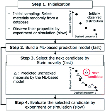
We show an overview of BLOX in Fig. 1. Our implementation of BLOX is available at http://github.com/tsudalab/BLOX. In BLOX, after the initial preparation step (Step 1), the search is performed by repeating the following three steps: the construction of a property prediction model (Step 2), the selection of a candidate using the Stein novelty score based on Stein discrepancy (Step 3), and the evaluation of the selected candidate by experiment or simulation (Step 4). The details of each step are as follows.In Step 1, a dataset of samples (materials/molecules) are chosen for searching and objective properties are determined. Two or more objective properties can be set. Here, there is no need to design an appropriate evaluation function and set a search region (boundary). A small amount of property data obtained from experiments or simulations is needed because BLOX uses ML to predict properties. Previously measured property data can be used, if available. If no property data is available, experiments or simulations must be conducted for a small number of randomly selected candidates. As a demonstration, in this study, we employed the ZINC database and selected 100![[thin space (1/6-em)]](https://www.rsc.org/images/entities/char_2009.gif) 000 commercially available molecules with small ZINC indexes from ZINC000000000007 to ZINC000002386999 as a candidate molecules database. We used the absorption wavelength for the first singlet excited (S1) state and its oscillator strength (as an alternative to the experimental intensity) as objective properties to find molecules. For the initial sampling, we selected 10 molecules randomly and calculated the values of their objective properties using DFT. The computational details are given in Step 4.
000 commercially available molecules with small ZINC indexes from ZINC000000000007 to ZINC000002386999 as a candidate molecules database. We used the absorption wavelength for the first singlet excited (S1) state and its oscillator strength (as an alternative to the experimental intensity) as objective properties to find molecules. For the initial sampling, we selected 10 molecules randomly and calculated the values of their objective properties using DFT. The computational details are given in Step 4.
In Step 2, an ML-based prediction model is built for the objective properties based on the already evaluated materials and their property data. Any method that can predict the desired properties of materials can be used. In our demonstration, as a simple example, we built two models for predicting the absorption wavelength and intensity using the Morgan fingerprint,26 which is widely used in chemoinformatics, and classical ML methods. For each molecule, we calculated its fingerprint, which is a 2048-dimensional vector consisting of values of 0 and 1, using RDKit.27 We normalized the calculated fingerprints and property values. For the training dataset (pairs of fingerprints and property values for already evaluated molecules), we train two prediction models using standard ML techniques, namely, Lasso regression,28 Ridge regression,29 support vector regression (SVR),30 random forest (RF),31 and neural network (NN). A first-degree polynomial function is employed as the basis function of Lasso and Ridge regression. Although it has been reported that NN-based methods such as Graph Convolutional Networks (GCNs)32 are superior in predicting chemical/physical properties of molecules,33–40 such NN-based methods, particularly deep NN-based models, generally require large dataset to be effective. In BLOX, it is required to train the prediction model with a very small dataset, especially at the beginning of the search. Therefore, in this study, we mainly used conventional ML methods. In this study, as the NN model, we utilized a multilayer perceptron used in the previous studies.33,34 The network has three hidden layers and the number of neurons in each layer is 500, 500, and 100. We used the scikit-learn library41 to perform the above calculations.
In Step 3, a candidate is selected for evaluation in Step 4 based on Stein discrepancy.23,24 First, for unchecked materials in the database, we predict their properties (open triangles in Step 3, Fig. 1) using the prediction models developed in Step 2. Most of the predicted points are expected to be distributed around some trends. However, the trends are generally undefined. Next, we select the most deviated candidate (triangle surrounded by the red circle in Step 3, Fig. 1) using Stein discrepancy (see the ESI† for computational details of Stein discrepancy). Fig. 2 illustrates the concept of Stein novelty (SN), which is our introduced index to select a next candidate, based on Stein discrepancy and the observed distribution. We can quantify the discrepancy SD(V) between the observed distribution V (Fig. 2a) and the uniform distribution U (Fig. 2b) using Stein discrepancy. Here, we evaluate the Stein discrepancies when a new point (predicted unchecked candidate) denoted by p is added to the observed distribution, as in Fig. 2c and d. If the new point deviates more from the observed distribution, as in Fig. 2c, its discrepancy is smaller. Then, we introduce SN to measure the degree of deviation, as given in the following equation:
| SN(V ∪ {p}) = SD(V) − SD(V ∪ {p}), | (1) |
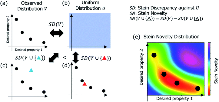 | ||
| Fig. 2 Stein discrepancy and novelty for the selection of the next candidate in Step 3 (Fig. 1). First, the discrepancy between the observed distribution V in (a) and the uniform distribution U in (b) is calculated using Stein discrepancy (SD(V)). When a new point (a mapped unchecked candidate) is added (blue triangle in (c) or red triangle in (d)), we can evaluate which distribution is more similar to the uniform distribution using Stein discrepancy. In this case, the distribution in (c) is more similar to the uniform distribution, that is, the deviation of the blue triangle from the observed distribution is greater than the deviation of the red triangle. The Stein novelty is the score used to measure this deviation (see the details in the main text), and the visualized Stein novelty for the observed distribution in (a) is shown in (e). | ||
In Step 4, the candidate selected in Step 3 is evaluated by experiment or simulation. In the demonstration, for the selected molecule, we calculate the absorption wavelength for the S1 state and its oscillator strength using DFT, as follows. A three-dimensional structure is converted from the molecule in SMILES string with RDKit. After optimizing its conformational structure at the universal force field (UFF) level, we optimize it using DFT at the B3LYP/6-31G* level. Then, we compute the absorption wavelength and the oscillator strength of the molecule using time-dependent DFT (TD-DFT) at the same level. For the TD-DFT computation, the lowest ten excited states are computed. All DFT calculations were performed with the Gaussian 16 package.42 In this study, when a calculation failed in the middle, we stopped the computation and instead performed the calculation for the molecule with the second-highest SN score.
Absorption spectra
We experimentally measured the absorption wavelengths and intensities of the selected test molecules (Table S1†). Test molecules were used as received expect for molecule (ii). Molecule (ii) was purified with column chromatography on silica gel since it involved some impurities in 1H-NMR analysis. Absorption spectra in solution were recorded using a Shimadzu UV-3600 UV-vis-NIR spectrophotometer. A quartz cell with 1 cm path length was used. Spectroscopic grade solvents, purchased from Tokyo Chemical Industry (TCI) and Wako Pure Chemical Industries, were used as received. Solvatochromic effect and concentration dependencies are detailed in the ESI.† To exclude the influence of trace impurities, test molecules were analysed by high performance liquid chromatography (HPLC) (see Table S3 and Fig. S23–S29†). It is confirmed that absorption spectra of main fractions in HPLC were consistent with the absorption spectra shown in Fig. 6. In addition, purity of test molecules were analyzed by HPLC. Note that molecule (i) was omitted in HPLC analysis due to the lack of measurable absorption spectrum. See ESI† for experimental details of HPLC.Characterization of test molecules
Test molecules were characterized by 1H-NMR spectrometry (Fig. S5–S12†) and high resolution mass spectrometry (HRMS, Table S2, Fig. S16–S22†). 1H-NMR spectra were obtained using an AL300 BX spectrometer (JEOL, 300 MHz). HRMS was recorded on a Bruker TIMS-TOF spectrometer with samples dissolved in 1![[thin space (1/6-em)]](https://www.rsc.org/images/entities/char_2009.gif) :
:![[thin space (1/6-em)]](https://www.rsc.org/images/entities/char_2009.gif) 1 acetonitrile
1 acetonitrile![[thin space (1/6-em)]](https://www.rsc.org/images/entities/char_2009.gif) :
:![[thin space (1/6-em)]](https://www.rsc.org/images/entities/char_2009.gif) methanol (0.1 mg mL−1).
methanol (0.1 mg mL−1).
Results and discussion
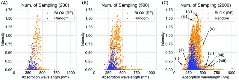
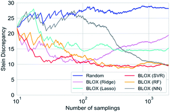
We performed a BLOX trial using RF-based prediction models to find out-of-trend molecules from the ZINC database using the absorption wavelength and intensity as objective properties. The orange points in Fig. 3 indicate the molecules (samples) found by BLOX sampling in the property space consisting of the absorption wavelength for the S1 state and its oscillator strength (intensity) after 200 (A), 500 (B), and 2000 (C) samplings. To compare the performance of BLOX with RF, we also sampled molecules randomly from the database and evaluated their properties (blue triangles, Fig. 3). The distribution obtained by random sampling suggests the presence of the trend, that is, molecules whose absorption wavelength distributed in the range of 250–400 nm with high intensities. In comparison, BLOX with RF (orange points, Fig. 3) successfully found out-of-trend molecules that have high intensities with shorter (<250 nm) and longer (>400 nm) absorption wavelengths. We picked molecules (i)–(viii) in Fig. 3C as examples of out-of-trend molecules for further experimental verification by UV-vis absorption spectrum measurements, as discussed later.To investigate the effect of different prediction models on the search results, we also performed BLOX trials using the Lasso, Ridge, SVR, and NN models. The initial 10 molecules were the same in all the searches, including the random sampling. Fig. S1† shows the search results using Lasso ((a)–(c)), Ridge ((d)–(f)), SVR ((g)–(i)), and NN ((j)–(l)). Fig. 3 and S1† clearly show that the molecules found using the RF and SVR models are distributed over a wide range, i.e., many out-of-trend molecules are found. To evaluate the difference between the prediction models quantitatively, we show the Stein discrepancy values as functions of the number of samplings in Fig. 4. A Stein discrepancy value closer to 0 indicates a greater similarity between the observed distribution and the uniform distribution, i.e., the obtained molecules are distributed more widely in the property space. The results in Fig. 4 show that the Stein discrepancy values decrease immediately after the start of sampling in all samplings using BLOX except for NN, and that the Stein discrepancy values of the BLOX trials are significantly lower than those of the random sampling. In addition, the nonlinear prediction models (SVR and RF) have lower Stein discrepancy values than the Lasso and Ridge models. From Fig. 4, NN finally showed high performance after 2000 sampling, but it was comparable to random search when the number of sampling is small. Thus, it was quantitatively confirmed that the molecules searched using RF and SVR were distributed over a wide range in the property space.
We adopted some ML methods to build the prediction models. As references, the performance of the predictions with RF and NN for the absorption wavelength and intensity are evaluated in Fig. S2 and S3 in ESI.† In RF, although the prediction accuracy in the demonstration was low when the number of evaluated data was small, this did not seem to cause fatal problems because the BLOX trials successfully found out-of-trend molecules more effectively than the random sampling, even with a small number of samplings, as shown in Fig. 4. Furthermore, the prediction accuracy of BLOX can be enhanced by increasing the amount of sample data. When the number of sampled molecules increases, the prediction accuracy is improved, as shown in Fig. S2C and F.† Recently, property prediction methods using various ML methods, including deep-learning techniques, have been proposed.32,37,38,43–50 As stated in the method section, although NN-based, particularly deep-learning-based, prediction models are known to have high accuracy, they are not always practical because the amount of data is limited and training time is required for each sampling in BLOX. In fact, from the prediction performances of the NN model as shown in Fig. S3,† we can see that the prediction accuracy is low when the number of training data is small, such as Fig. S3A, B, D and E,† whereas the accuracy improves with the increase of the number of training data, such as Fig. S3C and F.† Due to this low accuracy, out-of-trend molecules are not found at the beginning of search. Thus, it is important to use an appropriate ML technique so that the prediction accuracy is not too bad.
As another approach to increase the accuracy of the prediction model, Proppe et al. have proposed a strategy to select dissimilar molecules to use as a training dataset by combining Gaussian process and active learning to build an accurate prediction model of dispersion correction parameter in DFT calculations.51 Although their method has a different objective from BLOX, in the future, incorporating their method may improve the exploration performance of BLOX by enhancing the accuracy of the prediction model.
In addition, the framework of BLOX is applicable for other materials, if properties can be predicted to some extent using an ML-based model from materials descriptors. For example, in solid materials, the magpie descriptor has been reported for predicting physical properties such as superconducting temperature and bandgap.52,53 Also, in solid-state materials community, various types of descriptors for composition and structure of atoms have been prepared, and using some tools,54–56 we can easily obtain these descriptors using libraries like RDKit.27 For actual application of BLOX to other materials, it is required to select both an appropriate prediction model and a descriptor that match the dataset and target properties with taking a balance between the prediction accuracy and training time.
The time required for the BLOX search consists of three components: the time to train the ML-based prediction model (training time), the time to select the next candidates based on the SN (selection time), and the time to evaluate the selected candidate through experiments or simulations (evaluation time). The appropriate allocation of these computational times depends on the size of the database, the prediction model used, and the cost of the experiments or simulations. The training and selection times required in this study on a 12 core (Intel Xeon Gold 6148 CPU) server are shown in Fig. S4.† Although the calculation time tended to increase with an increase in the amount of observed data, the calculation was completed in a few tens of seconds to ∼2 min. The average simulation time on the same server was 29.74 min per molecule. Therefore, in this study, the training time for the ML-based prediction models and the selection time were sufficiently short in comparison with the evaluation time.
In this study, we used 100![[thin space (1/6-em)]](https://www.rsc.org/images/entities/char_2009.gif) 000 molecules in the ZINC dataset as an exploration demonstration. However, BLOX is applicable to a larger dataset because only the selection time increases when searching in a larger dataset. As shown in Fig. S4,† the selection time is much shorter than for experiments and detailed simulations, and these predictions and Stein novelty calculations for each material candidate in a dataset can be performed independently. This indicates that the selection time will only increase linearly with respect to the increase of the dataset size. In addition, because of the independence, the selection can be further accelerated by using more CPUs, while 12 CPUs were used in this study. Therefore, there is nothing to hinder our method from applying to a larger dataset. Furthermore, to explore an open chemical space beyond the finite dataset, the combination of BLOX and de novo molecule generation methods15,57–61 can be a promising approach. Most of these generation methods to generate molecules with target properties by sequentially evaluating the properties (scores) of the generated molecules. Here, using the BLOX framework (especially Step 2 and Step 3 in Fig. 1), we can evaluate the degree (scores) of deviation (out-of-trend) for generated de novo molecules. The BLOX framework would be extended to be truly boundless by combining such an evaluation strategy and de novo molecule generation.
000 molecules in the ZINC dataset as an exploration demonstration. However, BLOX is applicable to a larger dataset because only the selection time increases when searching in a larger dataset. As shown in Fig. S4,† the selection time is much shorter than for experiments and detailed simulations, and these predictions and Stein novelty calculations for each material candidate in a dataset can be performed independently. This indicates that the selection time will only increase linearly with respect to the increase of the dataset size. In addition, because of the independence, the selection can be further accelerated by using more CPUs, while 12 CPUs were used in this study. Therefore, there is nothing to hinder our method from applying to a larger dataset. Furthermore, to explore an open chemical space beyond the finite dataset, the combination of BLOX and de novo molecule generation methods15,57–61 can be a promising approach. Most of these generation methods to generate molecules with target properties by sequentially evaluating the properties (scores) of the generated molecules. Here, using the BLOX framework (especially Step 2 and Step 3 in Fig. 1), we can evaluate the degree (scores) of deviation (out-of-trend) for generated de novo molecules. The BLOX framework would be extended to be truly boundless by combining such an evaluation strategy and de novo molecule generation.
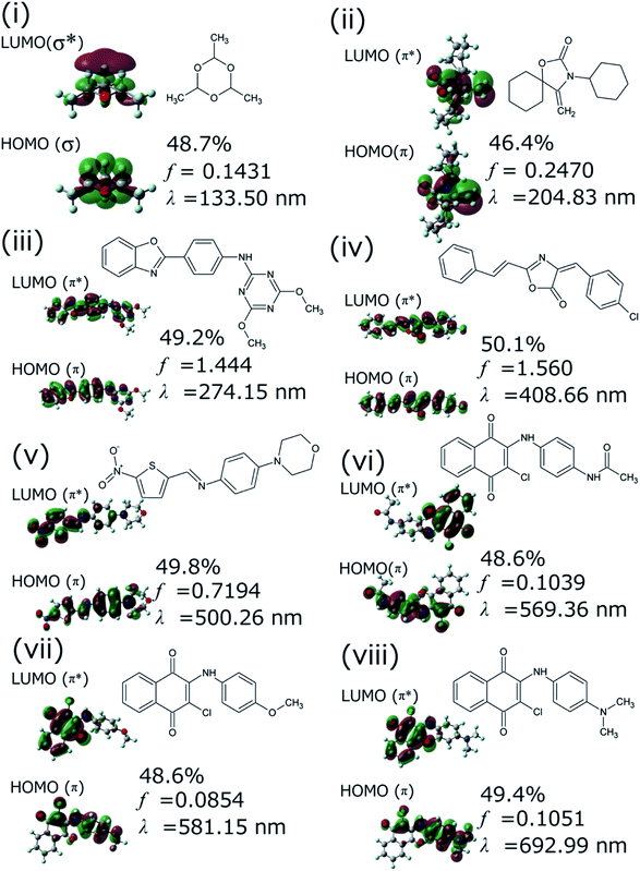
We successfully demonstrated the effectiveness of BLOX using the example of light absorption for molecules described at the DFT level. Hereafter, we discuss the validity from the experimental viewpoint considering the error of DFT. Each of the selected molecules ((i)–(viii) in Fig. 3C) is shown in Fig. 5 along with its dominant electronic transition to the S1 state calculated at the B3LYP/6-31G* level. The S1 state of each molecule is attributed to a HOMO–LUMO single electron transition. The excitation of (i) is attributed to σ–σ* excitation, as reflected by the high energy of the excitation (133.5 nm). For (ii)–(viii), the S1 excited states are attributed to π–π* excitation. In particular, the S1 states of (ii)–(iv) induce bond alternation (double bonds in the S0 state becomes single bonds in the S1 state). Hence, the oscillator strength is strong because the overlap between the HOMO and the LUMO is large. However, (v)–(viii) absorb light at wavelengths longer than 500 nm, indicating that the S1 states have charge-transfer properties. Thus, the overlap between the HOMO and the LUMO of each of these molecules is small, as reflected by their low oscillator strengths.
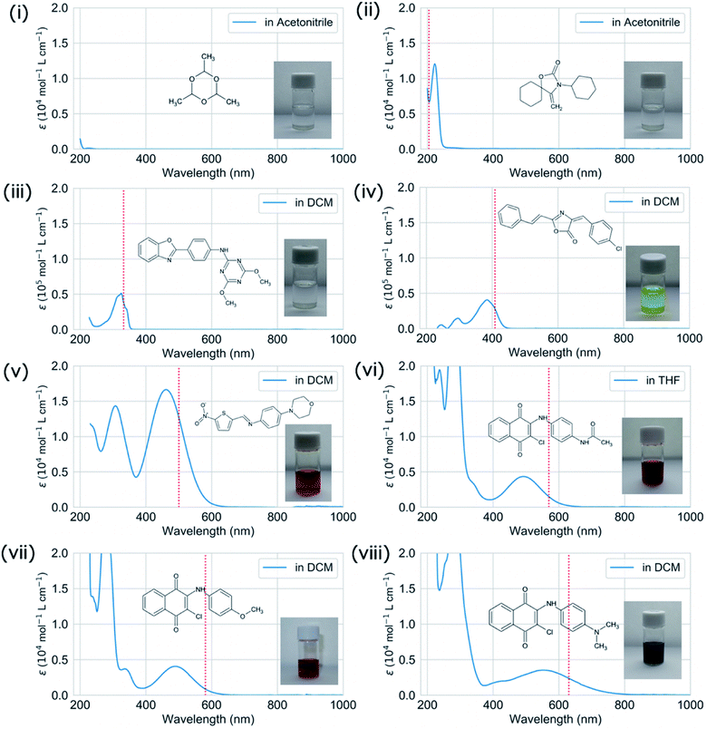
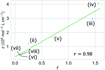
We validated the calculated absorption properties of (i)–(viii) using UV-vis absorption spectra measurements, as shown in Fig. 6 along with images of the solutions (see Fig. S13 and S14† for UV-vis absorption spectra at other concentrations and in other solvents, respectively). The solutions of (i)–(iii), which absorb light at wavelengths shorter than 300 nm, are transparent and colorless, whereas those of (iv)–(viii), which absorb light at wavelengths longer than 400 nm, are colored. We could not record the absorbance of molecule (i) in any available solvent. As mentioned previously, the S1 states of (v)–(viii) have charge-transfer properties, which results in a computational underestimation of the S1 energy,62 as reflected in Fig. 6(v)–(viii). However, the absorption spectra of (ii)–(viii) indicate that the experimental absorption peaks nearly correspond to the calculated S1 energies (broken red lines in Fig. 6). Concerning the intensity, the lowest energy absorption bands of (iii) and (iv) show high molar absorption coefficients on the order of 0.4 × 10⁵ mol−1 L cm−1, whereas those of the other molecules are at least 0.4 × 10⁴ mol−1 L cm−1. The molar absorption coefficients observed for (ii)–(viii) correlate well with the calculated oscillator strengths, as shown in Fig. 7. Therefore, the BLOX framework can find plausible molecules despite the evaluation being performed at the DFT level.
Herein, we employed the ZINC database, which consists of drug candidates. For example, (i) (paraldehyde) is widely used as a sedative, hypnotic, and anticonvulsant.63,64 (vii) has been reported as one of the anticancer drug candidates.65 However, as (iv)–(viii) are colored molecules, they may also be useful as benign dyes, e.g., for organic solar cells. Furthermore, (i) and (ii) may be useful as harmless UV filters that block strong light (at short wavelength). In a similar attempt, the repurposing of deoxyribonucleic acid topoisomerase inhibitors as organic semiconductors has also been reported.66 The results of our demonstration suggest that BLOX has the potential to accelerate the discovery of new materials by using databases collected for one purpose in other unintended fields.
Conclusion
In conclusion, we proposed a novel search method (BoundLess Objective-free eXploration; BLOX) for the effective discovery of out-of-trend materials from a dataset based on Stein discrepancy. Notably, BLOX does not require any information about the distribution of the materials in the property space as input. To demonstrate the utility of this method, we applied BLOX combined with DFT-based simulations to find light-absorbing molecules with high molar absorption coefficients in a database of drug candidates. BLOX showed better performances to find out-of-trend molecules, compared to random sampling. Furthermore, it was experimentally confirmed that the discovered compounds absorbed at the expected wavelengths. We believe that this method will be useful for finding unexpected and out-of-trend materials that have the potential to push their property limits by developing derivatives.Conflicts of interest
There are no conflicts to declare.Acknowledgements
This work is supported by a project subsidized by the New Energy and Industrial Technology Development Organization (NEDO) and the Ministry of Education, Culture, Sports, Science, and Technology of Japan (MEXT) as a “Priority Issue on Post-K Computer” (Building Innovative Drug Discovery Infrastructure through Functional Control of Biomolecular Systems). K. Tsuda is supported by NEDO P15009, SIP (Technologies for Smart Bio-industry and Agriculture), JST CREST JPMJCR1502, and JST ERATO JPMJER1903. This research used the computational resources of the supercomputer centers of NIMS and RAIDEN of AIP (RIKEN).Notes and references
- R. Ramakrishnan, M. Hartmann, E. Tapavicza and O. A. von Lilienfeld, J. Chem. Phys., 2015, 143, 084111 CrossRef PubMed.
- H. Kaji, H. Suzuki, T. Fukushima, K. Shizu, K. Suzuki, S. Kubo, T. Komino, H. Oiwa, F. Suzuki, A. Wakamiya, Y. Murata and C. Adachi, Nat. Commun., 2015, 6, 8476 CrossRef CAS PubMed.
- P. Brogdon, H. Cheema and J. H. Delcamp, ChemSusChem, 2018, 11, 86–103 CrossRef CAS PubMed.
- N. A. Shaath, Photochem. Photobiol. Sci., 2010, 9, 464–469 RSC.
- R. Gómez-Bombarelli, J. Aguilera-Iparraguirre, T. D. Hirzel, D. Duvenaud, D. Maclaurin, M. A. Blood-Forsythe, H. S. Chae, M. Einzinger, D.-G. Ha, T. Wu, G. Markopoulos, S. Jeon, H. Kang, H. Miyazaki, M. Numata, S. Kim, W. Huang, S. I. Hong, M. Baldo, R. P. Adams and A. Aspuru-Guzik, Nat. Mater., 2016, 15, 1120–1127 CrossRef.
- R. G. Parr, in Horizons of Quantum Chemistry, ed. K. Fukui and B. Pullman, Springer, Dordrecht, 1980, pp. 5–15 Search PubMed.
- B. Shahriari, K. Swersky, Z. Wang, R. P. Adams and N. de Freitas, Proc. IEEE, 2016, 104, 148–175 Search PubMed.
- A. Seko, A. Togo, H. Hayashi, K. Tsuda, L. Chaput and I. Tanaka, Phys. Rev. Lett., 2015, 115, 205901 CrossRef.
- S. Ju, T. Shiga, L. Feng, Z. Hou, K. Tsuda and J. Shiomi, Phys. Rev. X, 2017, 7, 021024 Search PubMed.
- Y. Saito, M. Oikawa, H. Nakazawa, T. Niide, T. Kameda, K. Tsuda and M. Umetsu, ACS Synth. Biol., 2018, 7, 2014–2022 CrossRef CAS PubMed.
- A. M. Gopakumar, P. V. Balachandran, D. Xue, J. E. Gubernatis and T. Lookman, Sci. Rep., 2018, 8, 3738 CrossRef PubMed.
- A. Sakurai, K. Yada, T. Simomura, S. Ju, M. Kashiwagi, H. Okada, T. Nagao, K. Tsuda and J. Shiomi, ACS Cent. Sci., 2019, 5, 319–326 CrossRef CAS PubMed.
- K. Terayama, K. Tsuda and R. Tamura, Jpn. J. Appl. Phys., 2019, 58, 098001 CrossRef CAS.
- J. M. Hernández-Lobato, J. Requeima, E. O. Pyzer-Knapp and A. Aspuru-Guzik, in Proceedings of the 34th International Conference on Machine Learning, Sydney, 2017, pp. 1470–1479 Search PubMed.
- R. Gómez-Bombarelli, J. N. Wei, D. Duvenaud, J. M. Hernández-Lobato, B. Sánchez-Lengeling, D. Sheberla, J. Aguilera-Iparraguirre, T. D. Hirzel, R. P. Adams and A. Aspuru-Guzik, ACS Cent. Sci., 2018, 4, 268–276 CrossRef PubMed.
- R.-R. Griffiths and J. M. Hernández-Lobato, Chem. Sci., 2020, 11, 577–586 RSC.
- R. Winter, F. Montanari, A. Steffen, H. Briem, F. Noé and D.-A. Clevert, Chem. Sci., 2019, 10, 8016–8024 RSC.
- K. Deb, in Search Methodologies: Introductory Tutorials in Optimization and Decision Support Technique, Springer, New York, 2014, pp. 403–449 Search PubMed.
- M. T. Emmerich, A. H. Deutz and J. W. Klinkenberg, in 2011 IEEE Congress of Evolutionary Computation (CEC), IEEE, New Orleans, 2011, pp. 2147–2154 Search PubMed.
- J. Lehman and K. O. Stanley, Evol. Comput., 2011, 19, 189–223 CrossRef PubMed.
- A. Baranes and P.-Y. Oudeyer, Robot. Autonom. Syst., 2013, 61, 49–73 CrossRef.
- J. Grizou, L. J. Points, A. Sharma and L. Cronin, Sci. Adv., 2020, 6, eaay4237 CrossRef PubMed.
- C. Stein, Approximate Computation of Expectations, Institute of Mathematical Statistics, Hayward, CA, 1986 Search PubMed.
- Q. Liu, J. Lee and M. Jordan, in Proceedings of the 33rd International Conference on Machine Learning, New York, 2016, pp. 276–284 Search PubMed.
- J. J. Irwin, T. Sterling, M. M. Mysinger, E. S. Bolstad and R. G. Coleman, J. Chem. Inf. Model., 2012, 52, 1757–1768 CrossRef CAS PubMed.
- D. Rogers and M. Hahn, J. Chem. Inf. Model., 2010, 50, 742–754 CrossRef CAS PubMed.
- RDKit: Open-Source Cheminformatics Software, 2019 Search PubMed.
- R. Tibshirani, J. Roy. Stat. Soc. B, 1996, 58, 267–288 Search PubMed.
- A. E. Hoerl and R. W. Kennard, Technometrics, 1970, 12, 55–67 CrossRef.
- A. J. Smola and B. Schölkopf, Stat. Comput., 2004, 14, 199–222 CrossRef.
- L. Breiman, Mach. Learn., 2001, 45, 5–32 CrossRef.
- D. K. Duvenaud, D. Maclaurin, J. Iparraguirre, R. Bombarell, T. Hirzel, A. Aspuru-Guzik and R. P. Adams, in Advances in Neural Information Processing Systems 28, ed. C. Cortes, N. D. Lawrence, D. D. Lee, M. Sugiyama and R. Garnett, Curran Associates, Inc., 2015, pp. 2224–2232 Search PubMed.
- K.-Z. Myint, L. Wang, Q. Tong and X.-Q. Xie, Mol. Pharm., 2012, 9, 2912–2923 CrossRef CAS PubMed.
- E. O. Pyzer-Knapp, K. Li and A. Aspuru-Guzik, Adv. Funct. Mater., 2015, 25, 6495–6502 CrossRef CAS.
- J. N. Wei, D. Duvenaud and A. Aspuru-Guzik, ACS Cent. Sci., 2016, 2, 725–732 CrossRef CAS PubMed.
- J. Jiménez, M. Škalič, G. Martínez-Rosell and G. De Fabritiis, J. Chem. Inf. Model., 2018, 58, 287–296 CrossRef.
- F. Häse, C. Kreisbeck and A. Aspuru-Guzik, Chem. Sci., 2017, 8, 8419–8426 RSC.
- Z. Wu, B. Ramsundar, E. N. Feinberg, J. Gomes, C. Geniesse, A. S. Pappu, K. Leswing and V. Pande, Chem. Sci., 2018, 9, 513–530 RSC.
- S. Ishida, K. Terayama, R. Kojima, K. Takasu and Y. Okuno, J. Chem. Inf. Model., 2019, 59, 5026–5033 CrossRef CAS PubMed.
- K. Ghosh, A. Stuke, M. Todorović, P. B. Jørgensen, M. N. Schmidt, A. Vehtari and P. Rinke, Adv. Sci., 2019, 6, 1801367 CrossRef PubMed.
- F. Pedregosa, G. Varoquaux, A. Gramfort, V. Michel, B. Thirion, O. Grisel, M. Blondel, P. Prettenhofer, R. Weiss, V. Dubourg, J. Vanderplas, A. Passos, D. Cournapeau, M. Brucher, M. Perrot and É. Duchesnay, J. Mach. Learn. Res., 2011, 12, 2825–2830 Search PubMed.
- M. J. Frisch, G. W. Trucks, H. B. Schlegel, G. E. Scuseria, M. A. Robb, J. R. Cheeseman, G. Scalmani, V. Barone, G. A. Petersson, H. Nakatsuji, X. Li, M. Caricato, A. V. Marenich, J. Bloino, B. G. Janesko, R. Gomperts, B. Mennucci, H. P. Hratchian, J. V. Ortiz, A. F. Izmaylov, J. L. Sonnenberg, D. Williams-Young, F. Ding, F. Lipparini, F. Egidi, J. Goings, B. Peng, A. Petrone, T. Henderson, D. Ranasinghe, V. G. Zakrzewski, J. Gao, N. Rega, G. Zheng, W. Liang, M. Hada, M. Ehara, K. Toyota, R. Fukuda, J. Hasegawa, M. Ishida, T. Nakajima, Y. Honda, O. Kitao, H. Nakai, T. Vreven, K. Throssell, J. A. Montgomery Jr, J. E. Peralta, F. Ogliaro, M. J. Bearpark, J. J. Heyd, E. N. Brothers, K. N. Kudin, V. N. Staroverov, T. A. Keith, R. Kobayashi, J. Normand, K. Raghavachari, A. P. Rendell, J. C. Burant, S. S. Iyengar, J. Tomasi, M. Cossi, J. M. Millam, M. Klene, C. Adamo, R. Cammi, J. W. Ochterski, R. L. Martin, K. Morokuma, O. Farkas, J. B. Foresman and D. J. Fox, Gaussian 16 (Revision A), Gaussian, Inc., Wallingford, CT, 2016 Search PubMed.
- A. P. Bartók, S. De, C. Poelking, N. Bernstein, J. R. Kermode, G. Csányi and M. Ceriotti, Sci. Adv., 2017, 3, e1701816 CrossRef PubMed.
- G. Montavon, M. Rupp, V. Gobre, A. Vazquez-Mayagoitia, K. Hansen, A. Tkatchenko, K.-R. Müller and O. Anatole von Lilienfeld, New J. Phys., 2013, 15, 095003 CrossRef.
- K. T. Butler, D. W. Davies, H. Cartwright, O. Isayev and A. Walsh, Nature, 2018, 559, 547–555 CrossRef CAS PubMed.
- M. Rupp, A. Tkatchenko, K.-R. Müller and O. A. von Lilienfeld, Phys. Rev. Lett., 2012, 108, 058301 CrossRef PubMed.
- J. Behler, J. Chem. Phys., 2016, 145, 170901 CrossRef PubMed.
- F. A. Faber, L. Hutchison, B. Huang, J. Gilmer, S. S. Schoenholz, G. E. Dahl, O. Vinyals, S. Kearnes, P. F. Riley and O. A. von Lilienfeld, J. Chem. Theory Comput., 2017, 13, 5255–5264 CrossRef CAS PubMed.
- E. N. Feinberg, D. Sur, Z. Wu, B. E. Husic, H. Mai, Y. Li, S. Sun, J. Yang, B. Ramsundar and V. S. Pande, ACS Cent. Sci., 2018, 4, 1520–1530 CrossRef CAS PubMed.
- C. Nyshadham, M. Rupp, B. Bekker, A. V. Shapeev, T. Mueller, C. W. Rosenbrock, G. Csányi, D. W. Wingate and G. L. W. Hart, npj Comput. Mater., 2019, 5, 51 CrossRef.
- J. Proppe, S. Gugler and M. Reiher, J. Chem. Theory Comput., 2019, 15, 6046–6060 CrossRef CAS PubMed.
- L. Ward, A. Agrawal, A. Choudhary and C. Wolverton, npj Comput. Mater., 2016, 2, 16028 CrossRef.
- V. Stanev, C. Oses, A. G. Kusne, E. Rodriguez, J. Paglione, S. Curtarolo and I. Takeuchi, npj Comput. Mater., 2018, 4, 29 CrossRef.
- L. Ward, A. Dunn, A. Faghaninia, N. E. R. Zimmermann, S. Bajaj, Q. Wang, J. Montoya, J. Chen, K. Bystrom, M. Dylla, K. Chard, M. Asta, K. A. Persson, G. J. Snyder, I. Foster and A. Jain, Comput. Mater. Sci., 2018, 152, 60–69 CrossRef.
- L. Himanen, M. O. J. Jäger, E. V. Morooka, F. Federici Canova, Y. S. Ranawat, D. Z. Gao, P. Rinke and A. S. Foster, Comput. Phys. Commun., 2020, 247, 106949 CrossRef CAS.
- H. Yamada, C. Liu, S. Wu, Y. Koyama, S. Ju, J. Shiomi, J. Morikawa and R. Yoshida, ACS Cent. Sci., 2019, 5, 1717–1730 CrossRef CAS PubMed.
- X. Yang, J. Zhang, K. Yoshizoe, K. Terayama and K. Tsuda, Sci. Technol. Adv. Mater., 2017, 18, 972–976 CrossRef CAS PubMed.
- M. H. S. Segler, T. Kogej, C. Tyrchan and M. P. Waller, ACS Cent. Sci., 2018, 4, 120–131 CrossRef CAS PubMed.
- B. Sanchez-Lengeling and A. Aspuru-Guzik, Science, 2018, 361, 360 CrossRef CAS PubMed.
- N. Yoshikawa, K. Terayama, M. Sumita, T. Homma, K. Oono and K. Tsuda, Chem. Lett., 2018, 47, 1431–1434 CrossRef CAS.
- J. H. Jensen, Chem. Sci., 2019, 10, 3567–3572 RSC.
- A. Dreuw and M. Head-Gordon, J. Am. Chem. Soc., 2004, 126, 4007–4016 CrossRef CAS PubMed.
- F. López-Muñoz, R. Ucha-Udabe and C. Alamo, Neuropsychiatr. Dis. Treat., 2005, 1, 329–343 Search PubMed.
- A. G. Rowland, A. M. Gill, A. B. Stewart, R. E. Appleton, A. Al Kharusi, C. Cramp and L.-K. Yeung, Arch. Dis. Child., 2009, 94, 720–723 CrossRef CAS PubMed.
- J. Benites, J. A. Valderrama, K. Bettega, R. C. Pedrosa, P. B. Calderon and J. Verrax, Eur. J. Med. Chem., 2010, 45, 6052–6057 CrossRef CAS PubMed.
- F. Zhang, V. Lemaur, W. Choi, P. Kafle, S. Seki, J. Cornil, D. Beljonne and Y. Diao, Nat. Commun., 2019, 10, 4217 CrossRef PubMed.
Footnote |
| † Electronic supplementary information (ESI) available: The details of BLOX and experimental spectroscopic data. See DOI: 10.1039/d0sc00982b |
| This journal is © The Royal Society of Chemistry 2020 |

