 Open Access Article
Machine learning dihydrogen activation in the chemical space surrounding Vaska's complex†‡
Pascal
Friederich
 abc,
Gabriel
dos Passos Gomes
 ac,
Riccardo
De Bin
d,
Alán
Aspuru-Guzik
*acef and
David
Balcells
 *g
*g
aChemical Physics Theory Group, Department of Chemistry, University of Toronto, Toronto, Ontario M5S 3H6, Canada
bInstitute of Nanotechnology, Karlsruhe Institute of Technology, Hermann-von-Helmholtz-Platz 1, 76344 Eggenstein-Leopoldshafen, Germany
cDepartment of Computer Science, University of Toronto, 214 College St., Toronto, Ontario M5T 3A1, Canada
dDepartment of Mathematics, University of Oslo, P. O. Box 1053, Blindern, N-0316, Oslo, Norway
eVector Institute for Artificial Intelligence, 661 University Ave. Suite 710, Toronto, Ontario M5G 1M1, Canada
fLebovic Fellow, Canadian Institute for Advanced Research (CIFAR), 661 University Ave, Toronto, ON M5G 1M1, Canada
gHylleraas Centre for Quantum Molecular Sciences, Department of Chemistry, University of Oslo, P. O. Box 1033, Blindern, N-0315, Oslo, Norway. E-mail: david.balcells@kjemi.uio.no
First published on 7th April 2020
Abstract
Homogeneous catalysis using transition metal complexes is ubiquitously used for organic synthesis, as well as technologically relevant in applications such as water splitting and CO2 reduction. The key steps underlying homogeneous catalysis require a specific combination of electronic and steric effects from the ligands bound to the metal center. Finding the optimal combination of ligands is a challenging task due to the exceedingly large number of possibilities and the non-trivial ligand–ligand interactions. The classic example of Vaska's complex, trans-[Ir(PPh3)2(CO)(Cl)], illustrates this scenario. The ligands of this species activate iridium for the oxidative addition of hydrogen, yielding the dihydride cis-[Ir(H)2(PPh3)2(CO)(Cl)] complex. Despite the simplicity of this system, thousands of derivatives can be formulated for the activation of H2, with a limited number of ligands belonging to the same general categories found in the original complex. In this work, we show how DFT and machine learning (ML) methods can be combined to enable the prediction of reactivity within large chemical spaces containing thousands of complexes. In a space of 2574 species derived from Vaska's complex, data from DFT calculations are used to train and test ML models that predict the H2-activation barrier. In contrast to experiments and calculations requiring several days to be completed, the ML models were trained and used on a laptop on a time-scale of minutes. As a first approach, we combined Bayesian-optimized artificial neural networks (ANN) with features derived from autocorrelation and deltametric functions. The resulting ANNs achieved high accuracies, with mean absolute errors (MAE) between 1 and 2 kcal mol−1, depending on the size of the training set. By using a Gaussian process (GP) model trained with a set of selected features, including fingerprints, accuracy was further enhanced. Remarkably, this GP model minimized the MAE below 1 kcal mol−1, by using only 20% or less of the data available for training. The gradient boosting (GB) method was also used to assess the relevance of the features, which was used for both feature selection and model interpretation purposes. Features accounting for chemical composition, atom size and electronegativity were found to be the most determinant in the predictions. Further, the ligand fragments with the strongest influence on the H2-activation barrier were identified.
Introduction
The reactivity of transition metal complexes plays a fundamental role in homogeneous catalysis. Crucially important reactions, such as water splitting1–7 and CO2 reduction,8–12 require metal catalysts in which ligands are combined to provide the optimal balance between activity, robustness, and selectivity. Computational chemistry has become a powerful tool in homogeneous catalysis, and combined with experiments, delivers molecular models enabling the rational design of catalytic systems.13–22 However, the key ligands and substituents of these models are classified with generic labels (e.g., ‘strong π-acceptor’, ‘bulky’ or ‘proton-acceptor’) that can be assigned to tens or hundreds of known compounds. The combination of all these possibilities yields a region of the chemical space23 containing thousands of catalyst candidates. Within these spaces, the presence of a small number of optimal catalysts is highly probable, but their discovery is a non-trivial task.24,25The systematic experimental characterization of thousands of homogeneous catalysts is impractical. High-throughput screening (HTS) techniques enable hundreds of tests combining multiple substrates and reaction conditions in a short time-scale.26–29 However, these techniques are typically limited to the testing of only tens of different catalysts. The scope of the HTS approach can be expanded with predictive quantitative structure–activity relationship (QSAR),30–34 and multivariate linear regression (MLR) models35–39 in which the empirical data are correlated to molecular descriptors.
An alternative to experimental HTS is the use of virtual screening (VS) methods, in which both the descriptors and the target property (e.g., catalytic activity or selectivity) are computed.40–44 The application of VS to transition metal catalysis is encumbered by the need for accurate results on thousands of systems. The proper description of chemical reactivity requires the use of quantum chemistry (QC) methods such as density functional theory (DFT), which has a computational cost that quickly becomes prohibitive. Further, transition states are challenging to converge.
From a computational perspective, machine learning (ML) is an attractive tool to complement QC methods. With appropriate training (i.e., optimization of the model parameters by error minimization), ML methods can make reliable X → y predictions from large and complex data (X = features, i.e., descriptors; y = target, i.e., a property of interest). While training of the models can be done with several hundreds of data points, the ML models allow evaluating the properties of thousands of additional data points rapidly. Such a feature enables the efficient search of new systems with optimal y values, which can be later synthesized and tested in the lab. Further features, including generative models and inverse design are also possible.45–50 Computational affordability is a key advantage of ML – a laptop can be used to train a model and make predictions in a timescale of minutes.
In contrast, running the advanced methods and models of modern QC requires several days in a supercomputer. ML approaches have already proven successful in different fields of chemistry,51–53 with a strong focus on materials science54–61 and drug discovery.62–68 In other areas, including organic synthesis,69–73 and theoretical74–81 and inorganic82,83 chemistry, the use of ML is rapidly growing. In catalysis,84,85 several examples have been reported for both heterogeneous86–93 and homogeneous94–98 systems.
The application of ML methods is strongly dependent on the accuracy, affordability, and explainability of the final model. High accuracy can be achieved when large data sets are available for training. Unfortunately, in the field of homogeneous catalysis, large data sets are neither available nor affordable. The catalysis of a particular reaction is typically proven for only a few tens (or less) of metal complexes. The possibility of learning from synthetic data generated in silico99–101 is appealing, but in practice accurate QC calculations are expensive. In this context, optimizing the ratio between accuracy and the size of the training data is imperative. Another challenge with many ML methods is the potential lack of interpretability; e.g., artificial neural networks (ANNs)102–109 may achieve high accuracy, but their predictions are difficult to interpret and explain with the language used in chemistry textbooks.
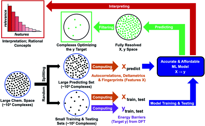
In this work, we assess the reliability of a computational protocol combining QC with ML for predicting the reactivity of transition metal complexes (Fig. 1). The protocol starts by defining a large region of the chemical space containing thousands of complexes, which are all described with computationally affordable descriptors110–112 (features X). In the next step, the chemical space is randomly split into two sets – a small set for training and testing, plus a large predicting set. The reaction energy barrier of interest (target y) is computed with an expensive DFT method for the training and testing sets. The {X, y} data of these sets are then used to optimize an accurate ML model. At the final stage of the protocol, the model is fed with the features describing the predicting set, delivering the energy barrier for all complexes. The optimal complexes are extracted by applying a simple filter (e.g., species minimizing the energy barrier). In the final step, the predictions are interpreted by ranking the relevance of the features.
The feasibility and reliability of the computational protocol shown in Fig. 1 were assessed for the activation of H2 within a substantial chemical space region derived from Vaska's complex, [Ir(PPh3)2(CO)(Cl)],113,114 which was used as a case study. H2-activation by transition metals plays a major role in hydrogenation processes used in the production of drugs and materials.115–118 The performances of different ML models were compared, showing that their combination with DFT calculations allows for the accurate, affordable, and explainable prediction of the reactivity of the complexes in the activation of H2. In this proof-of-concept application, both the energy barrier and the features were computed for the entire region of the chemical space studied. In future applications, the QC calculations will be carried out only for small training and testing sets, making the overall protocol affordable for large chemical spaces related to different reactions.
Results and discussion
Definition of the chemical space region of study
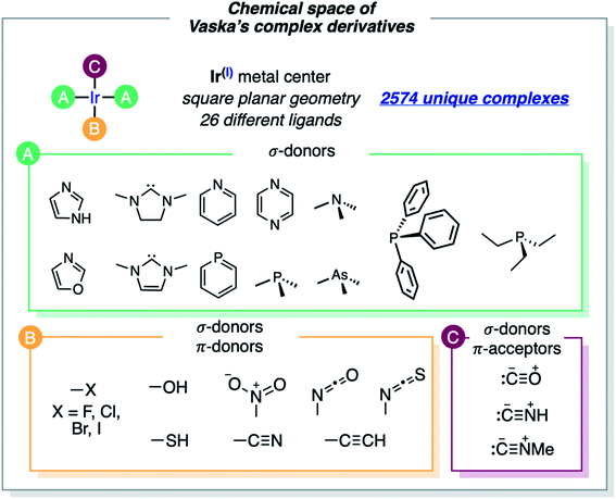
The formula of Vaska's [Ir(PPh3)2(CO)(Cl)] complex was generalized to [Ir(σd)2(σd,πa)(σ,πd)] by considering the σ/π electron-donor (d) and -acceptor (a) character of the ligands (Fig. 2). The three different ligand sets A, B and C were populated with 12 (neutral σd), 11 (anionic σ,πd) and 3 (neutral σd,πa) ligands, respectively, which overall yielded 2574 unique complexes, when combined in the trans Ir(I) square planar framework of the system (the A positions in trans were filled by either the same or two different ligands). In addition to the triphenylphosphine ligand of Vaska's complex, the σd ligand set included imidazole, oxazole, IMe (i.e. 1,3-dimethyl-imidazol-2-ylidene), SIMe (i.e. saturated IMe), pyridine, phosphinine, trimethylamine, pyrazine, trimethylphosphine, trimethylarsine, and triethylphosphine. The σd,πa ligand set included carbonyl as well as hydrogen- and methyl-isocyanide, whereas the σ,πd ligand set included hydroxy, thiolate, cyanide, nitrite, acetylide, isocyanate, isothiocyanate and all halogens (F, Cl, Br and I).Some of the ligands labeled above as π-acceptors can also have a soft π-donor character, and the opposite. Larger ligands and alternative binding models (e.g., O- and S-coordination of the isocyanate and isothiocyanate ligands) were not considered. The cis-coordination of the A ligands, which would be accessible with the smallest, was not considered either. The omission of these structural variations saves computation time, though it also limits the applicability of the resulting models.
Computational exploration of activation energies
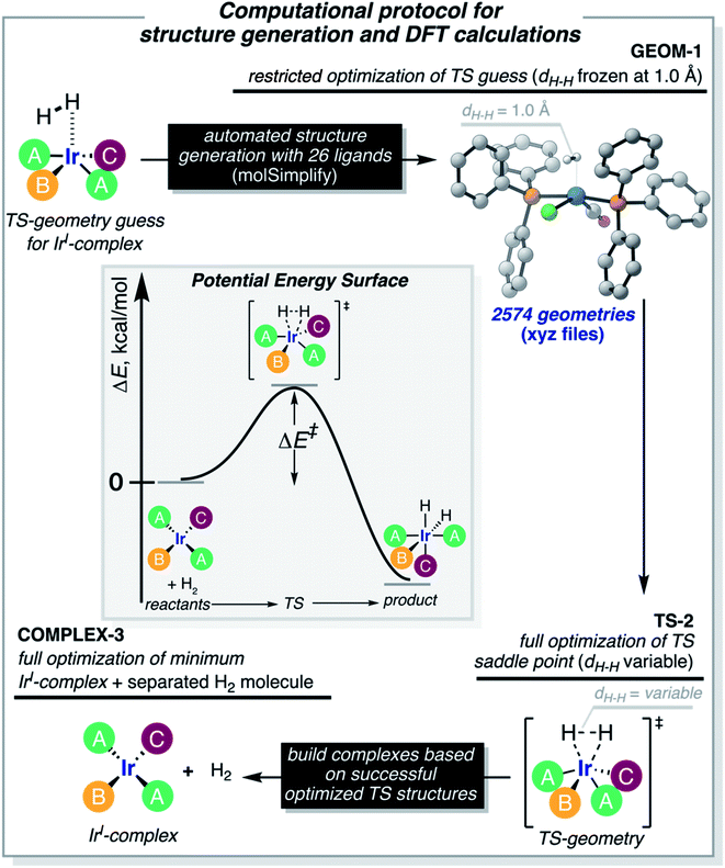
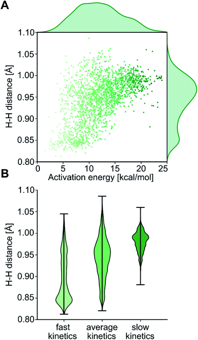
The computational protocol used in this work is illustrated in Fig. 3. The 2574 geometry guesses required to optimize the transition states were generated using the molSimplify library developed by Kulik and coworkers.119 All geometries were based on an iridium penta-coordinated core in a trigonal bipyramid geometry. Four coordination sites, including the two axial positions, were filled as shown in Fig. 2, with the ligands pre-optimized at the DFT level. The remaining equatorial position was capped with a dihydrogen ligand-activated with an elongated H–H distance (dHH) of 1.00 Å. For each system, three different DFT calculations were executed sequentially; namely: GEOM-1: restricted optimization to energy minimum by relaxing all geometrical parameters except dHH (frozen at 1.00 Å); TS-2: transition state optimization by computing the force constants at the first point and relaxing all geometrical parameters, including dHH; and COMPLEX-3: full optimization to energy minimum by relaxing all geometrical parameters, after removing the H2 fragment. GEOM-1 yielded the starting geometry used in the TS-2 calculation, facilitating the convergence of the latter. TS-2 yielded the transition state for H2-activation. COMPLEX-3 yielded the iridium complex reactant. The energy barrier for H2-activation (ΔE‡HH) was computed from the potential energies converged in TS-2 and COMPLEX-3, and that of H2 computed at the same level of theory. The H–H distance optimized at the transition state (d‡HH) was extracted from TS-2.After cleaning the data (see Fig. S1‡†), Fig. 4A shows the activation barriers ΔE‡HH and H–H distances d‡HH in the transition state for all 1947 converged complexes obtained in the high-throughput virtual screening approach described above. The {d‡HH, ΔE‡HH} data had minimum and maximum values of 0.81 Å/1.6 kcal mol−1 and 1.09 Å/25.6 kcal mol−1, respectively. The mean and standard deviation values were (0.94 ± 0.05) Å and (12.0 ± 4.3) kcal mol−1, respectively. The distribution of d‡HH shows a sharp peak at 0.96 Å, whereas the distribution of ΔE‡HH is flatter with a plateau between 7 and 15 kcal mol−1 (see Fig. S2‡†). Overall, the computed ΔE‡HH spans a wide range of energy values of ca. 20 kcal mol−1. The violin plot in Fig. 4B shows the correlation between d‡HH and ΔE‡HH, with fast activation (arbitrarily defined as 1.5 ≤ ΔE‡HH ≤ 8.1 kcal mol−1) mostly associated with smaller d‡HH values, and slow activation (arbitrarily defined as 15.1 ≤ ΔE‡HH ≤ 25.6 kcal mol−1) mostly associated with larger d‡HH values, as expected.
Data analysis and interpretation with machine learning methods
The high throughput virtual screening study presented in this work aims at a complete computational exploration of the defined chemical space of Vaska's complexes. However, the data generated in this approach can also be used to explore the possibility of using machine learning-based methods for the acceleration of future screening efforts. If machine learning models can reliably learn from a sparse subset of the chemical design space, these models can be used to efficiently estimate the properties of the remaining catalysts and thus be used to accelerate the exploration of more complex reactions and catalysts. In the following sections, we explore ways to train such machine learning models and compare hand-crafted and generic techniques to generate input representations for machine learning models.Features used in the description of Vaska's complex region of the chemical space
The features used to represent the complexes were computed with the full autocorrelation (FA) functions (eqn (1)). | (1) |
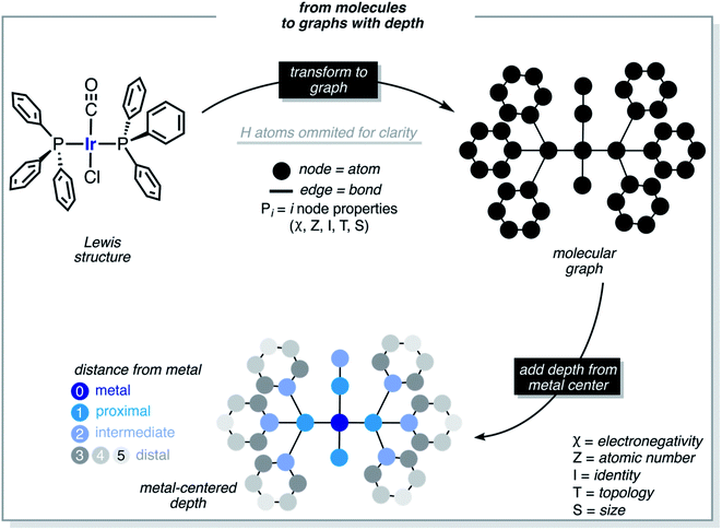
These functions provide a fingerprint of each complex by adding atomic property products (PiPj) computed for all atoms. i and j are the atomic indexes of the molecular graph representing the complex (Fig. 5). The atomic properties (P) include electronegativity (χ), atomic number (Z), identity (I; i.e., 1 for each position in the molecular graph), topology (T; i.e., coordination number) and size (S; i.e., covalent radius). Each property product is multiplied by the Dirac delta δ(di,j, d) function, in which di,j is the shortest distance between positions i and j in chemical bonds. The parameter d (depth) is the maximum distance in chemical bonds considered in the calculation of Pd. The autocorrelation function encodes the composition (Z), and the electronic (χ, T) and steric (I, S) properties of the complexes.
Each metal complex is represented by a single size-independent vector of features of dimensionality 5(d + 1). E.g., with d = 3, each metal complex is represented by the 20D vector shown in eqn (2).
| complexk = (χ0, χ1, χ2, χ3, Z0, Z1, Z2, Z3, I0, I1, I2, I3, T0, T1, T2, T3, S0, S1, S2, S3)k | (2) |
In addition to FA, other feature sets were tested, including the MA (metal-centered autocorrelations), MD (metal-centered deltametrics), and MAD (mixed metal-centered autocorrelations and deltametrics). MA features were computed with eqn (1) by setting the metal center as the depth origin (i.e. d = 0 at iridium) defining the proximal (d = 1), intermediate (d = 2) and distal (d > 2) regions (Fig. 5). MD features were computed with the deltametric functions shown in eqn (3), in which, relative to eqn (1), property products are replaced by property differences. MAD features were computed by applying eqn (1) to all features except electronegativity, for which eqn (3) was used to encode bond polarization (i.e., χi − χj), owing to the relevance of this property in chemical reactivity.
 | (3) |
We note that all metal-centered autocorrelations functions have the same factor PIr which does not play a role in the training of our machine learning models, as all input features are normalized before feeding them into the model. The choice of autocorrelations and deltametrics was motivated by their low computational cost and the work of Kulik.82,83 More conventional ligand descriptors24 were not considered but may also yield high accuracy.
Scatter plots were used for a visual exploration of the possible correlations between these features and the H2-activation barriers (Fig. S3‡†). The χ1 feature of the MD set, which quantifies the polarization of the Ir–ligand bonds, correlates with ΔE‡HH. The barrier becomes lower with the decreasing polarization of the Ir–ligand bonds, in which Ir is always the least electronegative element; i.e., electron-rich metal centers promote H2-activation by oxidative addition, as expected. The S2 feature of the MA set, which is related to the number of atoms and size of the second coordination shell (i.e., intermediate layer in Fig. 5), also correlates with ΔE‡HH. In this case, the barrier becomes lower with the increasing value of S2. The comparative analysis between different scatter plots also provided chemical insight. E.g. the combined analysis of the I-2 and S-2 plots (Fig. S4‡†) revealed the following two trends: (1) when the electron-withdrawing character of the nitrite ligand is compensated by two ER3 ligands (E = N, P, As), low barriers (i.e., ΔE‡HH < 10 kcal mol−1) are obtained, whereas, in contrast, (2) the H2-activation barriers involving the OH and SH ligands are, on average, higher than those computed in the absence of these ligands.
Artificial neural networks trained on autocorrelation features
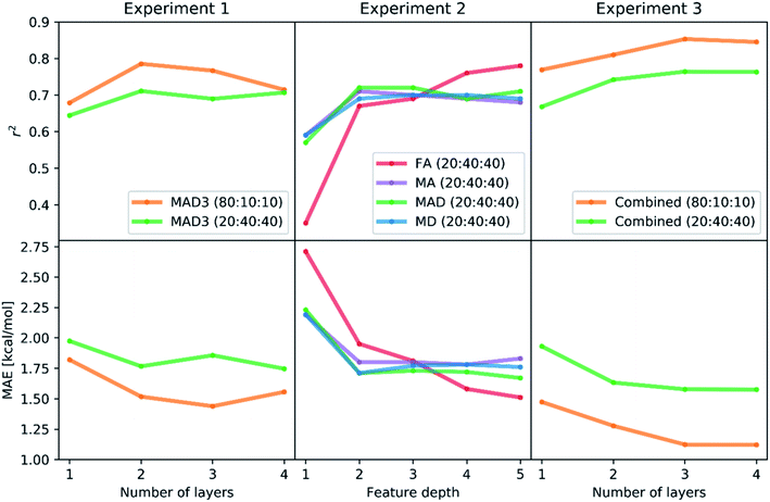
To estimate the performance of the autocorrelation-based catalyst representation in predicting activation barriers, we performed three numerical experiments with neural networks.104,109 In Experiment 1, we used the MAD3 representation (i.e. MAD features at depth = 3) and varied the fraction of data points used for training (20% and 80%) as well as the size of the artificial neural network. Training of neural networks only optimizes the adjustable weight parameters of the neural network that are used to pass information from layer to layer. The hyperparameters, such as the sizes of hidden layers, the dropout rate, and the L2 regularization parameter, have to be optimized manually without knowledge of gradients. There are multiple strategies for the optimization of hyperparameters, including grid search and random search (see Fig. 6A and B). In this work, we used a strategy pioneered by Adams et al.120 based on Bayesian optimization to determine the optimal hyperparameter values efficiently (see Fig. 6C). The main advantage of Bayesian optimization is that it achieves convergence with fewer calculations, though it has the drawback of running sequentially. Therefore, convergence may require longer computing times than trivially parallelizable methods such as grid and random searches. | ||
| Fig. 6 Optimization on a two-dimensional parameter space using (A) grid search, (B) random search and (C) Bayesian optimization-based (sequential) search. This approach has been pioneered by Adams et al. and is widely used to tune hyperparameters of ML models.120 | ||
The learning rate was dynamically adapted (decreased) during training to ensure optimal results. Prior tests showed that the rmsprop optimization method and relu activation functions lead to the best performing neural networks. The results of the hyperparameter Bayesian optimization for the minimization of the mean absolute error (MAE) are shown in Scheme 1 (Experiment 1, details in Tables S1 and S2‡†). We find the lowest MAEs (1.43 kcal mol−1 in case of 80% training fraction and 1.74 kcal mol−1 in case of 20% training fraction) when training with three or four hidden layers, while the most significant correlation coefficients r2 were already found with two hidden layers. It is possible that running the hyperparameter optimization to maximize r2 might also improve the results with three or four hidden layers.
The results of the Experiment 1 showed that three hidden layers is a sufficient depth to train neural networks with high accuracy. In case of a training fraction of 20%, the best performing model (MAE = 1.74 kcal mol−1) had four layers with 584, 94, 41 and 20 neurons, respectively, as well as an L2 parameter of 0.00044, a dropout rate of 1.62% and learning rate reduction after 29 epochs without validation loss decrease.
To compare the different representations described in the previous section, we performed Experiment 2, in which we only trained with a training–validation–test split of 20![[thin space (1/6-em)]](https://www.rsc.org/images/entities/char_2009.gif) :
:![[thin space (1/6-em)]](https://www.rsc.org/images/entities/char_2009.gif) 40
40![[thin space (1/6-em)]](https://www.rsc.org/images/entities/char_2009.gif) :
:![[thin space (1/6-em)]](https://www.rsc.org/images/entities/char_2009.gif) 40 and varied the input representations (FA, MA, MD, MAD, each from depth 1 to depth 5). Again, we used a Bayesian optimization-based hyperparameter optimization of the number of neurons in each layer, the dropout rate, and the L2 regularization parameter for each representation. We used the rmsprop optimizer and the relu activation. The best performing model is found when using FA features of up to depth 5 (FA5), with r2 = 0.78 and MAE = 1.51 kcal mol−1, followed by the MAD5 (1.67 kcal mol−1), MD5 (1.76 kcal mol−1) and MA5 (1.78 kcal mol−1) feature sets. The results of all models are presented in Scheme 1 (Experiment 2, details in Table S3‡†). The higher performance of the feature sets with larger maximum depth is not surprising as they yield a more unique description of each system, thus helping the model to distinguish similar complexes.
40 and varied the input representations (FA, MA, MD, MAD, each from depth 1 to depth 5). Again, we used a Bayesian optimization-based hyperparameter optimization of the number of neurons in each layer, the dropout rate, and the L2 regularization parameter for each representation. We used the rmsprop optimizer and the relu activation. The best performing model is found when using FA features of up to depth 5 (FA5), with r2 = 0.78 and MAE = 1.51 kcal mol−1, followed by the MAD5 (1.67 kcal mol−1), MD5 (1.76 kcal mol−1) and MA5 (1.78 kcal mol−1) feature sets. The results of all models are presented in Scheme 1 (Experiment 2, details in Table S3‡†). The higher performance of the feature sets with larger maximum depth is not surprising as they yield a more unique description of each system, thus helping the model to distinguish similar complexes.
To test whether the different representation methods tested in Experiment 2 complement each other or contain the same information, we did Experiment 3 where we merged all features into a single representation and again varied the training fraction as well as the neural network depth. We used training–validation–test splits of 80![[thin space (1/6-em)]](https://www.rsc.org/images/entities/char_2009.gif) :
:![[thin space (1/6-em)]](https://www.rsc.org/images/entities/char_2009.gif) 10
10![[thin space (1/6-em)]](https://www.rsc.org/images/entities/char_2009.gif) :
:![[thin space (1/6-em)]](https://www.rsc.org/images/entities/char_2009.gif) 10 and 20
10 and 20![[thin space (1/6-em)]](https://www.rsc.org/images/entities/char_2009.gif) :
:![[thin space (1/6-em)]](https://www.rsc.org/images/entities/char_2009.gif) 40
40![[thin space (1/6-em)]](https://www.rsc.org/images/entities/char_2009.gif) :
:![[thin space (1/6-em)]](https://www.rsc.org/images/entities/char_2009.gif) 40 and one to four hidden layers. In each case, we performed a Bayesian optimization-based hyperparameter optimization (neurons in each layer, learning rate, dropout, L2 regularization) and used the rmsprop optimizer, as well as the relu activation function. The results are shown in Scheme 1 (Experiment 3, details in Table S4‡†) with the best performing models having mean absolute errors of 1.12 kcal mol−1 in case of 80% training fraction (see Fig. 7A) and 1.58 kcal mol−1 in case of 20% training fraction (see Fig. 7B). It is worth noting the presence of strongly deviating points, though these are less than 1% of the total. These outliers might be associated to changes in the mechanism and/or DFT errors. A typical training curve of the neural network is shown in Fig. 7C, showing a decrease in training and validation loss as a function of the training epochs. The convergence of the training and validation losses and the small gap between them indicate that the neural network is not overfitting, which is achieved by using the Bayesian-optimized architecture and regularization (L2 and dropout) hyperparameters.
40 and one to four hidden layers. In each case, we performed a Bayesian optimization-based hyperparameter optimization (neurons in each layer, learning rate, dropout, L2 regularization) and used the rmsprop optimizer, as well as the relu activation function. The results are shown in Scheme 1 (Experiment 3, details in Table S4‡†) with the best performing models having mean absolute errors of 1.12 kcal mol−1 in case of 80% training fraction (see Fig. 7A) and 1.58 kcal mol−1 in case of 20% training fraction (see Fig. 7B). It is worth noting the presence of strongly deviating points, though these are less than 1% of the total. These outliers might be associated to changes in the mechanism and/or DFT errors. A typical training curve of the neural network is shown in Fig. 7C, showing a decrease in training and validation loss as a function of the training epochs. The convergence of the training and validation losses and the small gap between them indicate that the neural network is not overfitting, which is achieved by using the Bayesian-optimized architecture and regularization (L2 and dropout) hyperparameters.
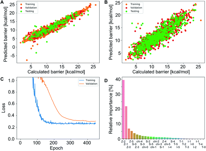 | ||
| Fig. 7 (A) Predictions of the best neural network models trained on 80% of the data points (4 layers, MAE = 1.12 kcal mol−1, r2 = 0.845; see Table S3‡†). (B) Predictions of the best neural network models trained on 20% of the data points (FA5 features, MAE = 1.51 kcal mol−1, r2 = 0.78; see Table S2‡†). (C) Loss of the neural network shown in panel (B) during training for the training and validation sets. (D) Feature importance of the same training data used in (B) determined using an independently trained gradient boosting regression model. | ||
The comparison of the performances of the neural networks trained in Experiment 3 on a combination of all feature sets to those of Experiment 2 indicates that all the information is already contained in the FA5 feature set (1.51 kcal mol−1 MAE with 20% training fraction). The addition of more features from other sets only increases the number of free parameters in the neural network and thus makes training and hyperparameter optimization more difficult (probably due to increased tendency to overfitting), which ultimately leads to worse results.
Fig. 7D shows an importance ranking of the FA5 features obtained by using a gradient boosting (GB) regression model (boosting steps = 100). We find that the five most essential features in the model predictions are Z-2, Z-5, χ-4, S-2, and χ-2. Composition, electronegativity, and size are thus more determining than the topology (T) and identity (I) features, which can be related to the higher impact of the former on chemical reactivity.
The lowest MAE (i.e. 1.12 kcal mol−1, see Fig. 7A) was obtained with an 80% training set and using the combination of all feature sets (FA, MA, MD, and MAD) at depth = 5, with a neural network containing four hidden layers. We will show in the next section that significantly lower errors can be reached by using Gaussian processes with a richer representation of Vaska's complexes including molecular fingerprints.
Small-data and explainable learning with Gaussian processes and gradient boosting regression
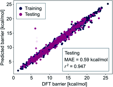
The observation that combining all feature-sets did not significantly improve model performance (i.e., comparing the results of Tables S3 and S4‡†) indicates that our optimized neural network models learn all the information contained in the autocorrelation feature sets. To obtain lower errors than those shown in the previous section, we have to improve the representation of the metal complexes to provide more information about their chemical structure to the machine learning models. Therefore, we extended the autocorrelation feature sets with chemical fingerprinting techniques. Molecular fingerprints are bit vectors in which each bit represents the presence of a particular molecular substructure of a given size, often called radius or depth. We generated RDKit (radius r1 and size s1) and circular Morgan (radius r2 and size s2) fingerprints121 of all complexes and appended them to the 20 autocorrelation features described above (FA3). These fingerprints, which can be easily computed in a laptop within seconds, facilitate the interpretation of the predictions by identifying specific molecular fragments (e.g. metal-bound ligands). For accurate prediction of activation energies, we then used a multistep process, including a gradient boosting (GB) model for feature selection based on importance, followed by a Gaussian process regression (GP) with the k most relevant features. The two-step procedure of feature selection followed by a Gaussian process model leads to improved results for the same reason as observed in Table S4‡† – having a too large amount of features can increase the complexity of the regression models in an unnecessary way which ultimately leads to worse performance, likely due to a limited number of kernels and thus hyperparameters used in the GP models.We found that r1 = 5, r2 = 3, s1 = s2 = 16![[thin space (1/6-em)]](https://www.rsc.org/images/entities/char_2009.gif) 384 and k = 300 lead to the highest prediction accuracy. The predictions of the best GP model, trained with 80% of the data, are shown in Fig. 8. Both the accuracy and the correlation of this model are very high, with MAE = 0.59 kcal mol−1 and r2 = 0.947.
384 and k = 300 lead to the highest prediction accuracy. The predictions of the best GP model, trained with 80% of the data, are shown in Fig. 8. Both the accuracy and the correlation of this model are very high, with MAE = 0.59 kcal mol−1 and r2 = 0.947.
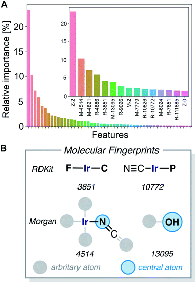
The gradient boosting (GB) model was also used to interpret the predictions. Fig. 9A shows the relative importance of the features, with the 15 most relevant highlighted in the inset. We found that the parameters Z-2, Z-0, chi-2, S-0, Z-3, S-3 and chi-3 of the 20D vector (FA3), as well as certain RDKit and Morgan fingerprint features, are contributing most to the predictions. We further analyzed the 20-dimensional feature vector and found that the four most important features are among the six features with the lowest correlation with any other of the features (Z-0, Z-1, Z-2, Z-3, χ-2, S-0), which makes them span a good basis for the 20-dimensional feature space. Pair–correlation plots of these features are shown in Fig. S5.‡†
The large fingerprint sizes of 4096 bits avoid hash collisions and thus allows us to analyze which molecular fragments (subgraphs of the molecule) activate these fingerprint features, which is illustrated for the four of the most important fingerprint features in Fig. 9B and S6.†
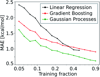
Due to the low number of free parameters compared to neural networks, Gaussian processes (GP) are models that are known to perform well in low data regimes.122 For that reason, we calculated the learning curve (i.e. test mean absolute error (MAE) as a function of training set size) of the GP model and compared it to that of the gradient boosting (GB; see Fig. 10). We find that the GP models outperform linear and gradient boosting regression models at all training fractions, leading to MAEs smaller than 1.0 kcal mol−1 already at low training fractions (0.1 to 0.2).
Additional calculations were carried out to explore the possibility of using a GP model trained on 80% of the data to enhance the convergence of the DFT calculations (Fig. 3). With this purpose, the GP model was retrained to predict the H–H distance at the transition state rather than the energy barrier. During the generation of the DFT data, 627 calculations failed due to convergence problems in the geometry optimizations. These calculations were reattempted by using an initial geometry guess of the TS in which the H–H distance was frozen at the value predicted by the GP model. With this ML-based protocol, 221 of the failed DFT calculations (i.e., 35%) were fully recovered, achieving convergence at all three stages (i.e.GEOM-1, TS-2 and COMPLEX-3). These results thus suggest that the GP models can be used iteratively to increase the size of the data sets used for training and testing.
Linking data-based knowledge and ML models to chemical interpretation
Being able to make predictions from a data-driven approach is a powerful asset. Nevertheless, such strategies can be shallow without chemical interpretability: it would be preferable to have a human-understandable model rather than it being used merely as a black-box.Our strategy takes chemical interpretability into consideration by three fronts: (1) with scatter plots of the extensive data set, we find how the H2-activation barriers correlate with different features (Fig. 4, S3 and S4†); (2) with gradient boosting regression, we learn what features are most important in the predictions (Fig. 9A); (3) with molecular fingerprints (Fig. 9B), we make a direct connection between the reactivity predicted for the Ir complexes and their structure. The last front is particularly appealing since it allows for analyzing steric and electronic effects with powerful tools like NBO analysis.
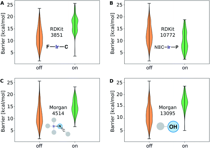
The structure–activity relationships are the most valuable and allow for complementing data-driven discovery with rational design strategies. Violin plots were used to represent the distribution of the energy barriers in the presence and absence of the ligands used to derive the chemical space from Vaska's complex. These plots are shown in Fig. 11 for a selection of ligands, including –F, –CN, –NCO/–NCS, and –OH. While –F, –NCO/–NCS, and –OH on average increase ΔE‡HH, the presence of the cyanide ligand on average decreases ΔE‡HH. These correlation directly links to the most relevant fingerprints identified in the gradient boosting regression model (Fig. 9B); e.g. the Morgan fingerprint 4514, which is nitrogen connected to Ir and a ![[double bond, length as m-dash]](https://www.rsc.org/images/entities/char_e001.gif) C
C![[double bond, length as m-dash]](https://www.rsc.org/images/entities/char_e001.gif) O or
O or ![[double bond, length as m-dash]](https://www.rsc.org/images/entities/char_e001.gif) C
C![[double bond, length as m-dash]](https://www.rsc.org/images/entities/char_e001.gif) S group, is associated with high H2-activation barriers. More importantly, it shows the influence of the ligand's π-donor/acceptor character on reactivity: strong π-donors (e.g. F; RDKit fingerprint 3851) slow down the reaction, whereas π-acceptors (e.g. CN; RDKit fingerprint 10772) accelerate it.
S group, is associated with high H2-activation barriers. More importantly, it shows the influence of the ligand's π-donor/acceptor character on reactivity: strong π-donors (e.g. F; RDKit fingerprint 3851) slow down the reaction, whereas π-acceptors (e.g. CN; RDKit fingerprint 10772) accelerate it.
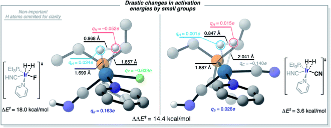
The understanding of the effect of each ligand in the H2-activation barrier is linked to the nature of the transition state. Vaska's complex and its derivatives activate H2 in a heterolytic fashion, almost as to forming a hydride and a proton at the TS in the most dramatic – and less efficient – case. This polarization of the breaking H–H bond is consistent with the ML models identifying the more electron-withdrawing ligands as those destabilizing the TS, and thus increasing ΔE‡HH, by introducing repulsive electrostatic interactions with the negatively-charged H-atom. This scenario is illustrated in Fig. 12 for the complex [Ir(PEt3)(Py)(CNH)(F)], with qH = −0.052e and qF = −0.639e. Fig. 12 also shows how the replacement of the F ligand by CN, which stabilizes a more electron-rich Ir center with its π-acceptor character, changes the nature of the interaction between the ligand (qC = −0.140e) and the H-atom (qH = 0.015e) from repulsive to attractive, thus lowering the ΔE‡HH barrier. This change from F to CN represents a difference in activation energies of 14.4 kcal mol−1, in favor of the more electron-accepting group. Overall, the results agree with the general trend of electron-rich metal centers promoting H2-activation by oxidative addition.
These effects are not hard to grasp and come naturally from our analysis based on gradient boosting and molecular fingerprints, showcasing the interpretability of our machine learning strategy. This strategy allows for the design of new metal species in the chemical space of Vaska's complex, with ample space for tuning the H2-activation rate.
Guidelines for model deployment
One potential use of the ML models reported herein is the discovery and optimization of catalysts based on transition metal complexes. In this section, we provide a few guidelines on how to follow this direction.The first step is to formulate the chemical space that will be explored. This chemical space is built by generalizing as much as possible the structure of a known or hypothetical catalyst. Factors like the trans influence of the ligands, their binding modes (e.g., κ1 or η2), and their preferred coordination isomers (e.g., cis or trans) can impact the scope of the final model and should thus be considered. Further, synthetic feasibility should be assessed together with the experimental collaborators.
The second step is to compute the features describing the whole chemical space. Based on the present work, the combination of autocorrelation functions with Morgan fingerprints is a good choice, with the latter allowing for the chemical interpretation of the predictions. The potential energy barrier of the key step in the catalysis is computed with a DFT method for a random selection of metal complexes. These energies will not be used to predict absolute experimental barriers, but rather to explore relative reactivity within the chemical space of the model. The computational cost should be moderate, allowing for the calculation of a significant amount of training data. If the key step is unknown, preliminary calculations and/or experiments will be required to clarify this point.
The third step is to train the ML model that will predict the energy barriers for all metal complexes in the chemical space. Based on the present work, Gaussian processes are a good choice because they can be trained with small data sets, yet achieving high accuracy in their predictions.
The fourth step is to select the complexes that will be tested in the lab. An initial selection is made based on the predictions of the ML model, picking those metal complexes that yield an optimal value of the key energy barrier. The preselected complexes are then filtered by high-level DFT calculations on the overall catalytic cycle, including thermodynamic and solvent effects, if relevant. The final pool of potential catalysts is then communicated to the experimentalists collaborators for its synthesis and testing.
Besides the protocol proposed above, the ML models should be carefully applied by considering these two limitations: 1. The models do not predict accurate values for energy barriers obtained with methods different from those used to compute the training data (e.g., experimental barriers from the literature, or barriers computed at a different level of theory); 2. The models do not predict mechanisms directly, but energy barriers (e.g., if a complex minimizes the barrier to a very small value, the rate of the catalytic process may then be determined by a different step). Both limitations highlight the importance of performing higher level calculations on the overall catalytic cycle to verify the catalysts selected by the ML models, before their experimental testing.
Conclusions
In this work, we provided an efficient protocol combining DFT and ML calculations for the prediction of reactivity in the oxidative addition of dihydrogen to iridium complexes. This broadly applicable protocol can, in principle, be adapted to cover different elementary steps, catalysts and/or substrates. Using an ample chemical space derived from Vaska's complex as a case study, we showed that the calculation of the H2-activation barrier (ΔE‡HH) at the DFT level can be automated and defined as the target to learn with ML models. Fingerprints, and autocorrelation and deltametric functions, were used and combined to compute sets of features representing each metal complex in the ML models. Besides these models, the substantial data set describing Vaska's complex region of the chemical space is valuable per se, and a simple analysis based on scatter plots showed interesting correlations providing chemical insight; e.g. increasing ΔE‡HH, with increasing |χ1| (i.e. electronegativity difference accounting for the polarization of the Ir–ligand bonds).Our work showed that ΔE‡HH can be predicted with high accuracy using ML models based on artificial neural network (ANN) and Gaussian process (GP) methods. Bayesian optimization (BO) proved to be an efficient approach to the optimization of the ANNs hyperparameters, including size, learning rate, and dropout and L2 regularization. The BO approach yielded highly accurate ANNs with both small (20%) and large (80%) training sets, avoiding overfitting and without delving into feature selection. By combining full- and metal-centered autocorrelation and deltametric functions, the lowest MAE achieved by the ANNs was 1.1 kcal mol−1 with an 80% training set.
We showed that accuracy can be further enhanced by using GP models trained with a set of selected features, including fingerprints. The lowest MAE achieved in this work, 0.6 kcal mol−1, was yielded by a GP model trained with an 80% training set. However, the most valuable asset of the GP models is the possibility of minimizing the MAE below 1 kcal mol−1 with minimal training sets containing 20% or less of the data available. i.e., After computing the energy barrier for a few hundred metal complexes, accurate predictions can be made over thousands.
Further, we showed that gradient boosting (GB) regression can be used to select the features of the GP models and to interpret the predictions – both tasks are based on the calculation of the importance of the features. For the autocorrelation and deltametric features, the GB models showed that chemical composition and atom size and electronegativity have a stronger impact on the H2-activation barriers than other features accounting for topology and size in number of atoms. The relevance of the fingerprints in the predictions provided further insight into the structure–activity relationships of the system by identifying ligands (and ligand fragments) that either heighten (e.g. F) or lower (e.g. CN) the H2-activation barrier.
In summary, we proved a high-throughput virtual screening approach in which synthetic data from DFT calculations are used to build ML models predicting the reactivity of metal complexes. This approach is based on a novel combination of existing methods, including affordable descriptors and state-of-the-art ML models. In particular, GP models are especially appealing because small amounts of DFT data are enough to achieve MAE < 1 kcal mol−1 in the prediction of energy barriers. These models are speedy (i.e. minutes on a laptop or PC) and thus allow for the exploration of large chemical spaces and the discovery of new metal complexes with optimal reactivity properties, which is one of the holy grails in the field of catalysis. The approach reported herein can be applied to other reactions of high interest, including water oxidation and CO2 reduction.
Methods
DFT
All DFT calculations were carried out with the Gaussian09 program at the PBE/def2-SVP level,123,124 including dispersion corrections with the Grimme's D3 model.125 The ultrafine pruned (99![[thin space (1/6-em)]](https://www.rsc.org/images/entities/char_2009.gif) 590) grid was used for higher numerical accuracy and stability. Geometry optimizations were performed in the gas phase. Overall, 7722 DFT calculations (i.e., 2574 × 3) where performed on a parallel supercomputer, by using 16 CPU-cores for each job and by distributing multi-job tasks over several computing nodes. After the first run, many calculations failed to converge, mostly at the GEOM-1 and COMPLEX-3 stages. The number of failures was significant, yielding a rather low success rate in the calculation of the H2-activation barriers (59%). The analysis of the output files revealed that most jobs failed due to an error either in the geometry constraints (GEOM-1) or in the minimization of the gradient (COMPLEX-3). These errors were tackled in an automated manner, increasing the overall success rate to 85% (i.e., 2197 systems converged). The failures in geometry optimization appeared to be mostly related to the quality of the initial guess. In line with this, convergence was enhanced upon using TS metrics (i.e., breaking H⋯H distance) predicted by ML models. All calculations were carried out for the neutral singlet state.
590) grid was used for higher numerical accuracy and stability. Geometry optimizations were performed in the gas phase. Overall, 7722 DFT calculations (i.e., 2574 × 3) where performed on a parallel supercomputer, by using 16 CPU-cores for each job and by distributing multi-job tasks over several computing nodes. After the first run, many calculations failed to converge, mostly at the GEOM-1 and COMPLEX-3 stages. The number of failures was significant, yielding a rather low success rate in the calculation of the H2-activation barriers (59%). The analysis of the output files revealed that most jobs failed due to an error either in the geometry constraints (GEOM-1) or in the minimization of the gradient (COMPLEX-3). These errors were tackled in an automated manner, increasing the overall success rate to 85% (i.e., 2197 systems converged). The failures in geometry optimization appeared to be mostly related to the quality of the initial guess. In line with this, convergence was enhanced upon using TS metrics (i.e., breaking H⋯H distance) predicted by ML models. All calculations were carried out for the neutral singlet state.
ML
We used TensorFlow126 to train the neural networks. We used RDKit to generate the RDKit and Morgan fingerprints. We used the gradient boosting regression method127 implemented in scikit-learn and the Gaussian Process method implemented in gpflow.128 The GP model was trained with the white noise and radial basis function (RBF) kernels for the selected features of the 20D vector, the RDKit fingerprints, and the Morgan fingerprints, respectively. All FA, MA, MD, and MAD features were computed with the molSimplify library developed by Kulik and coworkers.119 The data were randomly splitted into training, validation and testing sets of variable size, with the aim of determining the effect of the latter on accuracy.Conflicts of interest
There are no conflicts to declare.Acknowledgements
P. F. has received funding from the European Union's Horizon 2020 research and innovation program under the Marie Sklodowska-Curie grant agreement no. 795206. We thank Compute Canada for the computational resources. A. A.-G. thanks Anders G. Frøseth for his generous support. A. A.-G. also acknowledges the generous support of Natural Resources Canada and the Canada 150 Research Chairs program. D. B. acknowledges the support of the Research Council of Norway through its Centers of Excellence Scheme (project number 262695) and the Norwegian Metacenter for Computational Science (NOTUR; project nn4654k). ML computations were made on the supercomputer “beluga” from École de technologie supérieure, managed by Calcul Québec and Compute Canada. The operation of this supercomputer is funded by the Canada Foundation for Innovation (CFI), the Ministère de l'Économie, de la Science et de l'Innovation du Québec (MESI) and the Fonds de recherche du Québec – Nature et technologies (FRQ-NT).References
- M. D. Kärkäs, O. Verho, E. V. Johnston and B. Åkermark, Artificial Photosynthesis: Molecular Systems for Catalytic Water Oxidation, Chem. Rev., 2014, 114(24), 11863–12001, DOI:10.1021/cr400572f.
- R. Matheu, M. Z. Ertem, C. Gimbert-Suriñach, X. Sala and A. Llobet, Seven Coordinated Molecular Ruthenium–Water Oxidation Catalysts: A Coordination Chemistry Journey, Chem. Rev., 2019, 119(6), 3453–3471, DOI:10.1021/acs.chemrev.8b00537.
- J. D. Blakemore, R. H. Crabtree and G. W. Brudvig, Molecular Catalysts for Water Oxidation, Chem. Rev., 2015, 115(23), 12974–13005, DOI:10.1021/acs.chemrev.5b00122.
- T. J. Meyer, M. V. Sheridan and B. D. Sherman, Mechanisms of Molecular Water Oxidation in Solution and on Oxide Surfaces, Chem. Soc. Rev., 2017, 46(20), 6148–6169, 10.1039/C7CS00465F.
- N. Cox, D. A. Pantazis, F. Neese and W. Lubitz, Biological Water Oxidation, Acc. Chem. Res., 2013, 46(7), 1588–1596, DOI:10.1021/ar3003249.
- L. Duan, L. Wang, F. Li, F. Li and L. Sun, Highly Efficient Bioinspired Molecular Ru Water Oxidation Catalysts with Negatively Charged Backbone Ligands, Acc. Chem. Res., 2015, 48(7), 2084–2096, DOI:10.1021/acs.accounts.5b00149.
- D. W. Shaffer, Y. Xie and J. J. Concepcion, O–O Bond Formation in Ruthenium-Catalyzed Water Oxidation: Single-Site Nucleophilic Attack vs. O–O Radical Coupling, Chem. Soc. Rev., 2017, 46(20), 6170–6193, 10.1039/C7CS00542C.
- W.-H. Wang, Y. Himeda, J. T. Muckerman, G. F. Manbeck and E. Fujita, CO2 Hydrogenation to Formate and Methanol as an Alternative to Photo- and Electrochemical CO2 Reduction, Chem. Rev., 2015, 115(23), 12936–12973, DOI:10.1021/acs.chemrev.5b00197.
- W. Wang, S. Wang, X. Ma and J. Gong, Recent Advances in Catalytic Hydrogenation of Carbon Dioxide, Chem. Soc. Rev., 2011, 3703–3727, 10.1039/c1cs15008a.
- M. Rakowski Dubois and D. L. Dubois, Development of Molecular Electrocatalysts for CO2 Reduction and H2 Production/Oxidation, Acc. Chem. Res., 2009, 42(12), 1974–1982, DOI:10.1021/ar900110c.
- A. J. Morris, G. J. Meyer and E. Fujita, Molecular Approaches to the Photocatalytic Reduction of Carbon Dioxide for Solar Fuels, Acc. Chem. Res., 2009, 42(12), 1983–1994, DOI:10.1021/ar9001679.
- C. Costentin, M. Robert and J.-M. Savéant, Catalysis of the Electrochemical Reduction of Carbon Dioxide, Chem. Soc. Rev., 2013, 42(6), 2423–2436, 10.1039/C2CS35360A.
- D. Balcells, E. Clot and O. Eisenstein, C—H Bond Activation in Transition Metal Species from a Computational Perspective, Chem. Rev., 2010, 110(2), 749–823, DOI:10.1021/cr900315k.
- D. Balcells and F. Maseras, Computational Approaches to Asymmetric Synthesis, New J. Chem., 2007, 31(3), 333–343, 10.1039/B615528F.
- P. Vidossich, A. Lledós and G. Ujaque, First-Principles Molecular Dynamics Studies of Organometallic Complexes and Homogeneous Catalytic Processes, Acc. Chem. Res., 2016, 49(6), 1271–1278, DOI:10.1021/acs.accounts.6b00054.
- S. Ahn, M. Hong, M. Sundararajan, D. H. Ess and M.-H. Baik, Design and Optimization of Catalysts Based on Mechanistic Insights Derived from Quantum Chemical Reaction Modeling, Chem. Rev., 2019, 119(11), 6509–6560, DOI:10.1021/acs.chemrev.9b00073.
- D. L. Davies, S. A. Macgregor and C. L. McMullin, Computational Studies of Carboxylate-Assisted C–H Activation and Functionalization at Group 8–10 Transition Metal Centers, Chem. Rev., 2017, 117(13), 8649–8709, DOI:10.1021/acs.chemrev.6b00839.
- M. García-Melchor, A. A. C. Braga, A. Lledós, G. Ujaque and F. Maseras, Computational Perspective on Pd-Catalyzed C–C Cross-Coupling Reaction Mechanisms, Acc. Chem. Res., 2013, 46(11), 2626–2634, DOI:10.1021/ar400080r.
- J. N. Harvey, F. Himo, F. Maseras and L. Perrin, Scope and Challenge of Computational Methods for Studying Mechanism and Reactivity in Homogeneous Catalysis, ACS Catal., 2019, 9(8), 6803–6813, DOI:10.1021/acscatal.9b01537.
- L. Noodleman, T. Lovell, W.-G. Han, J. Li and F. Himo, Quantum Chemical Studies of Intermediates and Reaction Pathways in Selected Enzymes and Catalytic Synthetic Systems, Chem. Rev., 2004, 104(2), 459–508, DOI:10.1021/cr020625a.
- M. Obst, L. Pavlovic and K. H. Hopmann, Carbon-Carbon Bonds with CO2: Insights from Computational Studies, J. Organomet. Chem., 2018, 864, 115–127 CrossRef CAS.
- T. Sperger, I. A. Sanhueza, I. Kalvet and F. Schoenebeck, Computational Studies of Synthetically Relevant Homogeneous Organometallic Catalysis Involving Ni, Pd, Ir, and Rh: An Overview of Commonly Employed DFT Methods and Mechanistic Insights, Chem. Rev., 2015, 115(17), 9532–9586, DOI:10.1021/acs.chemrev.5b00163.
- J. L. Reymond, The Chemical Space Project, Acc. Chem. Res., 2015, 48(3), 722–730, DOI:10.1021/ar500432k.
- D. J. Durand and N. Fey, Computational Ligand Descriptors for Catalyst Design, Chem. Rev., 2019, 119(11), 6561–6594, DOI:10.1021/acs.chemrev.8b00588.
- N. Fey, Lost in Chemical Space? Maps to Support Organometallic Catalysis, Chem. Cent. J., 2015, 9(1), 38, DOI:10.1186/s13065-015-0104-5.
- D. W. Robbins and J. F. Hartwig, A Simple, Multidimensional Approach to High-Throughput Discovery of Catalytic Reactions, Science, 2011, 333(6048), 1423, DOI:10.1126/science.1207922.
- S. M. Preshlock, B. Ghaffari, P. E. Maligres, S. W. Krska, R. E. Maleczka and M. R. Smith, High-Throughput Optimization of Ir-Catalyzed C–H Borylation: A Tutorial for Practical Applications, J. Am. Chem. Soc., 2013, 135(20), 7572–7582, DOI:10.1021/ja400295v.
- M. S. Eom, J. Noh, H.-S. Kim, S. Yoo, M. S. Han and S. Lee, High-Throughput Screening Protocol for the Coupling Reactions of Aryl Halides Using a Colorimetric Chemosensor for Halide Ions, Org. Lett., 2016, 18(8), 1720–1723, DOI:10.1021/acs.orglett.6b00300.
- K. D. Collins, T. Gensch and F. Glorius, Contemporary Screening Approaches to Reaction Discovery and Development, Nat. Chem., 2014, 6, 859, DOI:10.1038/nchem.2062.
- V. L. Cruz, S. Martinez, J. Ramos and J. Martinez-Salazar, 3D-QSAR as a Tool for Understanding and Improving Single-Site Polymerization Catalysts. A Review, Organometallics, 2014, 33(12), 2944–2959, DOI:10.1021/om400721v.
- A. G. Maldonado and G. Rothenberg, Predictive Modeling in Homogeneous Catalysis: A Tutorial, Chem. Soc. Rev., 2010, 39(6), 1891–1902, 10.1039/B921393G.
- J. A. Hageman, J. A. Westerhuis, H.-W. Frühauf and G. Rothenberg, Design and Assembly of Virtual Homogeneous Catalyst Libraries –Towards in Silico Catalyst Optimisation, Adv. Synth. Catal., 2006, 348(3), 361–369, DOI:10.1002/adsc.200505299.
- E. Burello and G. Rothenberg, In Silico Design in Homogeneous Catalysis Using Descriptor Modelling, Int. J. Mol. Sci., 2006, 7(9), 375–404 CrossRef CAS.
- E. Burello, D. Farrusseng and G. Rothenberg, Combinatorial Explosion in Homogeneous Catalysis: Screening 60,000 Cross-Coupling Reactions, Adv. Synth. Catal., 2004, 346(13–15), 1844–1853, DOI:10.1002/adsc.200404170.
- K. Wu and A. G. Doyle, Parameterization of Phosphine Ligands Demonstrates Enhancement of Nickel Catalysis via Remote Steric Effects, Nat. Chem., 2017, 9, 779, DOI:10.1038/nchem.2741.
- M. S. Sigman, K. C. Harper, E. N. Bess and A. Milo, The Development of Multidimensional Analysis Tools for Asymmetric Catalysis and Beyond, Acc. Chem. Res., 2016, 49(6), 1292–1301, DOI:10.1021/acs.accounts.6b00194.
- C. B. Santiago, J.-Y. Guo and M. S. Sigman, Predictive and Mechanistic Multivariate Linear Regression Models for Reaction Development, Chem. Sci., 2018, 9(9), 2398–2412, 10.1039/C7SC04679K.
- Z. L. Niemeyer, A. Milo, D. P. Hickey and M. S. Sigman, Parameterization of Phosphine Ligands Reveals Mechanistic Pathways and Predicts Reaction Outcomes, Nat. Chem., 2016, 8, 610, DOI:10.1038/nchem.2501.
- K. C. Harper and M. S. Sigman, Three-Dimensional Correlation of Steric and Electronic Free Energy Relationships Guides Asymmetric Propargylation, Science, 2011, 333(6051), 1875, DOI:10.1126/science.1206997.
- A. R. Rosales, J. Wahlers, E. Limé, R. E. Meadows, K. W. Leslie, R. Savin, F. Bell, E. Hansen, P. Helquist, R. H. Munday, O. Wiest and P.-O. Norrby, Rapid Virtual Screening of Enantioselective Catalysts Using CatVS, Nat. Catal., 2019, 2(1), 41–45, DOI:10.1038/s41929-018-0193-3.
- D.-H. Kwon, J. T. Fuller, U. J. Kilgore, O. L. Sydora, S. M. Bischof and D. H. Ess, Computational Transition-State Design Provides Experimentally Verified Cr(P,N) Catalysts for Control of Ethylene Trimerization and Tetramerization, ACS Catal., 2018, 8(2), 1138–1142, DOI:10.1021/acscatal.7b04026.
- R. Fu, R. J. Nielsen, W. A. Goddard, G. C. Fortman and T. B. Gunnoe, DFT Virtual Screening Identifies Rhodium–Amidinate Complexes As Potential Homogeneous Catalysts for Methane-to-Methanol Oxidation, ACS Catal., 2014, 4(12), 4455–4465, DOI:10.1021/cs5005322.
- Y. Chu, W. Heyndrickx, G. Occhipinti, V. R. Jensen and B. K. Alsberg, An Evolutionary Algorithm for de Novo Optimization of Functional Transition Metal Compounds, J. Am. Chem. Soc., 2012, 134(21), 8885–8895, DOI:10.1021/ja300865u.
- B. J. Rooks, M. R. Haas, D. Sepúlveda, T. Lu and S. E. Wheeler, Prospects for the Computational Design of Bipyridine N,N′-Dioxide Catalysts for Asymmetric Propargylation Reactions, ACS Catal., 2015, 5(1), 272–280, DOI:10.1021/cs5012553.
- J. G. Freeze, H. R. Kelly and V. S. Batista, Search for Catalysts by Inverse Design: Artificial Intelligence, Mountain Climbers, and Alchemists, Chem. Rev., 2019, 119(11), 6595–6612, DOI:10.1021/acs.chemrev.8b00759.
- R. Gómez-Bombarelli, J. N. Wei, D. Duvenaud, J. M. Hernández-Lobato, B. Sánchez-Lengeling, D. Sheberla, J. Aguilera-Iparraguirre, T. D. Hirzel, R. P. Adams and A. Aspuru-Guzik, Automatic Chemical Design Using a Data-Driven Continuous Representation of Molecules, ACS Cent. Sci., 2018, 4(2), 268–276, DOI:10.1021/acscentsci.7b00572.
- M. Popova, O. Isayev and A. Tropsha, Deep Reinforcement Learning for de Novo Drug Design, Sci. Adv., 2018, 4(7), eaap7885, DOI:10.1126/sciadv.aap7885.
- B. Sanchez-Lengeling and A. Aspuru-Guzik, Inverse Molecular Design Using Machine Learning: Generative Models for Matter Engineering, Science, 2018, 361(6400), 360, DOI:10.1126/science.aat2663.
- B. Sanchez-Lengeling, C. Outeiral, G. L. Guimaraes and A. Aspuru-Guzik, Optimizing Distributions over Molecular Space. An Objective-Reinforced Generative Adversarial Network for Inverse-Design Chemistry (ORGANIC), DOI:10.26434/CHEMRXIV.5309668.V3.
- D. Schwalbe-Koda and R. Gómez-Bombarelli, Generative Models for Automatic Chemical Design, 2019, arXiv:1907.01632.
- P. S. Gromski, A. B. Henson, J. M. Granda and L. Cronin, How to Explore Chemical Space Using Algorithms and Automation, Nat. Rev. Chem., 2019, 3(2), 119–128, DOI:10.1038/s41570-018-0066-y.
- K. T. Butler, D. W. Davies, H. Cartwright, O. Isayev and A. Walsh, Machine Learning for Molecular and Materials Science, Nature, 2018, 559(7715), 547–555, DOI:10.1038/s41586-018-0337-2.
- A. P. Bartok, S. De, C. Poelking, N. Bernstein, J. R. Kermode, G. Csanyi and M. Ceriotti, Machine Learning Unifies the Modeling of Materials and Molecules, Sci. Adv., 2017, 3(12), 8, DOI:10.1126/sciadv.1701816.
- P. Raccuglia, K. C. Elbert, P. D. F. Adler, C. Falk, M. B. Wenny, A. Mollo, M. Zeller, S. A. Friedler, J. Schrier and A. J. Norquist, Machine-Learning-Assisted Materials Discovery Using Failed Experiments, Nature, 2016, 533, 73, DOI:10.1038/nature17439.
- T. C. Le and D. A. Winkler, Discovery and Optimization of Materials Using Evolutionary Approaches, Chem. Rev., 2016, 116(10), 6107–6132, DOI:10.1021/acs.chemrev.5b00691.
- R. Gomez-Bombarelli, J. Aguilera-Iparraguirre, T. D. Hirzel, D. Duvenaud, D. Maclaurin, M. A. Blood-Forsythe, H. S. Chae, M. Einzinger, D. G. Ha, T. Wu, G. Markopoulos, S. Jeon, H. Kang, H. Miyazaki, M. Numata, S. Kim, W. Huang, S. I. Hong, M. Baldo, R. P. Adams and A. Aspuru-Guzik, Design of Efficient Molecular Organic Light-Emitting Diodes by a High-Throughput Virtual Screening and Experimental Approach, Nat. Mater., 2016, 15(10), 1120–1127, DOI:10.1038/nmat4717.
- Z. Jensen, E. Kim, S. Kwon, T. Z. H. Gani, Y. Román-Leshkov, M. Moliner, A. Corma and E. Olivetti, A Machine Learning Approach to Zeolite Synthesis Enabled by Automatic Literature Data Extraction, ACS Cent. Sci., 2019, 5(5), 892–899, DOI:10.1021/acscentsci.9b00193.
- Y. J. Colón and R. Q. Snurr, High-Throughput Computational Screening of Metal–Organic Frameworks, Chem. Soc. Rev., 2014, 43(16), 5735–5749, 10.1039/C4CS00070F.
- M. Fernandez, P. G. Boyd, T. D. Daff, M. Z. Aghaji and T. K. Woo, Rapid and Accurate Machine Learning Recognition of High Performing Metal Organic Frameworks for CO2 Capture, J. Phys. Chem. Lett., 2014, 5(17), 3056–3060, DOI:10.1021/jz501331m.
- B. Meredig, A. Agrawal, S. Kirklin, J. E. Saal, J. W. Doak, A. Thompson, K. Zhang, A. Choudhary and C. Wolverton, Combinatorial Screening for New Materials in Unconstrained Composition Space with Machine Learning, Phys. Rev. B, 2014, 89(9), 7, DOI:10.1103/PhysRevB.89.094104.
- E. O. Pyzer-Knapp, K. Li and A. Aspuru-Guzik, Learning from the Harvard Clean Energy Project: The Use of Neural Networks to Accelerate Materials Discovery, Adv. Funct. Mater., 2015, 25(41), 6495–6502, DOI:10.1002/adfm.201501919.
- H. Altae-Tran, B. Ramsundar, A. S. Pappu and V. Pande, Low Data Drug Discovery with One-Shot Learning, ACS Cent. Sci., 2017, 3(4), 283–293, DOI:10.1021/acscentsci.6b00367.
- G. Schneider and D. E. Clark, Automated De Novo Drug Design: Are We Nearly There Yet?, Angew. Chem., Int. Ed., 2019, 58(32), 10792–10803, DOI:10.1002/anie.201814681.
- H. M. Chen, O. Engkvist, Y. H. Wang, M. Olivecrona and T. Blaschke, The Rise of Deep Learning in Drug Discovery, Drug Discovery Today, 2018, 23(6), 1241–1250, DOI:10.1016/j.drudis.2018.01.039.
- A. Lavecchia, Machine-Learning Approaches in Drug Discovery: Methods and Applications, Drug Discovery Today, 2015, 20(3), 318–331, DOI:10.1016/j.drudis.2014.10.012.
- Y. C. Lo, S. E. Rensi, W. Torng and R. B. Altman, Machine Learning in Chemoinformatics and Drug Discovery, Drug Discovery Today, 2018, 23(8), 1538–1546, DOI:10.1016/j.drudis.2018.05.010.
- A. Mayr, G. Klambauer, T. Unterthiner, M. Steijaert, J. K. Wegner, H. Ceulemans, D. A. Clevert and S. Hochreiter, Large-Scale Comparison of Machine Learning Methods for Drug Target Prediction on ChEMBL, Chem. Sci., 2018, 9(24), 5441–5451, 10.1039/c8sc00148k.
- P. Mamoshina, A. Vieira, E. Putin and A. Zhavoronkov, Applications of Deep Learning in Biomedicine, Mol. Pharm., 2016, 13(5), 1445–1454, DOI:10.1021/acs.molpharmaceut.5b00982.
- J. M. Granda, L. Donina, V. Dragone, D.-L. Long and L. Cronin, Controlling an Organic Synthesis Robot with Machine Learning to Search for New Reactivity, Nature, 2018, 559(7714), 377–381, DOI:10.1038/s41586-018-0307-8.
- B. Liu, B. Ramsundar, P. Kawthekar, J. Shi, J. Gomes, Q. Luu Nguyen, S. Ho, J. Sloane, P. Wender and V. Pande, Retrosynthetic Reaction Prediction Using Neural Sequence-to-Sequence Models, ACS Cent. Sci., 2017, 3(10), 1103–1113, DOI:10.1021/acscentsci.7b00303.
- B. Maryasin, P. Marquetand and N. Maulide, Machine Learning for Organic Synthesis: Are Robots Replacing Chemists?, Angew. Chem., Int. Ed., 2018, 57(24), 6978–6980, DOI:10.1002/anie.201803562.
- M. H. S. Segler, M. Preuss and M. P. Waller, Planning Chemical Syntheses with Deep Neural Networks and Symbolic AI, Nature, 2018, 555(7698), 604–610, DOI:10.1038/nature25978.
- C. W. Coley, W. H. Green and K. F. Jensen, Machine Learning in Computer-Aided Synthesis Planning, Acc. Chem. Res., 2018, 51(5), 1281–1289, DOI:10.1021/acs.accounts.8b00087.
- J. Wellendorff, K. T. Lundgaard, A. Mogelhoj, V. Petzold, D. D. Landis, J. K. Norskov, T. Bligaard and K. W. Jacobsen, Density Functionals for Surface Science: Exchange-Correlation Model Development with Bayesian Error Estimation, Phys. Rev. B, 2012, 85(23), 23, DOI:10.1103/PhysRevB.85.235149.
- J. Behler, Perspective: Machine Learning Potentials for Atomistic Simulations, J. Chem. Phys., 2016, 145(17), 9, DOI:10.1063/1.4966192.
- Z. W. Li, J. R. Kermode and A. De Vita, Molecular Dynamics with On-the-Fly Machine Learning of Quantum-Mechanical Forces, Phys. Rev. Lett., 2015, 114(9), 5, DOI:10.1103/PhysRevLett.114.096405.
- J. C. Snyder, M. Rupp, K. Hansen, K. R. Muller and K. Burke, Finding Density Functionals with Machine Learning, Phys. Rev. Lett., 2012, 108(25), 5, DOI:10.1103/PhysRevLett.108.253002.
- J. Wang, S. Olsson, C. Wehmeyer, A. Perez, N. E. Charron, G. de Fabritiis, F. Noe and C. Clementi, Machine Learning of Coarse-Grained Molecular Dynamics Force Fields, ACS Cent. Sci., 2019, 5(5), 755–767, DOI:10.1021/acscentsci.8b00913.
- M. Rupp, A. Tkatchenko, K. R. Muller and O. A. von Lilienfeld, Fast and Accurate Modeling of Molecular Atomization Energies with Machine Learning, Phys. Rev. Lett., 2012, 108(5), 5, DOI:10.1103/PhysRevLett.108.058301.
- C. R. Duan, J. P. Janet, F. Liu, A. Nandy and H. J. Kulik, Learning from Failure: Predicting Electronic Structure Calculation Outcomes with Machine Learning Models, J. Chem. Theory Comput., 2019, 15(4), 2331–2345, DOI:10.1021/acs.jctc.9b00057.
- M. Gastegger, J. Behler and P. Marquetand, Machine Learning Molecular Dynamics for the Simulation of Infrared Spectra, Chem. Sci., 2017, 8(10), 6924–6935, 10.1039/c7sc02267k.
- A. Nandy, C. R. Duan, J. P. Janet, S. Gugler and H. J. Kulik, Strategies and Software for Machine Learning Accelerated Discovery in Transition Metal Chemistry, Ind. Eng. Chem. Res., 2018, 57(42), 13973–13986, DOI:10.1021/acs.iecr.8b04015.
- J. P. Janet, F. Liu, A. Nandy, C. R. Duan, T. H. Yang, S. Lin and H. J. Kulik, Designing in the Face of Uncertainty: Exploiting Electronic Structure and Machine Learning Models for Discovery in Inorganic Chemistry, Inorg. Chem., 2019, 58(16), 10592–10606, DOI:10.1021/acs.inorgchem.9b00109.
- J. R. Kitchin, Machine Learning in Catalysis, Nat. Catal., 2018, 1(4), 230–232, DOI:10.1038/s41929-018-0056-y.
- Z. Li, S. W. Wang and H. L. Xin, Toward Artificial Intelligence in Catalysis, Nat. Catal., 2018, 1(9), 641–642, DOI:10.1038/s41929-018-0150-1.
- L. A. Baumes, J. M. Serra, P. Serna and A. Corma, Support Vector Machines for Predictive Modeling in Heterogeneous Catalysis: A Comprehensive Introduction and Overfitting Investigation Based on Two Real Applications, J. Comb. Chem., 2006, 8(4), 583–596, DOI:10.1021/cc050093m.
- B. R. Goldsmith, J. Esterhuizen, J. X. Liu, C. J. Bartel and C. Sutton, Machine Learning for Heterogeneous Catalyst Design and Discovery, AIChE J., 2018, 64(7), 2311–2323, DOI:10.1002/aic.16198.
- L. Grajciar, C. J. Heard, A. A. Bondarenko, M. V. Polynski, J. Meeprasert, E. A. Pidko and P. Nachtigall, Towards Operando Computational Modeling in Heterogeneous Catalysis, Chem. Soc. Rev., 2018, 47(22), 8307–8348, 10.1039/c8cs00398j.
- O. Mamun, K. T. Winther, J. R. Boes and T. Bligaard, High-Throughput Calculations of Catalytic Properties of Bimetallic Alloy Surfaces, Sci. Data, 2019, 6, 9, DOI:10.1038/s41597-019-0080-z.
- J. Ohyama, S. Nishimura and K. Takahashi, Data Driven Determination of Reaction Conditions in Oxidative Coupling of Methane via Machine Learning, ChemCatChem, 2019, 11, 4307–4313, DOI:10.1002/cctc.201900843.
- K. Tran and Z. W. Ulissi, Active Learning across Intermetallics to Guide Discovery of Electrocatalysts for CO2 Reduction and H2 Evolution, Nat. Catal., 2018, 1(9), 696–703, DOI:10.1038/s41929-018-0142-1.
- A. R. Singh, B. A. Rohr, J. A. Gauthier and J. K. Norskov, Predicting Chemical Reaction Barriers with a Machine Learning Model, Catal. Lett., 2019, 149(9), 2347–2354, DOI:10.1007/s10562-019-02705-x.
- Z. W. Ulissi, M. T. Tang, J. P. Xiao, X. Y. Liu, D. A. Torelli, M. Karamad, K. Cummins, C. Hahn, N. S. Lewis, T. F. Jaramillo, K. Chan and J. K. Nørskov, Machine-Learning Methods Enable Exhaustive Searches for Active Bimetallic Facets and Reveal Active Site Motifs for CO2 Reduction, ACS Catal., 2017, 7(10), 6600–6608, DOI:10.1021/acscatal.7b01648.
- (a) A. F. Zahrt, J. J. Henle, B. T. Rose, Y. Wang, W. T. Darrow and S. E. Denmark, Prediction of Higher-Selectivity Catalysts by Computer-Driven Workflow and Machine Learning, Science, 2019, 363, eaau5631, DOI:10.1126/science.aau5631; (b) A. F. Zahrt, S. V. Athavale and S. E. Denmark, Quantitative Structure–Selectivity Relationships in Enantioselective Catalysis: Past, Present, and Future, Chem. Rev., 2020, 120, 1620, DOI:10.1021/acs.chemrev.9b00425.
- S. Banerjee, A. Sreenithya and R. B. Sunoj, Machine Learning for Predicting Product Distributions in Catalytic Regioselective Reactions, Phys. Chem. Chem. Phys., 2018, 20(27), 18311–18318, 10.1039/C8CP03141J.
- Y. Amar, A. Schweidtmann, P. Deutsch, L. W. Cao and A. Lapkin, Machine Learning and Molecular Descriptors Enable Rational Solvent Selection in Asymmetric Catalysis, Chem. Sci., 2019, 10(27), 6697–6706, 10.1039/c9sc01844a.
- D. T. Ahneman, J. G. Estrada, S. S. Lin, S. D. Dreher and A. G. Doyle, Predicting Reaction Performance in C-N Cross-Coupling Using Machine Learning, Science, 2018, 360(6385), 186–190, DOI:10.1126/science.aar5169.
- B. Meyer, B. Sawatlon, S. Heinen, O. A. Von Lilienfeld and C. Corminboeuf, Machine Learning Meets Volcano Plots: Computational Discovery of Cross-Coupling Catalysts, Chem. Sci., 2018, 9(35), 7069–7077, 10.1039/c8sc01949e.
- S. Back, K. Tran and Z. W. Ulissi, Toward a Design of Active Oxygen Evolution Catalysts: Insights from Automated Density Functional Theory Calculations and Machine Learning, ACS Catal., 2019, 7651–7659, DOI:10.1021/acscatal.9b02416.
- A. Jinich, B. Sanchez-Lengeling, H. Ren, R. Harman and A. Aspuru-Guzik, A Mixed Quantum Chemistry/Machine Learning Approach for the Fast and Accurate Prediction of Biochemical Redox Potentials and Its Large-Scale Application to 315 000 Redox Reactions, ACS Cent. Sci., 2019, 5(7), 1199–1210, DOI:10.1021/acscentsci.9b00297.
- P. Sadowski, D. Fooshee, N. Subrahmanya and P. Baldi, Synergies Between Quantum Mechanics and Machine Learning in Reaction Prediction, J. Chem. Inf. Model., 2016, 56(11), 2125–2128, DOI:10.1021/acs.jcim.6b00351.
- J. P. Janet, C. R. Duan, T. H. Yang, A. Nandy and H. J. Kulik, A Quantitative Uncertainty Metric Controls Error in Neural Network-Driven Chemical Discovery, Chem. Sci., 2019, 10(34), 7913–7922, 10.1039/c9sc02298h.
- J. P. Janet, L. Chan and H. J. Kulik, Accelerating Chemical Discovery with Machine Learning: Simulated Evolution of Spin Crossover Complexes with an Artificial Neural Network, J. Phys. Chem. Lett., 2018, 9(5), 1064–1071, DOI:10.1021/acs.jpclett.8b00170.
- J. P. Janet and H. J. Kulik, Predicting Electronic Structure Properties of Transition Metal Complexes with Neural Networks, Chem. Sci., 2017, 8(7), 5137–5152, 10.1039/c7sc01247k.
- J. N. Wei, D. Duvenaud and A. Aspuru-Guzik, Neural Networks for the Prediction of Organic Chemistry Reactions, ACS Cent. Sci., 2016, 2(10), 725–732, DOI:10.1021/acscentsci.6b00219.
- J. S. Ma, R. P. Sheridan, A. Liaw, G. E. Dahl and V. Svetnik, Deep Neural Nets as a Method for Quantitative Structure-Activity Relationships, J. Chem. Inf. Model., 2015, 55(2), 263–274, DOI:10.1021/ci5000747n.
- K. T. Schutt, F. Arbabzadah, S. Chmiela, K. R. Muller and A. Tkatchenko, Quantum-Chemical Insights from Deep Tensor Neural Networks, Nat. Commun., 2017, 8, 8, DOI:10.1038/ncomms13890.
- Y. LeCun, Y. Bengio and G. Hinton, Deep Learning, Nature, 2015, 521(7553), 436–444, DOI:10.1038/nature14539.
- H. Li, Z. Zhang and Z. J. Liu, Application of Artificial Neural Networks for Catalysis: A Review, Catalysts, 2017, 7(10), 19, DOI:10.3390/catal7100306.
- J. P. Janet and H. J. Kulik, Resolving Transition Metal Chemical Space: Feature Selection for Machine Learning and Structure-Property Relationships, J. Phys. Chem. A, 2017, 121(46), 8939–8954, DOI:10.1021/acs.jpca.7b08750.
- D. Butina, Unsupervised Data Base Clustering Based on Daylight's Fingerprint and Tanimoto Similarity: A Fast and Automated Way to Cluster Small and Large Data Sets, J. Chem. Inf. Comput. Sci., 1999, 39(4), 747–750, DOI:10.1021/ci9803381.
- J. Hert, P. Willett, D. J. Wilton, P. Acklin, K. Azzaoui, E. Jacoby and A. Schuffenhauer, Comparison of Fingerprint-Based Methods for Virtual Screening Using Multiple Bioactive Reference Structures, J. Chem. Inf. Comput. Sci., 2004, 44, 1177–1185, DOI:10.1021/ci034231b.
- L. Vaska and J. W. DiLuzio, Carbonyl and Hydrido-Carbonyl Complexes of Iridium by Reaction with Alcohols. Hydrido Complexes by Reaction with Acid, J. Am. Chem. Soc., 1961, 83, 2784–2785, DOI:10.1021/ja01473a054.
- L. Vaska and J. W. DiLuzio, Activation of Hydrogen by a Transition Metal Complex at Normal Conditions Leading to a Stable Molecular Dihydride, J. Am. Chem. Soc., 1962, 84, 679–680, DOI:10.1021/ja00863a040.
- A. Álvarez, A. Bansode, A. Urakawa, A. V. Bavykina, T. A. Wezendonk, M. Makkee, J. Gascon and F. Kapteijn, Challenges in the Greener Production of Formates/Formic Acid, Methanol, and DME by Heterogeneously Catalyzed CO2 Hydrogenation Processes, Chem. Rev., 2017, 9804–9838, DOI:10.1021/acs.chemrev.6b00816.
- J. Pritchard, G. A. Filonenko, R. Van Putten, E. J. M. Hensen and E. A. Pidko, Heterogeneous and Homogeneous Catalysis for the Hydrogenation of Carboxylic Acid Derivatives: History, Advances and Future Directions, Chem. Soc. Rev., 2015, 44, 3808–3833, 10.1039/c5cs00038f.
- C. S. Shultz and S. W. Krska, Unlocking the Potential of Asymmetric Hydrogenation at Merck, Acc. Chem. Res., 2007, 40, 1320–1326, DOI:10.1021/ar700141v.
- G. Zassinovich, G. Mestroni and S. Giadiali, Asymmetric Hydrogen Transfer Reactions Promoted by Homogeneous Transition Metal Catalysts, Chem. Rev., 1992, 92(5), 1051–1069, DOI:10.1021/cr00013a015.
- E. I. Ioannidis, T. Z. H. Gani and H. J. Kulik, MolSimplify: A Toolkit for Automating Discovery in Inorganic Chemistry, J. Comput. Chem., 2016, 37(22), 2106–2117, DOI:10.1002/jcc.24437.
- J. Snoek, H. Larochelle and R. P. Adams, Practical Bayesian Optimization of Machine Learning Algorithms, 2012 Search PubMed.
- D. Rogers and M. Hahn, Extended-Connectivity Fingerprints, J. Chem. Inf. Model., 2010, 50(5), 742–754, DOI:10.1021/ci100050t.
- C. E. Rasmussen, Gaussian Processes in Machine Learning, Lect. Notes Comput. Sci., 2004, 3176, 63–71, DOI:10.1007/978-3-540-28650-9_4.
- J. P. Perdew, K. Burke and M. Ernzerhof, Generalized Gradient Approximation Made Simple, Phys. Rev. Lett., 1996, 77(18), 3865–3868, DOI:10.1103/PhysRevLett.77.3865.
- A. Schäfer, H. Horn and R. Ahlrichs, Fully Optimized Contracted Gaussian Basis Sets for Atoms Li to Kr, J. Chem. Phys., 1992, 97(4), 2571–2577, DOI:10.1063/1.463096.
- S. Grimme, J. Antony, S. Ehrlich and H. Krieg, A Consistent and Accurate Ab Initio Parametrization of Density Functional Dispersion Correction (DFT-D) for the 94 Elements H-Pu, J. Chem. Phys., 2010, 132(15), 154104, DOI:10.1063/1.3382344.
- TensorFlow: A System for Large-Scale Machine Learning|USENIX, https://www.usenix.org/conference/osdi16/technical-sessions/presentation/abadi (accessed Nov 7, 2019) Search PubMed.
- J. H. Friedman, Greedy Function Approximation: A Gradient Boosting Machine, Ann. Stat., 2001, 29(5), 1189–1232, DOI:10.2307/2699986.
- A. G. de G. Matthews, M. van der Wilk, T. Nickson, K. Fujii, A. Boukouvalas, P. León-Villagrá, Z. Ghahramani and J. Hensman, GPflow: A Gaussian Process Library Using TensorFlow, J. Mach. Learn. Res., 2017, 18(40), 1–6 Search PubMed.
Footnotes |
| † The dataset is publicly available at Dataverse and GitHub (https://doi.org/10.5683/SP2/CJS7QA and https://github.com/pascalfriederich/vaskas-space, respectively). It includes the xyz files containing the coordinates of all complexes and transition states and the calculated energies and features used to train our machine learning models in a .csv file. |
| ‡ Electronic supplementary information (ESI) available: The exploration and cleaning of the DFT data, the architectures and features used in the neural networks, and the feature correlations. See DOI: 10.1039/d0sc00445f |
| This journal is © The Royal Society of Chemistry 2020 |

