DOI:
10.1039/C9SC04992D
(Edge Article)
Chem. Sci., 2020,
11, 1290-1298
Manipulating nonadiabatic conical intersection dynamics by optical cavities†
Received
4th October 2019
, Accepted 12th December 2019
First published on 12th December 2019
Abstract
Optical cavities hold great promise to manipulate and control the photochemistry of molecules. We demonstrate how molecular photochemical processes can be manipulated by strong light–matter coupling. For a molecule with an inherent conical intersection, optical cavities can induce significant changes in the nonadiabatic dynamics by either splitting the pristine conical intersections into two novel polaritonic conical intersections or by creating light-induced avoided crossings in the polaritonic surfaces. This is demonstrated by exact real-time quantum dynamics simulations of a three-state two-mode model of pyrazine strongly coupled to a single cavity photon mode. We further explore the effects of external environments through dissipative polaritonic dynamics computed using the hierarchical equation of motion method. We find that cavity-controlled photochemistry can be immune to external environments. We also demonstrate that the polariton-induced changes in the dynamics can be monitored by transient absorption spectroscopy.
1 Introduction
Photochemical processes are routinely manipulated by chemical modification and external laser driving. Recently, optical cavities have emerged as a new means to manipulate and control these processes.1,2 Vacuum fluctuations in nanoscale fabricated cavities can influence molecular potential energy surfaces even without external fields. Substantial couplings can be induced between electronic or vibrational transitions in the molecule and the photon mode confined in the optical cavity. The strong coupling regime is realized when the light–matter coupling is stronger than the loss rate of the cavity mode and the decoherence rate of the molecule. In this regime, the molecular degrees of freedom mix with the cavity photon forming hybrid light–matter states known as polaritons carrying both characters of matter and light. Recent experiments have realized this regime even when the field is in the vacuum state3–7 for a single molecule,8 and it has been experimentally demonstrated that the strong coupling can alter the branching ratio of two competing reaction pathways in a molecule,9 induce long-range energy transfer,4,5 enhance Raman scattering,10 and modify a chemical reaction rate. These experiments have triggered extensive theoretical investigations,11–27 which suggested an even wider variety of chemical processes that can potentially be manipulated by optical cavities including photochemistry.1,2
Cavity photochemistry happens in a very different way under strong coupling. Without the cavity, the nonadiabatic molecular dynamics after photoexcitation is dictated by the Born–Oppenheimer adiabatic potential energy surfaces (APES). For many photochemical reactions, the APESs contain conical intersections (CI), which offer a funnel for the nuclear wavepacket to relax nonradiatively to lower electronic states. In the strong coupling regime, the photoreactions are determined by the polaritonic potential energy surfaces (PPES). These are defined similarly to the APES but with the polaritonic states playing the role of adiabatic states. As demonstrated in recent theoretical studies,1,2,12,28 the PPESs can look very different from the APESs and may contain more complex features, in particular when many molecules interact with the same cavity mode.29
While previous efforts had focused on light-induced conical intersections in optical cavities,1,29,30 studies on how strong light–matter interaction influence the nonadiabatic dynamics of molecules with inherent CIs are scarce.31 Here we investigate how optical cavities can alter the nonadiabatic dynamics through a conical intersection, how external dissipative environments affect the photodynamics, and how polaritonic dynamics can be probed by nonlinear spectroscopy. We first simulate the exact real-time quantum dynamics of a three-state two-mode model of pyrazine interacting with a single cavity photon mode with a complete basis set in the polaritonic space. We then simulate the dissipative dynamics of this polaritonic system coupled to an external environment using the hierarchical equation of motion approach.32,33 Finally we compute the transient absorption spectrum of this polaritonic system.
The pyrazine model contains three electronic states {|ψk〉, k = 0, 1, 2} and a conical interaction (CI) exist between |ψ1〉 and |ψ2〉 that leads to ultrafast non-radiative relaxation of electronic excitation. When tuned to the |ψ0〉 ↔ |ψ1〉 transition (case I), the optical cavities can split the pristine CI in the APESs into two novel polaritonic CIs in the PPESs. This leads to significant changes of the nonadiabatic dynamics, including creating a channel for direct electronic relaxation to the ground state that can only occur by radiative emission in pristine molecules. In turn, when the cavity photon couples to the |ψ1〉 ↔ |ψ2〉 transition (case II), it can create avoided crossings in the PPESs while leaving the pristine CI intact. This cavity-induced crossing provides an additional relaxation channel leading to faster relaxation dynamics.
To monitor the nonadiabatic dynamics of the nuclear wavepacket moving through the CI, we use transient absorption spectroscopy (TAS). This pump–probe technique can reveal the level-populations in the course of non-adiabatic molecular dynamics. Our simulations demonstrate that the cavity-induced changes in the non-adiabatic dynamics can be observed by TAS.
We further explore the effects of external environments on the cavity control. It is found that the environment can have a deleterious effects on the polaritonic dynamics in case I, while in case II, the cavity control is immune to environmental effects. This different behavior of the environments can be attributed to the decoherence timescale.
2 Theory and computational protocol
2.1 Hamiltonian
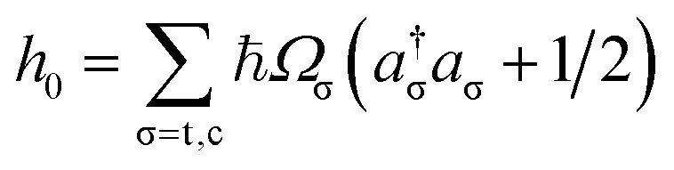
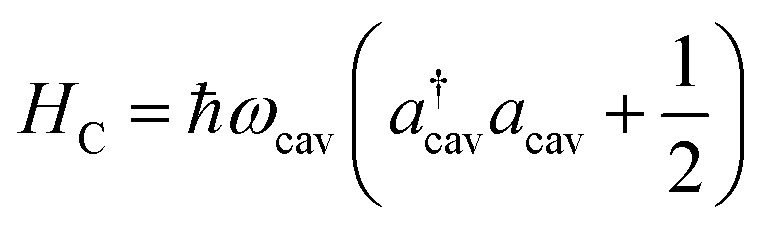
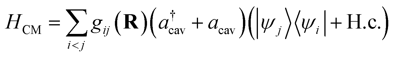
The Hamiltonian of a molecule placed in an optical cavity. consists of the molecular Hamiltonian HM, the cavity photon Hamiltonian HC, and the cavity–matter interaction HCM, and the classical light–matter interaction HLM(t)| | | H = HM + HC + HCM + HLM(t). | (1) |
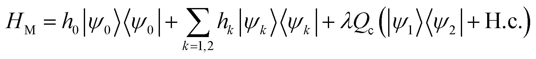
The linear-vibronic coupling model of pyrazine developed in ref. 34 includes three electronic states and two vibrational modes that strongly couple to the electronic motion. It has been widely used to study the nonadiabatic dynamics of pyrazine through the CI.35,36 In the diabatic representation, the molecular Hamiltonian reads
| |  | (2) |
with
hk =
h0 +
Ek +
κkQt,

and H.c. stands for the Hermitian conjugate. Here
Ωσ and
Qσ denote, respectively, the frequency and dimensionless coordinate of the σ-th vibrational mode (σ = c for the coupling mode and σ = t for the tuning mode), {|
ψk〉} are the diabatic electronic states,
Ek is the vertical excitation energy at the Frank–Condon point for
k-th electronic state,
κk are the intra-state electron-vibrational coupling constant, and
λ denotes the interstate coupling strength. The parameters in
HM are
35ħωc = 118 meV,
ħωt = 74 meV,
E1 = 3.94 eV,
E2 = 4.84 eV,
κ1 = −105 meV,
κ2 = 149 meV.
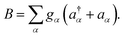
The cavity Hamiltonian is given by
| |  | (3) |
where
ωcav is the resonance frequency of the single cavity mode and
acav (
a†cav) is the annihilation (creation) operator of the cavity photon. The cavity–molecule interaction is described by the electric-dipole coupling
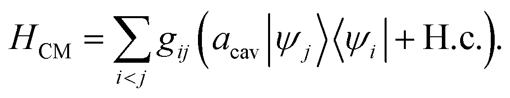
| | 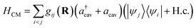 | (4) |
where
g is the coupling strength and
R denotes nuclear coordinates. Invoking the rotating-wave approximation (RWA) and the Condon approximation for the transition dipole in the diabatic representation (
i.e., neglecting the nuclear dependence of the transition dipole moment among diabatic states), the cavity–molecule interaction becomes
| |  | (5) |
The classical light–matter interaction HLM(t) contains the interaction between the molecule and light pulses used in the TAS optical measurement – an actinic and a probe pulse (see the ESI†).
2.2 Nonadiabatic polariton dynamics
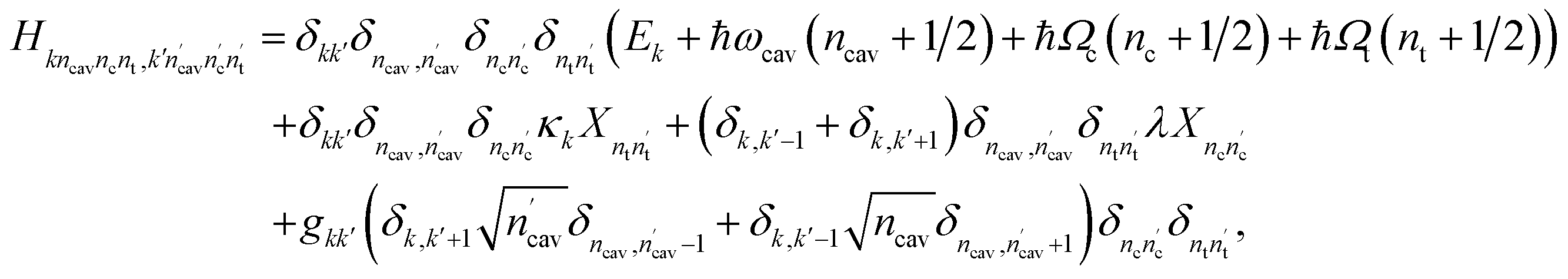
The nonadiabatic dynamics of pyrazine in the optical cavities is simulated numerically exactly by solving the time-dependent Schrödinger equation in a complete basis set of the full polaritonic space – the direct product of the electronic space, vibrational space for the coupling and tuning modes, and the cavity photon space. More precisely, a polaritonic basis function is constructed as a direct product of the diabatic electronic state |ψk〉, number state of the cavity photon mode |ncav〉, the number state of the coupling vibrational mode |nc〉 and the number state of the tuning vibrational mode |nt〉, i.e.,| | | |kncavncnt〉 = |ψk〉 ⊗ |ncav〉 ⊗ |nc〉 ⊗ |nt〉 | (6) |
In this basis set, the matrix elements of H in the absence of classical laser pulses is given by| |  | (7) |
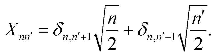
Here X is the position matrix elements in the number state basis 
2.3 The polaritonic potential energy surfaces
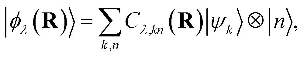
Multiple theoretical frameworks have been developed for the dynamics in optical cavities.1,37 The nonadiabatic polaritonic dynamics presented here is most conveniently understood in the PPESs. The PPESs are analogous to the APESs with the polaritonic states replacing the adiabatic electronic states. Under the separation of timescales of the electron-photonic and the nuclear motion (Born–Oppenheimer-like approximation), the polaritonic states are defined as the eigenstates of the polaritonic Hamiltonian Hp(r,q;R) = Hel(r;R) + HC(q) + HCM(q,r;R) which depends parametrically on the nuclear configuration| | | Hp(r,q;R)|Φn(R)〉 = En(R)|Φn(R)〉 | (8) |
where r, q, R denotes the electronic, photonic, and nuclear coordinates, respectively. Here Hel = HM − Tn is the electronic (or Born–Oppenheimer) Hamiltonian consisting of the electronic kinetic energy operator, electron–electron interaction, electron–nucleus interaction, and nuclei–nuclei interaction, i.e., full molecular Hamiltonian without the nuclear kinetic energy. The polaritonic states reside in the composite space of the electronic and photonic subspaces, and can be expanded in the product basis set of the electronic states and photon Fock states, i.e.,  where the expansion coefficients can be obtained by solving eqn (8).
Alternatively, one can define a potential energy surface in the joint photon-nuclear space
| | | Hp(r;q,R)|Φn(q,R)〉 = En(q,R)|Φn(q,R)〉. | (9) |
This can be useful for numerical simulations of polaritonic dynamics,
38 especially in the ultrastrong coupling regime where rotating wave approximation does not apply.
2.4 Effects of the external environment
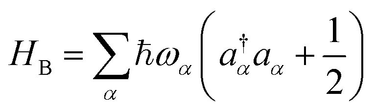
Polaritonic systems inevitably interact with external environments, which can induce significant changes in their dynamics through energy relaxation and decoherence. The environment for the cavity photon are the photonic modes outside the cavity accessible via the imperfect reflections of the cavity mirrors. This interaction leads to a finite lifetime of the cavity photon mode. For femtosecond dynamics we can neglect the slower decay of the cavity mode. However, the environment for the molecular motion (e.g., solvent) may have a large influence on the nonadiabatic polaritonic dynamics through ultrafast electronic decoherence processes.39–41
We introduce an external environment  consisting of a collection of harmonic oscillators with frequencies {ωα} described by the creation a†α and annihilation operators aα. The molecule-bath coupling describing the decoherence effects between two electronic states |ψi〉 and |ψj〉 is given by
| |  | (10) |
where we have introduced the system and bath operator
S = |
ψj〉〈
ψj| − |
ψi〉〈
ψi| and
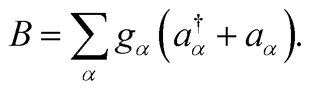
The influence of the environment on the molecule is encoded in the spectral density
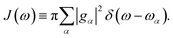
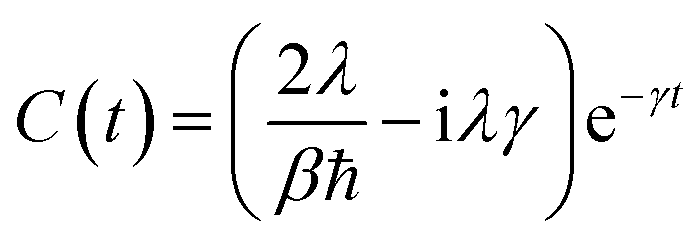
We assume an Ohmic spectral density with a Lorentz–Drude cutoff
| | | J(ω) = 2λωγ/(ω2 + γ2) | (11) |
where
γ is the cutoff frequency and
λ is the reorganization energy characterizing the system–bath coupling strength.
To account for the non-Markovian effects of the environment, we use the non-perturbative hierarchical equation of motion method.42 In this method, the reduced dynamics of the primary polaritonic system is described by a set of coupled differential equations (ℏ = 1; see the ESI† for a summary of this technique)
| |  | (12) |
where

are superoperators defined in the Liouville space, and {
ρn,
n = 0, 1,…} are the auxiliary density operators with the first element corresponding to the reduced density matrix of the system
ρS(
t) =
ρ0(
t). Here
C(
t) = 〈
BI(
t)
B〉 is the environment time-correlation function where
BI(
t) = e
+iHBtB![[thin space (1/6-em)]](https://www.rsc.org/images/entities/char_2009.gif)
e
−iHBt is the bath operator
B in the interaction picture of
HB. For environments at thermal equilibrium with inverse temperature
β = 1/(
kBT), it can be evaluated from the spectral density (details can be found in the ESI
†)
| |  | (13) |
In the high-temperature limit
βℏγ < 1, coth(
βℏω/2) ≈ 2/(
βℏω) and the correlation function becomes
| | 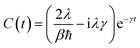 | (14) |
2.5 The transient absorption signal
The polaritonic nonadiabatic dynamics typically occurs in the femtosecond timescale. Therefore, ultrafast time-resolved spectroscopy such as TAS can unveil the dynamic features induced by the strong light–matter coupling in optical cavities. TAS is a pump–probe technique capable of providing useful information on the population changes of excited molecules.43 The molecule is first excited to an electronically excited state by an ultrashort pump pulse, and after a certain delay time T, a probe pulse interrogates the molecule by measuring the state-occupation changes. The theory for TAS for molecules in cavities and the computational details are given in the ESI.†
3 Results and discussion
3.1 Polaritonic dynamics
Because the pyrazine model contains three electronic states, there are several ways the molecule can be coupled to the cavity. In the following we consider two scenarios that lead to distinct polaritonic nonadiabatic dynamics.
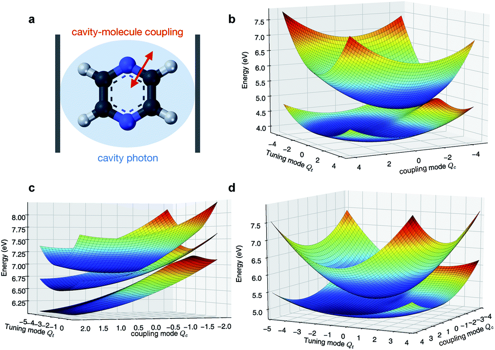
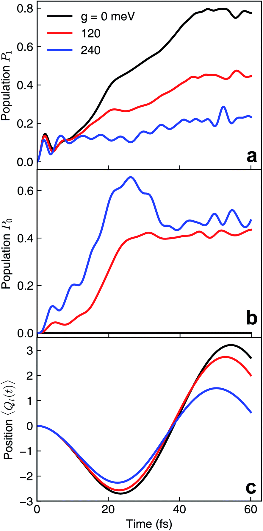
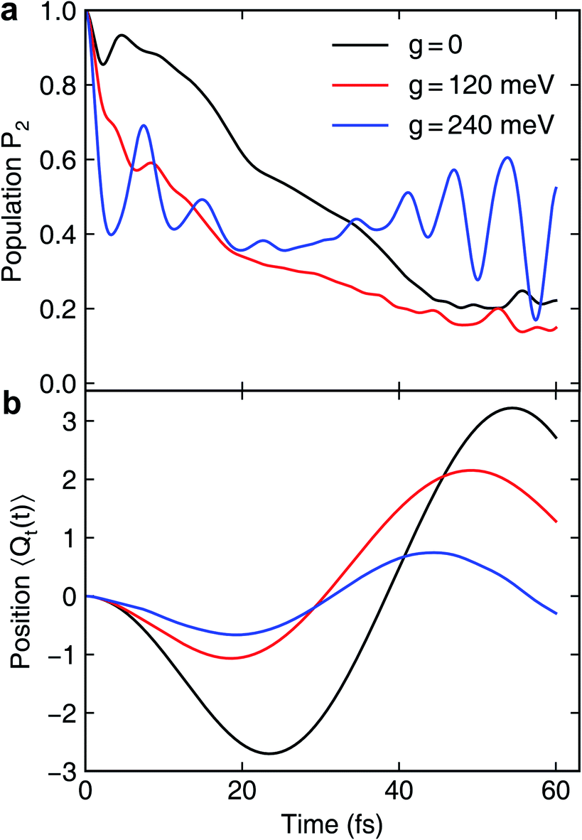
We first assume that the cavity photon mode couples to the |ψ0〉 ↔ |ψ1〉 transition. The cavity resonant frequency ωcav = 4.3 eV is close to the transition energy |ψ0〉 → |ψ1/2〉 at the CI point. The polaritonic surfaces are shown in Fig. 1c for the cavity–molecule coupling strength g01 = 124 meV. The electronic state population dynamics at different cavity–molecule coupling strength is shown in Fig. 2. The molecule is prepared at electronic state |ψ2〉. The population dynamics of states |ψ1〉 and |ψ0〉 are shown in Fig. 2a and b, respectively, and the average value of the tuning mode is shown in Fig. 2c. Without the cavity, the nuclear wavepacket traverses through the CI and, due to the strong electron-nuclear coupling, the electronic excitation relaxes to |ψ1〉 within 30 fs, see also Fig. 1b for the APESs of the model pyrazine without cavity–molecule coupling. The ground electronic state |ψ0〉 is not populated during the dynamics as it is decoupled from the two excited electronic states.
 |
| | Fig. 1 Born–Oppenheimer (adiabatic) and polaritonic potential energy surfaces of the pyrazine model coupled to the cavity photon mode. The adiabatic and polaritonic surfaces are computed by diagonalizing the electronic and polaritonic Hamiltonian, respectively, scanning the nuclear configurations. (a) Schematic of the pyarzine molecule placed inside an optical cavity. (b) Adiabatic potential energy surfaces of the first and second excited states. (c) Polaritonic surfaces (relevant to the dynamics) when the cavity mode couples to the |ψ0〉 ↔ |ψ1〉 transition. Here ωcav = 4.3 eV and g01 = 124 meV. (d) Same as (c) but for the cavity photon mode coupling to the |ψ1〉 ↔ |ψ2〉 transition. Here ωcav = 0.62 eV and g12 = 124 meV. | |
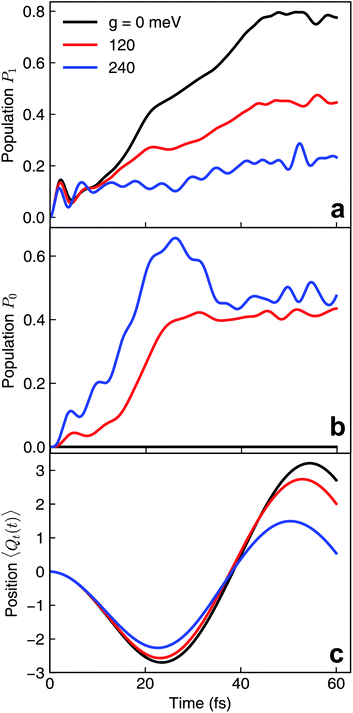 |
| | Fig. 2 Nonadiabatic polaritonic dynamics for the pyrazine model when a cavity mode with frequency ωcav = 4.3 eV couples to the |ψ0〉 ↔ |ψ1〉 transition at different cavity–molecule coupling strength. (a and b) Population dynamics of electronic states (a) |ψ1〉 and (b) |ψ0〉. (c) Expectation value of the position of the tuning mode 〈Ψ(t)|Qt|Ψ(t)〉 where |Ψ(t)〉 is the full polaritonic wavefunction. | |
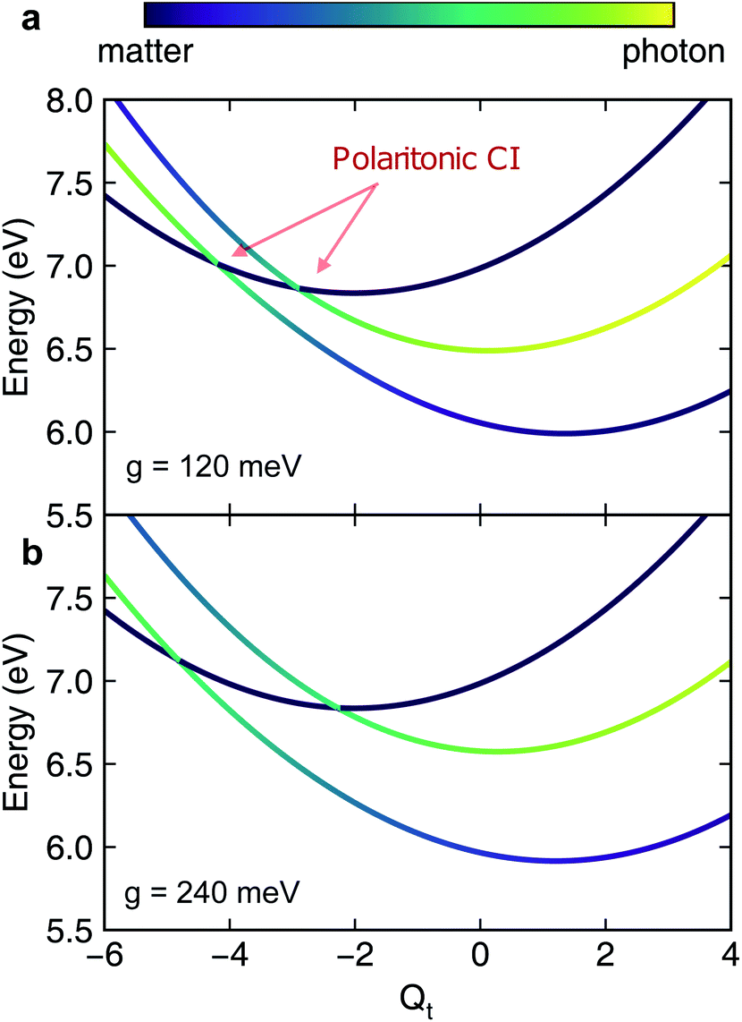
When the cavity photon mode is coupled to the molecular transition |ψ0〉 ↔ |ψ1〉, the electronic excitation directly relaxes back to the ground state as shown in Fig. 2b, in contrast to the nonadiabatic dynamics of the bare molecule. This implies that the strong light–matter coupling creates a channel for such relaxation process. The relaxation to the ground state is accompanied by the decrease of populations in the first electronic state with the overall relaxation dynamics accelerated by the strong coupling. The significant cavity-induced changes in the nonadiabatic dynamics can be understood from the shape of the PPESs. As shown in Fig. 3, the cavity–molecule coupling creates two new CIs in the PPESs. Distinct from the bare CI in the APES, these CIs are between a purely electronic state |ψ2〉 and another polaritonic state with significant hybridization of matter and photon, as reflected in the color scheme which encodes the photon component in polaritonic states. More precisely, it corresponds to the expected photon number Nph = 〈Φ(R)|a†cavacav|Φ(R)〉with the polaritonic state |Φ(R)〉, which is a superposition of states |ψ0〉|1cav〉 and |ψ1〉|0cav〉. The polaritonic CIs play similar roles in the nonadiabatic polaritonic dynamics as CIs play in the nonadiabatic dynamics of pristine molecules. While CIs in APESs induce transitions between electronic states, polaritonic CIs induce transitions in the polaritonic surfaces. The nuclear wavepacket first traverses through one of the polaritonic CIs that is closer to the Franck–Condon point R ≡ (Qc, Qt) = (0, 0), part of the nuclear wavepacket relaxes to the third PPES (the ground surface is not shown in Fig. 3). Because the polaritonic states of this PPES consist of the contribution from |ψ0〉|1cav〉, the electronic ground state gains population during the course of dynamics. This picture is further confirmed by the expectation value of the position operator of the tuning mode. As the cavity–molecule coupling strength increases, the polaritonic CI is pushed further away from the pristine CI, thus explaining the increase of the average position of the nuclear wavepacket at t ∼ 25 fs.
 |
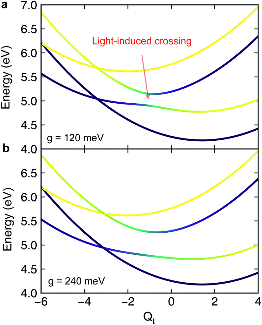
| | Fig. 3 Slices of the polaritonic potential energy surfaces along the tuning mode when the cavity mode couples to |ψ0〉 ↔ |ψ1〉 at different light–matter coupling strength (a) g ≡ g01 = 120 meV and (b) g = 240 meV. Other parameters are Qc = 0, ωcav = 4.3 eV. The pristine conical intersection (CI) in the adiabatic potential energy surfaces splits into a pair of novel polaritonic CIs in the polaritonic surfaces upon coupling to the cavity photon mode. | |
As the polaritonic CI is closer to the Franck–Condon point, the geometric phase effect is clearly observed in Fig. 4, which compares the nuclear probability density at t = 32 fs in electronic state |S1〉 between the bare dynamics and the polaritonic dynamics (g = 240 meV). The nuclear probability density is obtained by tracing over the electronic and photonic degrees of freedom in the total wavefunction projected on the electronic subspace  i.e.,
i.e.,  The geometric phase effect is clearly seen in the vanishing of the probability along the Qc = 0 line in the polaritonic dynamics (Fig. 4b). The main difference is that ρn(R) is less spread over the configuration space than the bare dynamics, meaning that less excitation energy flows into the vibrational modes. This is expected because part of the energy is contained in the cavity photon mode.
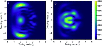 |
| | Fig. 4 Comparison of the nuclear probability density at t = 32 fs between (a) the bare dynamics and (b) the polaritonic dynamics at g = 240 meV. The geometric phase effect is clearly seen in the vanishing of probability along the Qc = 0 line. | |
It is interesting to compare the novel polaritonic CI to the light-induced CI identified previously.1,31 In the latter case, the conical intersection is between two product states between the molecule and the cavity at configurations where the cavity–molecule interaction (transition dipole moments) vanishes. In other words, |g〉 ⊗ |1cav〉 and |e〉 ⊗ |0cav〉 are degenerate when μeg·e = 0, where μeg is the transition dipole between states |e〉 and |g〉 and e is the polarization vector of the cavity photon mode, and the transition energy is resonant with the cavity photon energy. When one of the nuclear coordinates is a rotation, this CI can be realized at the angle where the transition dipole is orthogonal to the polarization of the cavity photon. It does not require a pristine CI in the molecule and the CI geometry is not affected by the light–matter coupling strength. In contrast, the novel pair of polaritonic CIs are between two hybrid polaritonic states. This emerges when the molecule itself contains a CI in the APESs and when the cavity mode couples to the transition between one of the APESs forming the bare CI and a third electronic state. Moreover, the polaritonic CIs geometry can be tuned by the strength of light–matter coupling strength. As the cavity–molecule coupling is increased to gcav = 240 meV, the positions of the two polaritonic CIs are further apart. This change of the location of polaritonic CI can also be seen in the average position of the tuning mode, see Fig. 2c. Population relaxation to the ground electronic state is further increased.
We now turn to a different scenario where the cavity mode couples to the transition |ψ1〉 ↔ |ψ2〉 transition. The PPESs are shown in Fig. 1d for ωcav = 0.62 eV (slightly lower than the transition frequency at the Frank–Condon point) and g12 = 120 meV. In this case, the ground electronic state is not playing any role in the dynamics as it is decoupled from the other electronic states. Upon turning on the light–matter interaction, we first observe a much faster electronic relaxation as shown in Fig. 5a. The relaxation time reduces from 30 fs without the cavity to ∼15 fs at g12 = 120 meV. Interestingly, as can be seen from the average position of the tuning mode in Fig. 5b, the nuclear wavepacket does not even reach the pristine conical intersection. Similar to the previous analysis, we interpret the nonadiabatic polaritonic dynamics from the shape of PPESs shown in Fig. 6. The main feature of the polaritonic surfaces is the emergence of a light-induced (avoided) crossing. This offers an additional electronic relaxation channel other than the pristine CI. Because the light-induced crossing is much closer to the Franck–Condon point in this case, the relaxation happens mainly through this channel and consequently, the relaxation happens much faster. As the coupling strength is enhanced, the relaxation rate is further increased.
 |
| | Fig. 5 Nonadiabatic polaritonic dynamics for the pyrazine model when the cavity mode couples to the |ψ1〉 ↔ |ψ2〉 transition at different cavity–molecule coupling strength. (a) Population dynamics of electronic state |ψ2〉. (b) Expectation value of the position of the tuning mode. | |
 |
| | Fig. 6 Same as Fig. 3 but with the cavity photon mode coupling to the transition |ψ1〉 ↔ |ψ2〉 and g ≡ g12. The characteristic feature of the polaritonic surfaces is the light-induced crossing providing an additional channel for electronic relaxation. | |
Interestingly, this light-induced avoided crossing is always associated with a light-induced CI. This is because one can always rotate the molecule such that the transition dipole at the configuration R*, where the electronic transition is in resonance with the cavity photon energy, is orthogonal to the electric field polarization. Since we can always find such molecular geometry R* in an avoided crossing, the light-induced CI is guaranteed to exist.
For case II, the counterrotating terms that are neglected in the rotating-wave approximation [eqn (5)] may become important as the coupling strength becomes comparable to the cavity resonance (so-called ultrastrong coupling). To investigate the influences of counterrotating terms, we simulate the polaritonic dynamics employing the full interaction as in eqn (4). As shown in Fig. S2† where the dynamics with and without the RWA are contrasted, when g = 120 meV [Fig. S2(a and b)†], there is only minor changes in the polaritonic dynamics without invoking the RWA. For g = 240 meV [Fig. S2(c and d)†], the counterrotating terms start to play a role in the long-time dynamics t > 40 fs, but the intial relaxation dynamics (t ∈ [0, 40] fs) remains almost the same.
3.2 Environmental effects
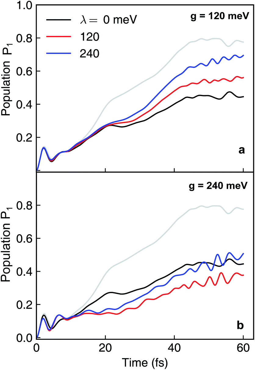
We now explore the external environmental effects on the nonadiabatic polaritonic dynamics. In our simulations, the environment is coupled to the same pair of electronic states that are coupled to the cavity photon mode. We note some common features that apply to all cases. First, even when the reorganization energy is twice the cavity–molecule coupling strength, i.e., λ/g = 2, an appreciable difference between the bare dynamics and the polaritonic dynamics can still be observed implying that the cavity-controlled photochemistry can be robust to electronic decoherence. Further, while the environment is expected to destroy the phase coherence in a superposition of electronic states, it does not happen instantaneously and there is a characteristic timescale where the system dynamics is almost not influenced by the presence of environment, reminiscent of the quantum Zeno effects. This timescale can be estimated by the decoherence time for the environment to reduce an equal superposition of a two-level system to a mixed state44,45 For λ = 240 meV, T = 300 K, τc ≈ 9 fs. This is consistent with the time where environmental effects becomes noticeable in the polaritonic dynamics.
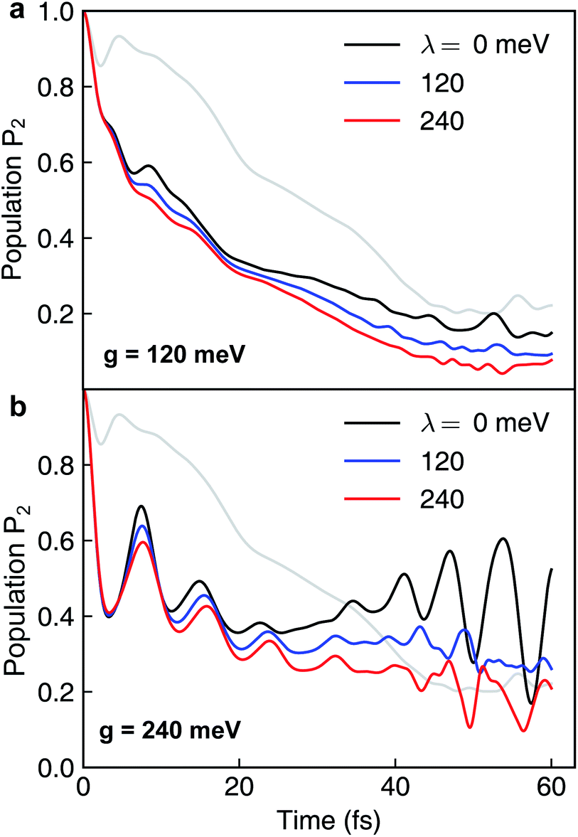
Because the formation of cavity polaritons relies on the coherence between electronic states, the environment is expected to diminish the cavity control. This is indeed seen in the population dynamics of electronic state |ψ2〉 in case I when g = 120 meV (Fig. 7a). When the cavity–molecule coupling is stronger, this deleterious effect becomes less significant (Fig. 7b). Another effect of the environment is reflected in case II where the coherent population transfer between electronics states |ψ2〉 and |ψ1〉 at g = 240 meV during the time periods 0–20 fs and 40–60 fs is reduced (Fig. 8b). The polaritonic dynamics at g = 120 meV in case II is almost immune to the external environment (Fig. 8a), the dissipative polaritonic dynamics for all system–bath coupling strengths λ/g = 0, 1, 2 shows the same timescale ∼20 fs for the electronic relaxation in comparison to 40 fs in the bare molecule case. This implies that the relaxation channel provided by the light-induced crossing is robust to the environment.
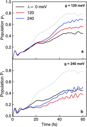 |
| | Fig. 7 Dissipative nonadiabatic polaritonic dynamics simulated by the hierarchical equations of motion when both the cavity mode and the external environment couples to the transition |ψ0〉 ↔ |ψ1〉 at system–bath coupling strength λ = 0, 120, 240 meV. The grey line corresponds to the nonadiabatic dynamics of bare molecules without cavity. The cavity parameters are ωcav = 4.3 eV, the cavity–molecule couplings are (a) g = 120 meV and (b) g = 240 meV. | |
 |
| | Fig. 8 Same as Fig. 7 but for both the cavity mode and the external environment coupled to the transition |ψ1〉 ↔ |ψ2〉. The cavity parameters are ωcav = 0.62 eV, the cavity–molecule couplings are (a) g = 120 meV and (b) g = 240 meV. | |
3.3 The transient absorption spectrum
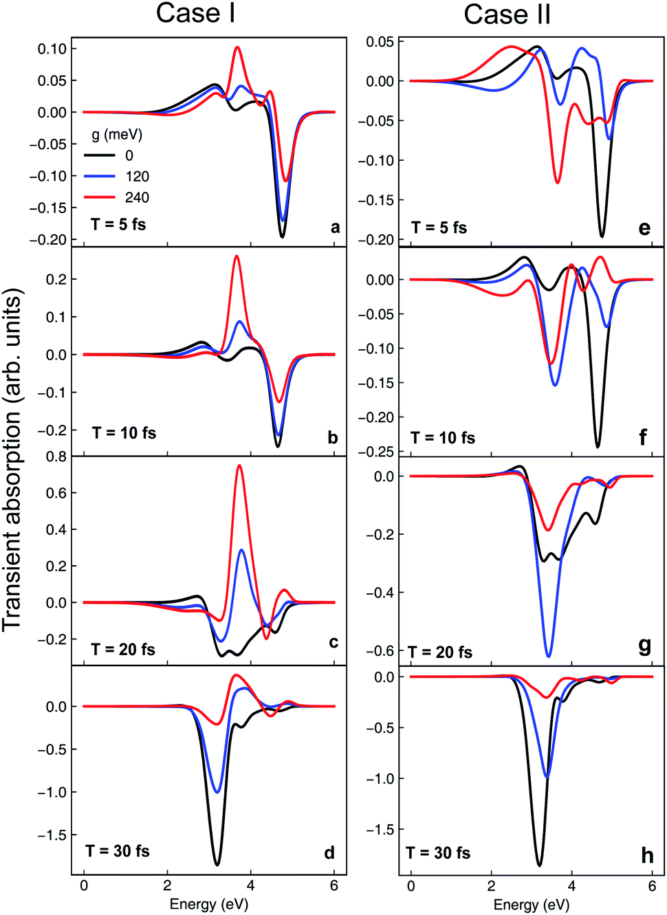
The cavity-induced changes in the nonadiabatic dynamics can be clearly observed in TAS. Computational details of the TAS can be found in the ESI.† For pyrazine, the transition dipole between states |ψ0〉 and |ψ2〉 is much larger than the transition between |ψ0〉 and |ψ1〉. As shown in Fig. 9a–d, the main feature of the TAS for the bare nonadiabatic dynamics (i.e., without the cavity) is a negative peak (stimulated emission) at ∼3.2 eV growing during the course of dynamics accompanied by the diminishing of the stimulated emission peak at 4.8 eV. This arises from the stimulated emission from electronic state |ψ1〉 to the ground state, and the increasing intensity corresponds to the population relaxation dynamics. In contrast, when the molecule is strongly coupled to the cavity as in case I, we observe a positive peak centered around 3.8 eV in the TAS. As a positive signal represents absorption of energy from the probe laser pulse, this feature is a signature of population relaxation to the ground electronic state. Further, when g01 = 240 meV (Fig. 9f), the absorption signal at t = 20 fs is much stronger than g01 = 120 meV, indicating that the relaxation to the ground state is faster with stronger coupling, consistent with the dynamics. The TAS for case II is shown in Fig. 9e–h. The stimulated emission |ψ1〉 → |ψ0〉 peak emerges as early as T = 5 fs (Fig. 9e), much earlier than the bare nonadiabatic dynamics, indicating that the relaxation is much faster when the molecule is under strong coupling, consistent with the picture of cavity-induced crossings.
 |
| | Fig. 9 Transient absorption spectra of the model pyrazine under strong coupling for case I (a–d) and II (e–h) at different cavity–molecule coupling strength. Here T is the time delay between the pump and probe pulses. | |
4 Conclusions
To summarize, we have investigated how optical cavities can be used to manipulate the nonadiabtic molecular dynamics through a conical intersection. In contrast to a recent study46 where the cavity is tuned to be in resonance with the Frank–Condon transition thus altering the initial photoexcitation, we investigated schemes where the molecules have to undergo a structural change to be in resonance with the cavity mode. By considering three electronic state model of pyrazine, we unveil that optical cavities, when coupled to the transition between one of the states comprising the CI and a third state, can split the pristine conical intersection in the APESs into two novel polaritonic conical intersections in the PPESs. By tuning the cavity–molecule coupling strength, it is possible to vary the configurations of the polaritonic conical intersection pairs. This may serve as a novel control scheme to preserve electronic coherence in molecules because electronic coherence depends sensitively on the location of the CI.45,47,48 In the other case where the cavity photon couples to the two electronic states forming the CI, we found light-induced avoided crossings in the polaritonic potential energy surfaces, which provide additional relaxation channel for electronic excitation, and thus can accelerate the nonradiative relaxation dynamics. This light-induced crossing has also been suggested to manipulate the photoisomerization of azobenzene in a recent trajectory-surface hopping study.31 While the trajectory-surface hopping method cannot take electronic coherence as well as geometric phase into account properly, our simulations do not suffer from such limitations.
We further explored the environmental effects on the polaritonic dynamics and demonstrated that even when the reorganization energy is larger than the cavity–molecule coupling, the optical cavities can still be employed to manipulate the photodynamics of molecules. Moreover, we showed that the TAS can be a useful spectroscopic technique to monitor the polaritonic dynamics. These results provide novel schemes to control the non-adiabatic dynamics with strong light–matter coupling, enriching the toolbox to use optical cavities to alter molecular properties and dynamics. Considering the rapid developments in nanophotonics,49,50 we expect that polaritonic systems can be experimentally investigated in the forseeable future. The strong coupling can be also achieved through the collective interaction between many molecules and a single cavity mode, extending the proposed control schemes to photochemistry with many molecules will be investigated in the future.
Conflicts of interest
There are no conflicts to declare.
Acknowledgements
This work was supported by the National Science Foundation Grant CHE-1663822.
Notes and references
- M. Kowalewski, K. Bennett and S. Mukamel, J. Chem. Phys., 2016, 144, 054309 CrossRef PubMed.
- K. Bennett, M. Kowalewski and S. Mukamel, Faraday Discuss., 2016, 194, 259–282 RSC.
- T. W. Ebbesen, Acc. Chem. Res., 2016, 49, 2403–2412 CrossRef CAS PubMed.
- X. Zhong, T. Chervy, S. Wang, J. George, A. Thomas, J. A. Hutchison, E. Devaux, C. Genet and T. W. Ebbesen, Angew. Chem., 2016, 128, 6310–6314 CrossRef.
- X. Zhong, T. Chervy, L. Zhang, A. Thomas, J. George, C. Genet, J. A. Hutchison and T. W. Ebbesen, Angew. Chem., Int. Ed., 2017, 56, 9034–9038 CrossRef CAS PubMed.
- J. George, A. Shalabney, J. A. Hutchison, C. Genet and T. W. Ebbesen, J. Phys. Chem. Lett., 2015, 6, 1027–1031 CrossRef CAS PubMed.
- A. Shalabney, J. George, J. Hutchison, G. Pupillo, C. Genet and T. W. Ebbesen, Nat. Commun., 2015, 6, 5981 CrossRef CAS PubMed.
- F. Benz, M. K. Schmidt, A. Dreismann, R. Chikkaraddy, Y. Zhang, A. Demetriadou, C. Carnegie, H. Ohadi, B. de Nijs, R. Esteban, J. Aizpurua and J. J. Baumberg, Science, 2016, 354, 726–729 CrossRef CAS PubMed.
- A. Thomas, L. Lethuillier-Karl, K. Nagarajan, R. M. A. Vergauwe, J. George, T. Chervy, A. Shalabney, E. Devaux, C. Genet, J. Moran and T. W. Ebbesen, Science, 2019, 363, 615–619 CrossRef CAS PubMed.
- A. Shalabney, J. George, H. Hiura, J. A. Hutchison, C. Genet, P. Hellwig and T. W. Ebbesen, Angew. Chem., Int. Ed., 2015, 54, 7971–7975 CrossRef CAS PubMed.
- C. Schäfer, M. Ruggenthaler, H. Appel and A. Rubio, Proc. Natl. Acad. Sci. U. S. A., 2019, 116, 4883–4892 CrossRef PubMed.
- J. Galego, F. J. Garcia-Vidal and J. Feist, Phys. Rev. X, 2015, 5, 041022 Search PubMed.
- J. Flick and P. Narang, Phys. Rev. Lett., 2018, 121, 113002 CrossRef CAS PubMed.
- K. E. Dorfman and S. Mukamel, Proc. Natl. Acad. Sci. U. S. A., 2018, 115, 1451–1456 CrossRef CAS PubMed.
- F. Herrera and F. C. Spano, Phys. Rev. Lett., 2016, 116, 238301 CrossRef PubMed.
- D. M. Coles, N. Somaschi, P. Michetti, C. Clark, P. G. Lagoudakis, P. G. Savvidis and D. G. Lidzey, Nat. Mater., 2014, 13, 712–719 CrossRef CAS PubMed.
- A. Frisk Kockum, A. Miranowicz, S. De Liberato, S. Savasta and F. Nori, Nat. Rev. Phys., 2019, 1, 19–40 CrossRef.
- P. Vasa and C. Lienau, ACS Photonics, 2018, 5, 2–23 CrossRef CAS.
- M. Hertzog, M. Wang, J. Mony and K. Börjesson, Chem. Soc. Rev., 2019, 48, 937–961 RSC.
- J. A. Hutchison, T. Schwartz, C. Genet, E. Devaux and T. W. Ebbesen, Angew. Chem., Int. Ed., 2012, 51, 1592–1596 CrossRef CAS PubMed.
- J. Flick, M. Ruggenthaler, H. Appel and A. Rubio, Proc. Natl. Acad. Sci. U. S. A., 2017, 114, 3026–3034 CrossRef CAS PubMed.
- T. Schwartz, J. A. Hutchison, J. Léonard, C. Genet, S. Haacke and T. W. Ebbesen, ChemPhysChem, 2013, 14, 125–131 CrossRef CAS PubMed.
- F. Herrera and F. C. Spano, ACS Photonics, 2018, 5, 65–79 CrossRef CAS.
- L. A. Martínez-Martínez, M. Du, R. F. Ribeiro, S. Kéna-Cohen and J. Yuen-Zhou, J. Phys. Chem. Lett., 2018, 9, 1951–1957 CrossRef PubMed.
- D. Sanvitto and S. Kéna-Cohen, Nat. Mater., 2016, 15, 1061–1073 CrossRef CAS PubMed.
- A. Mandal and P. Huo, J. Phys. Chem. Lett., 2019, 10, 5519–5529 CrossRef CAS PubMed.
- M. Du, R. F. Ribeiro and J. Yuen-Zhou, Chem, 2019, 5, 1167–1181 CAS.
-
J. B. Pérez-Sánchez and J. Yuen-Zhou, arXiv: 1909.13024, 2019.
- O. Vendrell, Phys. Rev. Lett., 2018, 121, 253001 CrossRef CAS PubMed.
- T. Szidarovszky, G. J. Halász, A. G. Császár, L. S. Cederbaum and Á. Vibók, J. Phys. Chem. Lett., 2018, 9, 6215–6223 CrossRef CAS PubMed.
- J. Fregoni, G. Granucci, E. Coccia, M. Persico and S. Corni, Nat. Commun., 2018, 9, 4688 CrossRef CAS PubMed.
- Y. Tanimura, J. Phys. Soc. Jpn., 2006, 75, 082001 CrossRef.
- Y. Tanimura and R. Kubo, J. Phys. Soc. Jpn., 1989, 58, 101–114 CrossRef.
- C. Woywod, W. Domcke, A. L. Sobolewski and H.-J. Werner, J. Chem. Phys., 1994, 100, 1400–1413 CrossRef CAS.
- L. Chen, M. F. Gelin, V. Y. Chernyak, W. Domcke and Y. Zhao, Faraday Discuss., 2016, 194, 61–80 RSC.
- M. Sala and D. Egorova, Chem. Phys., 2016, 481, 206–217 CrossRef CAS.
- J. Flick, H. Appel, M. Ruggenthaler and A. Rubio, J. Chem. Theory Comput., 2017, 13, 1616–1625 CrossRef CAS PubMed.
- K. Bennett, M. Kowalewski and S. Mukamel, J. Chem. Theory Comput., 2016, 12, 740–752 CrossRef CAS PubMed.
-
H.-P. Breuer and F. Petruccione, The Theory of Open Quantum Systems, Oxford University Press, 2002 Search PubMed.
- B. Gu and I. Franco, J. Chem. Phys., 2019, 151, 014109 CrossRef PubMed.
- W. Hu, B. Gu and I. Franco, J. Chem. Phys., 2018, 148, 134304 CrossRef PubMed.
- Y. Tanimura and S. Mukamel, J. Chem. Phys., 1993, 99, 9496–9511 CrossRef CAS.
- Z. Wang, W. Wu, G. Cui and J. Wang, New J. Phys., 2018, 20, 033034 CrossRef.
- O. V. Prezhdo and P. J. Rossky, Phys. Rev. Lett., 1998, 81, 5294–5297 CrossRef CAS.
- B. Gu and I. Franco, J. Phys. Chem. Lett., 2018, 9, 773–778 CrossRef CAS PubMed.
- I. S. Ulusoy, J. A. Gomez and O. Vendrell, J. Phys. Chem. A, 2019, 123, 8832–8844 CrossRef CAS PubMed.
- C. Arnold, O. Vendrell, R. Welsch and R. Santra, Phys. Rev. Lett., 2018, 120, 123001 CrossRef CAS PubMed.
- B. Gu and I. Franco, J. Phys. Chem. Lett., 2017, 8, 4289–4294 CrossRef CAS PubMed.
- P. Forn-Díaz, L. Lamata, E. Rico, J. Kono and E. Solano, Rev. Mod. Phys., 2019, 91, 025005 CrossRef.
- R. Chikkaraddy, B. de Nijs, F. Benz, S. J. Barrow, O. A. Scherman, E. Rosta, A. Demetriadou, P. Fox, O. Hess and J. J. Baumberg, Nature, 2016, 535, 127–130 CrossRef CAS PubMed.
Footnote |
| † Electronic supplementary information (ESI) available: (i) Theory and computational protocol of transient absorption spectroscopy for polaritonic chemistry, and (ii) the hierarchical equations of motion method, and relation between spectral density and environment correlation function [eqn (13)]. See DOI: 10.1039/c9sc04992d |
|
| This journal is © The Royal Society of Chemistry 2020 |
Click here to see how this site uses Cookies. View our privacy policy here. 
 Open Access Article
 This Open Access Article is licensed under a Creative Commons Attribution-Non Commercial 3.0 Unported Licence
 *a and
Shaul
Mukamel
*a and
Shaul
Mukamel
 and H.c. stands for the Hermitian conjugate. Here Ωσ and Qσ denote, respectively, the frequency and dimensionless coordinate of the σ-th vibrational mode (σ = c for the coupling mode and σ = t for the tuning mode), {|ψk〉} are the diabatic electronic states, Ek is the vertical excitation energy at the Frank–Condon point for k-th electronic state, κk are the intra-state electron-vibrational coupling constant, and λ denotes the interstate coupling strength. The parameters in HM are35ħωc = 118 meV, ħωt = 74 meV, E1 = 3.94 eV, E2 = 4.84 eV, κ1 = −105 meV, κ2 = 149 meV.
 where the expansion coefficients can be obtained by solving eqn (8).
 consisting of a collection of harmonic oscillators with frequencies {ωα} described by the creation a†α and annihilation operators aα. The molecule-bath coupling describing the decoherence effects between two electronic states |ψi〉 and |ψj〉 is given by
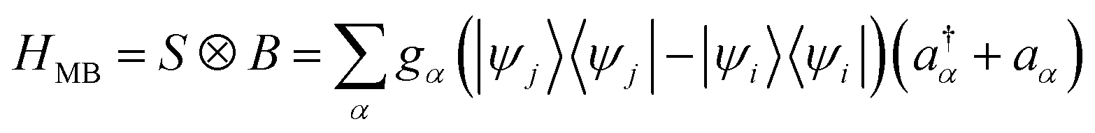
 The influence of the environment on the molecule is encoded in the spectral density
 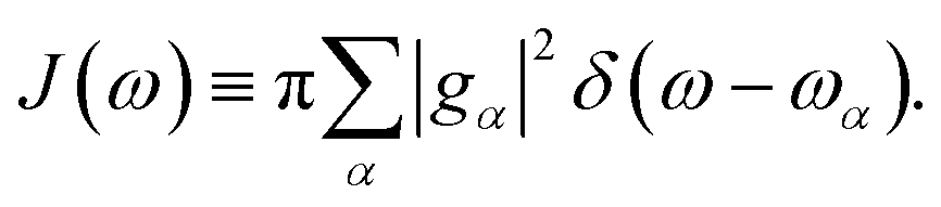 We assume an Ohmic spectral density with a Lorentz–Drude cutoff
 are superoperators defined in the Liouville space, and {ρn, n = 0, 1,…} are the auxiliary density operators with the first element corresponding to the reduced density matrix of the system ρS(t) = ρ0(t). Here C(t) = 〈BI(t)B〉 is the environment time-correlation function where BI(t) = e+iHBtB
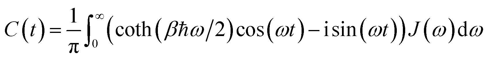
 i.e.,
i.e., 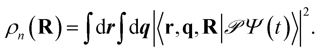 The geometric phase effect is clearly seen in the vanishing of the probability along the Qc = 0 line in the polaritonic dynamics (Fig. 4b). The main difference is that ρn(R) is less spread over the configuration space than the bare dynamics, meaning that less excitation energy flows into the vibrational modes. This is expected because part of the energy is contained in the cavity photon mode.
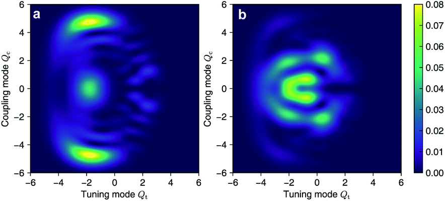
 For λ = 240 meV, T = 300 K, τc ≈ 9 fs. This is consistent with the time where environmental effects becomes noticeable in the polaritonic dynamics.