Large scale relative protein ligand binding affinities using non-equilibrium alchemy

Abstract

Ligand binding affinity calculations based on molecular dynamics (MD) simulations and non-physical (alchemical) thermodynamic cycles have shown great promise for structure-based drug design. However, their broad uptake and impact is held back by the notoriously complex setup of the calculations. Only a few tools other than the free energy perturbation approach by Schrödinger Inc. (referred to as FEP+) currently enable end-to-end application. Here, we present for the first time an approach based on the open-source software pmx that allows to easily set up and run alchemical calculations for diverse sets of small molecules using the GROMACS MD engine. The method relies on theoretically rigorous non-equilibrium thermodynamic integration (TI) foundations, and its flexibility allows calculations with multiple force fields. In this study, results from the Amber and Charmm force fields were combined to yield a consensus outcome performing on par with the commercial FEP+ approach. A large dataset of 482 perturbations from 13 different protein–ligand datasets led to an average unsigned error (AUE) of 3.64 ± 0.14 kJ mol⁻¹, equivalent to Schrödinger's FEP+ AUE of 3.66 ± 0.14 kJ mol⁻¹. For the first time, a setup is presented for overall high precision and high accuracy relative protein–ligand alchemical free energy calculations based on open-source software.

---

Introduction

The lead optimization (LO) stage of drug discovery involves the synthesis of hundreds of lead compound analogs, with the aim to improve multiple properties in parallel. Among these are selectivity against related targets, enhanced metabolic stability, permeability, solubility, reduced side effects, efflux, and plasma protein binding. Thus, LO is a multi-objective optimization problem in which chemists try to identify structure–property relationships that will allow to tune the chemical and biophysical properties of the lead compound. Ligand binding affinity for the primary protein target is central to all LO efforts as it impacts drug efficacy, and thus its dose and selectivity margins versus off-target effects. Computationally-driven guidance to LO requires precision and accuracy, and the predictive power of empirical scoring functions alone is rarely enough at this stage of drug discovery.^1–4 For this data-scarce yet multiparameter problem it remains to be seen if data-driven methods are able to predict new primary target activities. On the other hand, an approach that has shown the required level of performance is alchemical relative binding free energy (RBFE) calculations based on molecular dynamics (MD) simulations.^5–7

Free energy perturbation (FEP)^8,9 and thermodynamic integration (TI)¹⁰ are popular methods used for alchemical RBFE estimation. The application of FEP in alchemical calculations dates back several decades and it typically uses molecular dynamics (MD) or Monte Carlo simulations to compute the free-energy difference between two structurally related ligands, making it ideal for LO.^11–15 Equilibrium FEP is arguably the most common implementation of alchemical calculations and involves many distinct equilibrium MD simulations for all states along a λ coordinate that alchemically modifies the first ligand into the second. It is common to use 12, 15 or more so-called λ intermediates wherein atoms that need to appear, disappear, or mutate between the two ligands are represented by a linear combination of end-state Hamiltonians. During alchemical transformations, van der Waals and sometimes electrostatic interactions are softened to avoid singularities and numerical instabilities.^16–18 Various methods exist to calculate the free energy associated with a change of the λ coordinate, but a requisite for convergence is an overlap in conformational space between neighboring simulations along the λ path. TI differs from FEP in the way free energy difference is calculated as a function of λ: integration of the derivative of the Hamiltonian with respect to λ results in the free energy difference between end states. For FEP, if 1, 5 or 10 ns trajectories are required per λ window in both solvent and complex the computation becomes expensive when performing hundreds or thousands of perturbations in a drug discovery LO program. Recently, however, this cost has been dramatically reduced by using graphics processing units (GPU) or massively parallel resources.^19–21 For instance, Schrödinger's FEP+³ implementation uses the GPU-enabled MD-engine Desmond.²² This has led to an explosion of interest in this approach. In turn, application of FEP to a vast range of protein–ligand systems revealed that the method can indeed deliver accurate relative binding affinity predictions with an error of <1 kcal mol⁻¹ with respect to experiment.^23–36 However, the application of FEP using most MD software remains challenging, preventing its widescale uptake.

Contrary to naturally-occurring amino acids, small molecules cover an almost infinite chemical space. Hence, deriving appropriate force field parameters for ligands can itself be challenging, and several recent reports address this.^37–39 The challenge in the RBFE calculations setup is to automatically recognize the structural differences between the ligands and prepare a sensible hybrid topology for MD simulations. Several programs that help with this^40–43 and other steps in the process^44,45 have been reported. Work from the de Groot lab has led to the development of pmx,^46,47 a tool to prepare inputs for alchemical free energy calculations⁴⁸ in GROMACS.⁴⁹ So far, pmx has delivered accurate results for the prediction of the effect of protein mutations on thermodynamic stabilities,^27,35,50,51 changes in protein–protein interaction free energies,²⁷ shifts in the equilibria between protein conformational substates,⁵² as well as DNA nucleotide mutations.²⁹ In this report, we demonstrate the first application of pmx to relative protein–ligand binding free energies.

In our approach, pmx is used to identify optimal mappings between ligand atoms and generate hybrid structures and topologies for subsequent GROMACS-based free energy calculations. In contrast to the typical FEP approach based on equilibrium sampling described above, we estimate free energy differences with alchemical non-equilibrium transitions using a TI approach. Equilibrium simulations are first performed on the ligand-bound and -unbound states; then, short non-equilibrium simulations are used to perturb the ligands. Hundreds of short perturbations can be performed in the forward and backward direction, starting from snapshots covering the conformational space sampled from the equilibrated end states. The resulting free energy difference is derived from the overlap of work distributions associated with the forward and backward transitions using the Crooks Fluctuation Theorem.⁵³

A primary feature that discriminates between equilibrium and non-equilibrium alchemical approaches is the amount of sampling performed at the physical end states. Equilibrium FEP employs a number of intermediate non-physical simulations along the alchemical path and only two simulations sample the physical end states. The free energy difference of interest is, however, solely defined by the end states – in fact, the role of the intermediate states is merely to ensure a converged ΔG estimate. The non-equilibrium approach, in contrast, invests more sampling time in the end states, as only very short simulations in alchemical space are performed to connect the physical end states. In a few studies, the efficiency of the non-equilibrium approaches was compared to that of equilibrium methods. However, which of the two approaches is more efficient in practice is yet to be determined conclusively. For example, Ytreberg et al.⁵⁴ and Goette and Grubmüller⁵⁵ found bi-directional non-equilibrium approaches to be more efficient than equilibrium FEP. In contrast, Yildirim et al.⁵⁶ found equilibrium FEP to be more efficient; however, criticism of this study with respect to how efficiency was defined was expressed.⁵⁷ Notwithstanding the lack of consensus in the scientific community on this matter, our non-equilibrium protocols^58,59 have already provided high-accuracy predictions in a number of applications involving amino acid and nucleotide mutations.^{27,29,34,35,59,60}

Here, we use pmx to calculate the difference in binding free energy for 482 ligand perturbations across 13 different ligand–protein activity datasets in two contemporary force fields. The calculated free energy differences were combined into a consensus estimate from the results of both force fields providing further increase in accuracy. In this case the consensus approach consists of a simple averaging, but future extensions may also involve more sophisticated schemes, e.g. employing machine learning approaches to assign different weights to force fields.²⁷ We also used the commercial FEP+ implementation from Schrödinger as a state-of-the-art comparison. This is one of the largest protein ligand relative free energy calculation studies to date, and amongst the first providing a large-scale comparison of implementations on different MD-engine software.⁶¹ The overall average unsigned error (AUE) of the predicted ΔΔG was 3.64 ± 0.14 kJ mol⁻¹ with pmx and 3.66 ± 0.14 kJ mol⁻¹ with FEP+. The pmx tool is freely available at https://github.com/deGrootLab/pmx.

Methods

Selected datasets

To help comparison with the prior literature, we selected benchmark sets studied in previous FEP reports. These included the 8 datasets from Wang et al.:³ JNK1, TYK2, BACE, MCL1, CDK2, Thrombin, PTP1B, and P38. Furthermore, we included protein–ligand systems that have appeared in subsequent FEP studies: Galectin-3,⁶² PDE2,³³ cMET⁶³ (from: https://github.com/choderalab/yank-benchmark) and two additional BACE datasets.^26,28,64 This provided a total of 482 perturbations with experimental ΔΔG values ranging from −20.7 to 15.4 kJ mol⁻¹.

FEP+ approach

All structures were processed using the “Protein Preparation Wizard” tool in Maestro with default settings: missing atoms, sidechains, and loops were modelled, protein protonation states were assigned with PROPKA at pH 7.0, metals were retained and zero bond order constraints to neighboring atoms were assigned, the hydrogen bonding network was optimized and the ligand charges were assigned. To relieve local clashes, a restrained minimization was performed with a 0.5 Å heavy-atom RMSD displacement cut-off, below which the minimization was terminated. FEP+ calculations were performed using v2018-1 of the Schrödinger modeling suite. The OPLS v3 force field, the Desmond (MD) engine v3.8.5, the replica exchange with solute tempering (REST-2),⁶⁵ and the multistate Bennett acceptance ratio (MBAR) approach to obtain free energy estimates,⁹ were used. The REST region was applied only to ligand heavy atoms. Missing force field parameters were added by fitting to QM calculations using the ffbuilder module. The FEP+ calculations were performed with 12 λ-windows and 5 ns of production MD simulations per window. Equilibration was performed in five steps: (i) 100 ps at 10 K with Brownian dynamics, NVT ensemble, solute heavy atom restraints and small (1 fs) timestep; (ii) 12 ps at 10 K with Berendsen thermostat, NVT ensemble, solute heavy atom restraints and small timestep; (iii) 12 ps at 10 K with Berendsen, NPT ensemble, solute heavy atom restraints, increase to default timesteps; (iv) 24 ps at 300 K with Berendsen, NPT ensemble, solute heavy atom restraints; (v) finally, 240 ps at 300 K with Berendsen, NPT ensemble and no restraints. Production simulations used the NPT ensemble and hydrogen mass repartitioning to permit a 4 fs timestep. Calculations were performed as three independent repeats using different random seeds. Error bars in the figures represent the standard error of ΔΔG across the three repeats and the uncertainty reported by the MBAR estimator.

GROMACS non-equilibrium TI approach

The initial ligand and protein structures were taken from the setup of the FEP+ approach. The necessary atom and residue naming adjustments, as well as modifications of the non-standard amino acid residues, were made for compatibility with the GROMACS naming convention. Ligand parameterization used the General Amber Force Field⁶⁶ (GAFF v 2.1) and the CHARMM General Force Field⁶⁷ (CGenFF v3.0.1 and v4.1). For the GAFF parameter assignment, the ACPYPE⁶⁸ and Antechamber⁶⁹ tools were used. The AM1-BCC⁷⁰ charge model was used in combination with the GAFF parameters. CGenFF parameters were assigned using the automated atom-typing toolset MATCH⁷¹ and replacing the bonded-parameters with those in CGenFF v3.0.1. For the BACE inhibitor sets, the MATCH algorithm was unable to identify the appropriate atom types, therefore in these cases a web-based atom-typing and parameter assignment server^72,73 was used. For the BACE inhibitors, the CGenFF v4.1 bonded parameters were used. Ligands containing chlorine and bromine were decorated with virtual particles carrying a small positive charge, following the rules for GAFF⁷⁴ and CGenFF.⁷⁵

Having parameterized the ligands, hybrid structures and topologies for the ligand pairs were generated using pmx. A mapping between the atoms of two molecules was established following a predefined set of rules to ensure minimal perturbation and system stability during the simulations. pmx follows a sequential, dual mapping approach. In the first step, pmx identifies the maximum common substructure between the two molecules and proposes this as a basis for mapping. In the second step, pmx superimposes the molecules and suggests a mapping based on the inter-atomic distances. Finally, the mapping with more atoms identified for direct morphing between the ligands is selected. Additionally, pmx ensures that no ring breaking and disconnected fragments in the mapping occur. The obtained mapping is used to create hybrid structures and topologies following a single topology approach.

The simulation systems for the solvated ligands and ligand–protein complexes were prepared by placing the molecules in dodecahedral boxes with at least 1.5 nm distance to the box walls. The TIP3P water model⁷⁶ was used to solvate the molecules. Sodium and chloride ions were added to neutralize the systems and reach 150 mM salt concentration. Proteins were parameterized in two different force fields: Amber99sb*ILDN^77–79 and CHARMM36m.⁸⁰ Ion parameters by Joung & Cheatham⁸¹ were used for simulations in Amber/GAFF force field; Charmm/CGenFF simulations were performed with the default Charmm ion parameters.

For every pair of ligands, the prepared systems were simulated in their physical state A and state B, representing ligand 1 and ligand 2, respectively. Firstly, the systems were energy minimized, followed by a 10 ps equilibration in the NVT ensemble at a temperature of 298 K. Afterwards, the production runs were performed for 6 ns in the NPT ensemble at 298 K and a pressure of 1 bar. Subsequently, 80 snapshots were extracted equidistantly from each of the trajectories generated, after discarding the first 2 ns accounting for the system equilibration. From each extracted configuration, an alchemical transition was started (from A to B and vice versa). Every transition was performed in 50 ps. This procedure adds up to 20 ns of simulation time invested to calculate one free energy difference for the ligand in its bound/solvated state. We used 3 replicas of every ΔΔG calculation, in total investing 60 ns for one ΔG estimate, which is equivalent to the simulation time employed by one repeat of the FEP+ approach.

The temperature in the simulations was controlled by the velocity rescaling thermostat⁸² with a time constant of 0.1 ps. The pressure was kept at 1 bar by means of the Parrinello–Rahman barostat⁸³ with a time constant of 5 ps. All bond lengths were constrained using the LINCS algorithm.⁸⁴ Particle Mesh Ewald (PME)^85,86 was used to treat long-range electrostatics: a direct space cutoff of 1.1 nm and a Fourier grid spacing of 0.12 nm were used, and the relative strength of the interactions at the cutoff was set to 10⁻⁵. The van der Waals interactions were smoothly switched off between 1.0 and 1.1 nm. A dispersion correction for energy and pressure was used. For the alchemical transitions the non-bonded interactions were treated with a modified soft-core potential.¹⁸

For every transition, the derivatives of the Hamiltonian with respect to the λ parameter were recorded and subsequently used to obtain the work associated with each transition. The maximum likelihood estimator⁸⁷ based on the Crooks Fluctuation Theorem⁵³ was used to relate the non-equilibrium work distributions to the equilibrium free energy differences. The standard errors of the ΔG estimates were obtained by bootstrap. These were propagated when calculating the ΔΔG values for the individual and consensus force field results. The consensus approach comprises averaging the estimated ΔΔG values from different force fields and multiple replicas, where every replica encompasses the full free energy calculation procedure including equilibration, production and transition runs.

The double free energy differences (ΔΔG) were compared to experimental measurements by calculating average unsigned errors (AUE), Pearson correlation coefficients, and the percentage of estimates deviating from experiment by less than 1 kcal mol⁻¹ (4.184 kJ mol⁻¹). The errors for these observables were bootstrapped and reflect the variability in the datasets analyzed.

Results

Overall performance of the non-equilibrium free energy calculations

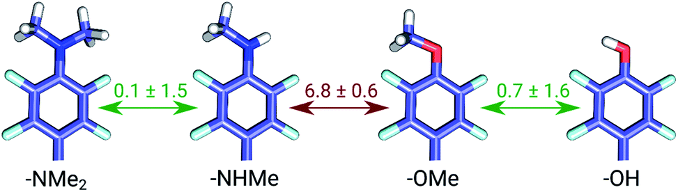
Double free energy differences (ΔΔG) were calculated for a set of 482 ligand modifications across 13 protein–ligand datasets. This large set of diverse modifications allows for a reliable comparison between the investigated alchemical approaches. Fig. 1A summarizes the main findings: in absolute terms (average unsigned error, AUE), the pmx-based non-equilibrium free energy calculations perform equivalently to the state-of-the-art FEP+ approach. Predictions of both approaches, on average, deviate from experiment by less than 1 kcal mol⁻¹ (4.184 kJ mol⁻¹). The individual force fields, GAFF and CGenFF, are outperformed by FEP+ using the proprietary OPLSv3 force field. However, remarkably, the combination of free energy estimates obtained with GAFF and CGenFF force fields (even when considering equivalent sampling time) substantially improves the accuracy. The agreement with experiment in terms of Pearson correlation is slightly better for the FEP+ approach (0.69 ± 0.03) than for the consensus force field approach based on the non-equilibrium free energy calculations (0.63 ± 0.03). Similar to the AUE comparison, in terms of Pearson correlation, the consensus force field approach appears to yield higher quality estimates than the individual force fields, when considering all protein–ligand datasets together.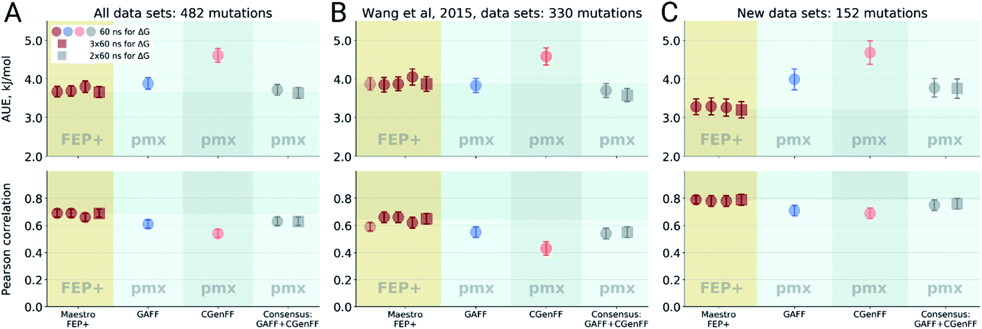

Fig. 1 Average unsigned errors (AUE, upper plots) and correlations (lower plots) between the calculated and experimentally measured double free energy differences. In the FEP+ panels, the dark red circles represent the three separate replica calculations, and the dark red square the results when the ΔΔG values per ligand are averaged over the three replicas. For the pmx GAFF and CGenFF panels, the circle symbols denote results averaged over three replicas (60 ns per ΔG in total). In the consensus panel, the results were averaged to correspond to 60 ns (circle) and 2 × 60 ns (square) of sampling time per ΔG estimate. (A) Averaging performed over all the investigated protein–ligand complexes; 482 ligand modifications in total. (B) Subset of systems analyzed by Wang et al.;³ 330 ligand modifications. The light red circle in this panel corresponds to the result reported by Wang et al. (C) Subset of systems added in this work; 152 ligand modifications.

The comparisons described above took into consideration all the simulations performed for each approach, i.e. a total of 3 × 60 ns for every ΔG estimate with FEP+, and 2 × 60 ns (i.e. 60 ns for each force field, GAFF and CGenFF: in total, 6 replicas of 20 ns each were combined for a ΔG estimate) for the pmx-based free energy calculations. When considering the equivalent time of 60 ns per ΔG value, the accuracies obtained by both approaches are nearly identical: FEP+ returns an AUE of 3.72 ± 0.15 kJ mol⁻¹ and a correlation of 0.68 ± 0.03; the consensus force field pmx calculations yield an AUE of 3.72 ± 0.15 kJ mol⁻¹ and a correlation of 0.63 ± 0.03.

The dataset analyzed in Fig. 1A can be decomposed into two subsets: the set of 8 protein–ligand systems (330 mutations) assembled and analyzed by Wang et al.³ and an additional set of 5 protein–ligand systems comprising 152 mutations. Wang et al. used an earlier version of the OPLS force field (v2.1) to investigate the subset of 330 mutations, thus, it is interesting to compare the evolution of the FEP+ method and force field with the accuracy of the open-source pmx-based calculations (Fig. 1B). Wang et al. reported an AUE of 3.87 ± 0.17 kJ mol⁻¹. Subsequently, Harder et al. reported an improved AUE of 3.36 ± 0.15 kJ mol⁻¹ for the same 8 protein–ligand systems with the OPLSv3 force field.⁸⁸ However, the simulation time used for obtaining the latter result is not reported, complicating a direct comparison. In the current work, using FEP+ with the OPLSv3 force field and combining free energy estimates from three independent FEP+ runs resulted in an AUE of 3.66 ± 0.14 kJ mol⁻¹. The non-equilibrium free energy calculations performed comparably to FEP+ and reached an AUE of 3.70 ± 0.17 kJ mol⁻¹ when using 60 ns per ΔG estimate, and 3.58 ± 0.18 kJ mol⁻¹ when using 2 × 60 ns. In terms of correlation, the newer OPLSv3 shows improvement over OPLSv2.1: 0.65 ± 0.04 versus 0.59 ± 0.03. The pmx-based calculations show slightly lower correlation of 0.55 ± 0.04. In a recent study, the Wang et al. dataset was investigated with equilibrium TI calculations using the Amber18 simulation package.⁸⁹ The authors reported substantially worse performance than obtained in the current work: AUE of 4.9 kJ mol⁻¹ and correlation of 0.48, investing 74 ns per ΔG estimate.

For the dataset of 152 mutations (Fig. 1C) assembled from the literature for this study, both FEP+ and non-equilibrium calculations reach similar correlation: 0.79 ± 0.04 and 0.76 ± 0.04, respectively. Interestingly, for this subset the AUE of the FEP+ predictions is lower than that of the consensus approach by 0.57 ± 0.33 kJ mol⁻¹ (3.2 ± 0.21 and 3.77 ± 0.25 kJ mol⁻¹ for FEP+ and pmx, respectively). These observations suggest the accuracy is dependent on the particular protein–ligand system studied. It is also important to note that the number of data points varies among the datasets, ranging from 7 in the case of galectin, to 71 in the case of MCL1. This emphasizes the importance of using large datasets for reliable method comparison.

For all the sets depicted in Fig. 1, the GAFF force field outperforms CGenFF. Combining the results of both into a consensus estimate consistently yields a higher, or at least equivalent, accuracy compared to the GAFF force field. Increasing the simulation time invested to obtain a ΔΔG estimate has only a marginal effect on the results, given the time scales considered (at least 60 ns per ΔG). We have also probed the effect of simulation length on FEP+ accuracy by running 1 ns per λ window and using 3 replicas, resulting in 36 ns per ΔG estimate, as opposed to the standard protocol using 5 ns per λ window (180 ns per ΔG). Also in this case, the accuracy was only marginally affected by the shorter simulations: AUE of 3.88 ± 0.15 (1 ns) and 3.66 ± 0.14 kJ mol⁻¹ (5 ns), and correlation 0.68 ± 0.03 and 0.69 ± 0.03, respectively.

To further assess the sensitivity of the GROMACS calculations to the invested sampling time, we estimated ΔΔG values after discarding half of the simulation time. Such a protocol resulted in a setup using 3 replicas of 10 ns, which closely matches the 1 ns FEP+ protocol (1 ns × 12 λ-windows × 3 replicas). The AUE of the GAFF calculations was 4.03 ± 0.16 kJ mol⁻¹ and the Pearson correlation 0.59 ± 0.03. The CGenFF calculations had an AUE of 4.7 ± 0.19 kJ mol⁻¹ and correlation of 0.53 ± 0.04. The modest decrease in accuracy matches well with the similar effect observed for the FEP+ calculations. It appears that even the shorter investigated sampling times are sufficient to explore the local minima in the vicinity of the starting structure to obtain a converged free energy estimate. This is corroborated by our earlier explorations of sampling strategies applied in drug resistance mutation studies, where investing 54 ns per ΔG value yielded converged results.³⁵

The scatter plots of the calculated and experimental double free energy differences provide an intuitive understanding of the ranges spanned by the datasets and the calculated values (Fig. 2). While taken separately the GAFF and CGenFF force fields produce more outliers than FEP+ with OPLSv3 (Fig. 2 and S1‡), the consensus results reduce the number of outliers. The proportion of estimates falling within 1 kcal mol⁻¹ (4.184 kJ mol⁻¹) of experiment is 68 ± 2% and 66 ± 2% for the FEP+ and the pmx-based consensus force field approach respectively. The overall range spanned by the estimated ΔΔG values is comparable between the methods and force fields as well as similar to the distribution of experimental values (Fig. S2‡). The consensus non-equilibrium estimates were more accurate than FEP+ for the perturbations associated with a small ΔΔG (Fig. S4‡), whereas FEP+ was more accurate for larger ΔΔG perturbations.

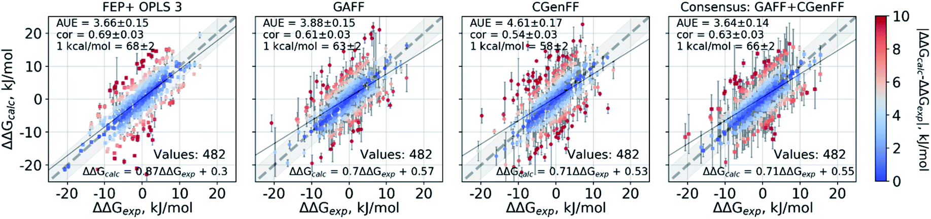Fig. 2 Calculated ΔΔG values plotted against the experimental measurements considering all 482 ligand modifications investigated in this work. The FEP+ calculations used 3 replicas of 60 ns each for every ΔG estimate. The pmx-based calculations with GAFF and CGenFF used 3 replicas of 20 ns each, i.e. summing to 60 ns per ΔG estimate. The consensus results shown here use 2 × 60 ns per ΔG estimate. Text in the panels: AUE is in kJ mol⁻¹; “cor” is Pearson correlation; “1 kcal/mol” denotes the percentage of the estimates that fall within 1 kcal mol⁻¹ (4.184 kJ mol⁻¹) of the experimental measurement; “values” refers to the total number of perturbations.

A notable difference between the results of the methods is the magnitude of estimated errors (Fig. 2 and S3‡): the non-equilibrium free energy estimates have larger associated errors than those predicted by FEP+. It is important to note that error estimates for the individual ΔΔG values comprise both the uncertainty of the estimator and the standard error of the estimates coming from the different simulation replicas. Furthermore, the consensus approach increases the errors because the GAFF and CGenFF estimates may differ from each other more than the estimates obtained with individual force fields. While this feature allows for an increased prediction accuracy, it also increases the uncertainty associated with an estimate.

Case-by-case analysis

The agreement between the free energy predictions and experiment is system dependent. Fig. 3 summarizes the AUE and Pearson correlation for every protein–ligand complex studied (Fig. S8‡ shows average signed errors). Together with the system-dependent accuracy, Fig. 3 again highlights the value of the consensus force field approach. In several cases the ΔΔG estimate between force fields varies greatly, leading to substantially different AUEs (CGenFF shows larger AUEs for one of the BACE sets, TYK2, MCL1, and P38, while GAFF for cMET). This is also the case for the Pearson correlation. Taking the consensus of the estimated free energy differences by using a simple average of the values from the two force fields yields a result outperforming or on par with the best result from a single force field.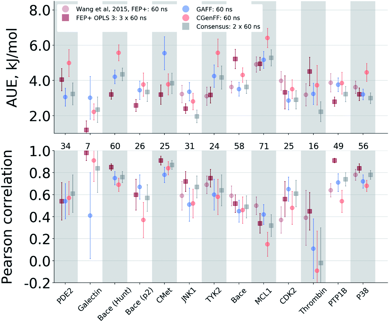

Fig. 3 Average unsigned error (AUE) and Pearson correlation for the ΔΔG estimates split by protein–ligand system. The numbers in between the top and bottom panels denote the number of ligand modifications considered for the corresponding system.

The improved accuracy due to combination of results from different force fields may seem counterintuitive. In fact, if both force fields yield ΔΔG estimates deviating from experiment in the same direction, the consensus approach would yield only an intermediate quality prediction falling in between the two individual force fields. Such an outcome would still be preferable in a prospective study, since relying on a single force field might lead the investigation in a wrong direction. In the current work, however, employing a consensus approach generally resulted in an improved prediction accuracy over any of the single force fields. This is only possible because in 33% of all the calculated double free energy differences the values obtained by GAFF and CGenFF force fields were pointing in opposite directions from the experimental measurement (see also Fig. S10‡ for a graphical depiction of the signed deviations from experiment for both force fields plotted one against the other).

The variable performance of calculated ΔΔG for individual protein–ligand complexes can be seen from the scatter plots in Fig. 4 (for the FEP+ estimates see Fig. S6‡). In the majority of cases, the estimates fall within 1 kcal mol⁻¹ (4.184 kJ mol⁻¹) of the experimental measurement. This indicates that the accuracy is mainly reduced by a small number of outliers. The latter observation holds for both the consensus approach based on the non-equilibrium calculations (Fig. 4) and FEP+ using the OPLSv3 force field (Fig. S6‡). Interestingly, both approaches have difficulties with the MCL1 dataset where only half of the estimates fall within 1 kcal mol⁻¹ (4.184 kJ mol⁻¹) of the experimental measurement. 45% of the non-equilibrium estimates fell outside this range for the BACE set of Hunt et al.⁶⁴ and for the cMET set. FEP+ had comparable difficulties with the BACE set of Cumming et al.⁹⁰ and PDE2.³³

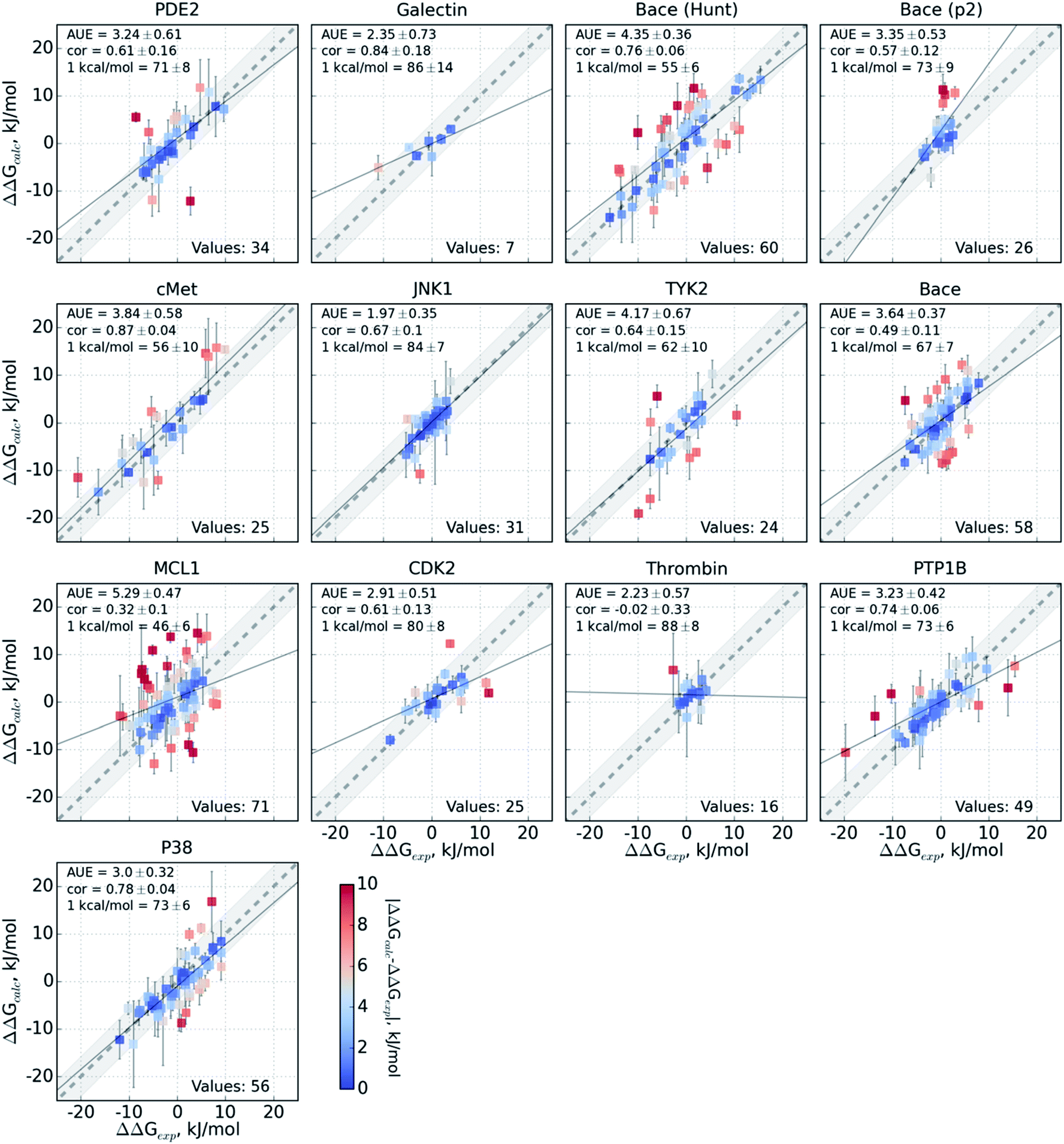Fig. 4 Performance of the pmx-based consensus force field calculations for each protein–ligand system studied. The ΔΔG estimates are plotted against their experimentally determined values. Text in the panels: AUE is in kJ mol⁻¹; “cor” is Pearson correlation; “1 kcal/mol” denotes the percentage of the estimates that fall within 1 kcal mol⁻¹ (4.184 kJ mol⁻¹) of the experimental measurement; “values” refers to the total number of perturbations per dataset.

The range spanned by the ΔΔG values also has an influence on the prediction accuracy (Fig. S5‡). An illustrative example for this effect is a set of thrombin inhibitors. The experimental range of the double free energy differences is narrow. The non-equilibrium approach captured the ΔΔG values very accurately in terms of AUE (2.23 ± 0.57 kJ mol⁻¹). However, no correlation for the small differences between the ligands was observed. In contrast, FEP+ had a significantly larger AUE of 4.51 ± 0.82 kJ mol⁻¹. However, it was able to achieve moderate correlation (0.45 ± 0.18). In general, FEP+ obtained higher correlations: the averaged correlation coefficient was higher for 9 out of 13 datasets (Fig. S7‡). In terms of AUE, on average, FEP+ was more accurate than the pmx-based calculations for 7 out of 13 datasets. When compared to the previous generation of the OPLS force field (v2.1),³ the consensus force field approach performs better in 6 out of 8 cases in terms of AUE and 3/8 in terms of correlation. It is worth noting that the earlier FEP+ results reported by Wang et al. were more accurate for BACE and thrombin than those obtained here with the newer OPLS version.

Determinants of prediction accuracy

Protonation effects. For one system (PTP1B), we looked in detail at the molecular determinants influencing the free energy calculation accuracy. In particular, we investigated the effects of the protonation state of the catalytic cysteine. PTP1B is a tyrosine phosphatase that harbors a catalytic cysteine (Cys215) that can be oxidized, thus inhibiting the enzyme.⁹¹ When in the apo state, Cys215 has been shown to be deprotonated (pK_a = 5.4) and make a covalent bond with the main chain nitrogen of Ser216.⁹² The protonation state of Cys215 is not known for the set of PTP1B inhibitors probed here. From the crystallographic structures resolved with four of the ligands in the set,⁹³ the short distance between the cysteine's sulfur and the closest carboxyl group oxygen of a ligand (3.5–3.9 Å) suggests a possible formation of a weak hydrogen bond (Fig. 5).

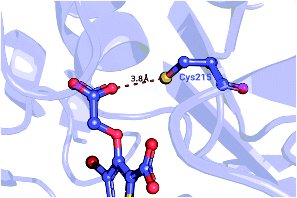Fig. 5 Detail of a PTP1B structure (PDB ID: 2qbs) depicting the close proximity of the thiol group of Cys215 to the carboxyl group of the co-crystallized inhibitor.

We further probed whether the ligand's carboxyl group or Cys215 is more likely to be protonated. The empirical pK_a predictor PROPKA 3.1 ^94,95 suggested that the pK_a for the carboxyl group is less than 5.0 for every ligand in the set. The low carboxyl pK_a was also confirmed by the ChemAxon's predictor.⁹⁶ In contrast, the pK_a for Cys215 in the complexed system was predicted to be between 9.8 and 10.5, depending on the inhibitor. Taken together, these observations suggest that Cys215 ought to be protonated for the inhibitor set synthesized by Wilson et al.⁹³

Wang et al.,³ however, modeled a deprotonated variant of Cys215 in their free energy calculations, whilst also keeping the ligand's carboxyl group deprotonated. Although the carboxyl groups of the ligand are not modified in the alchemical simulations it is plausible that structurally diverse inhibitors may be affected differently by the two negative charges nearby. Using the Wang et al. setup with the deprotonated Cys215 we obtained similar quality free energy estimates (Fig. 6). Briefly, the Cys(−1) results from Wang et al. had an AUE and correlation of 3.87 ± 0.52 kJ mol⁻¹ and 0.64 ± 0.06, respectively, compared to 3.66 ± 0.56 kJ mol⁻¹ and 0.61 ± 0.08 from the pmx consensus predictions, also with similar outliers as seen in the correlation plots. Interestingly, the FEP+ calculations performed here using OPLSv3 showed substantially better accuracy (AUE of 2.8 ± 0.27 kJ mol⁻¹ and correlation of 0.91 ± 0.03), suggesting the newer force field includes updates that have an improved representation of interactions between the deprotonated thiol and carboxyl group for the investigated set of ligands. Since our empirical prediction suggests that Cys215 could be protonated we have also calculated free energy differences with this protonation state. Interestingly, upon protonation of Cys215 the quality of FEP+ OPLSv3 prediction drops (Fig. 6): AUE 3.68 ± 0.49 kJ mol⁻¹, correlation 0.8 ± 0.07.

Fig. 6 Details of the ΔΔG calculations for the PTP1B protein–ligand system. The top row depicts the experimental ΔΔG values plotted against the calculated results. The two bottom panels summarize these calculations in terms of AUE and Pearson correlation. From left to right: Wang et al.³ calculations using deprotonated Cys215; FEP+ with OPLS v3 using deprotonated Cys215; FEP+ with OPLS v3 with protonated Cys215; pmx-based consensus force field approach with deprotonated Cys215; pmx-based consensus force field approach with deprotonated, but neutral Cys215; pmx-based consensus force field approach with protonated Cys215.

The pmx calculations using the consensus force field approach follow a different trend. When Cys215 is deprotonated and turned into a neutral residue (by redistributing charges on the side-chain atoms), the agreement with experiment increases. This artificially constructed cysteine residue should not be interpreted in physical terms (e.g. as a radical). It rather represents a convenient intermediate step between the negative deprotonated cysteine in the active site of PTP1B and the properly protonated neutral Cys215. Agreement with experiment further improves when Cys215 is protonated (Fig. 6): AUE 3.23 ± 0.42 kJ mol⁻¹, correlation 0.74 ± 0.06. The increased accuracy when protonating Cys215 could be an artifact of a deficient parameterization of the thiolate group in Amber and CHARMM force fields.⁹⁷ On the other hand, it may also suggest that the thiol group of the cysteine residue is protonated upon binding of the ligands from the investigated set of PTP1B inhibitors.

It is also important to note that here we only analyzed the effects of protonation changes of the cysteine's thiol group, while the protonation state of the ligands was kept fixed. For a complete picture of the free energy landscape underlying the affinity differences for this PTP1B ligand set it might be necessary to include alternative protonation states for the ligands^98,99 and potentially allow the molecules to change their protonation upon binding. Although in the current analysis we verified ligand protonation states by means of empirical predictors, future systematic free energy calculations including ligand protonation effects may improve estimation accuracy.

Sensitivity to ligand parameterization. Disentangling the reasons underlying the quality of free energy calculation performance is not a trivial task. On the one hand inaccuracies frequently arise due to insufficient sampling. While this can be circumvented by increasing simulation time or adding more replicas, the problem of imperfect force field parameterization represents another major source of errors. The calculated free energies integrate contributions from the protein force field, ligand parameterization and water model, all of which are prone to introducing errors that may lead to unexpected outcomes. The galectin data set serves as an example for such effects.

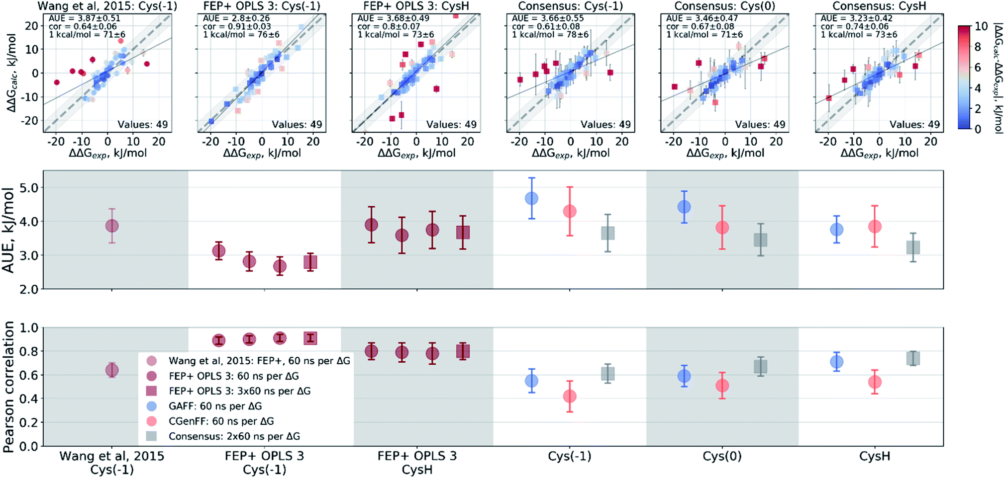
The set of galectin inhibitors contains only 8 ligands connected by 7 perturbations. OPLSv3 performed particularly well in this case: AUE of 1.2 ± 0.5 kJ mol⁻¹, correlation of 0.98 (Fig. 3). Both GAFF and CGenFF force fields show a lower accuracy in terms of AUE (3.0 ± 1.2 and 2.2 ± 0.4 kJ mol⁻¹, respectively). In terms of correlation, GAFF has a below-average agreement with experiment and a large associated uncertainty (0.41 ± 0.4). A closer look into the ΔΔG estimates obtained with the GAFF force field highlights a peculiar case of possible error cancellation in the free energy estimates (Fig. 7). A large AUE for the perturbation transforming a methylamino group (–NHMe) to methoxy (–OMe) suggests that the parameterization of one or both of these moieties might be imperfect. However, perturbations of these groups into more chemically similar substituents gave more accurate ΔΔG estimates: methylamine to di-methylamine; methoxy to hydroxyl. The parameterization errors pertaining to a specific chemical group cancel out until transformations involving different chemistry (with different parameterization errors) are introduced: e.g. free energy differences within the group of ligands containing methylamine in the current case are represented correctly. Similarly, the free energy differences within the group of compounds containing methoxy and hydroxyl groups are accurately estimated. However, the free energy difference between these two sets of ligands containing different chemical groups is not captured accurately (at least not with the sampling time used in the current study).

Fig. 7 Average unsigned errors (AUE) for perturbations in the galectin data set using GAFF force field. Values are in kJ mol⁻¹.

Directions for force field optimization. The consensus force field approach provided more accurate predictions than the individual GAFF and CGenFF force fields. As already mentioned, an improvement in accuracy is only possible if the two force field estimates are opposite with respect to the experimental result. The cMet protein–ligand dataset provides an informative example: in 14 out of 25 (56%) cases GAFF and CGenFF predictions had an error in different directions from the experimental measurement. The cMet inhibitor set contains 12 ligands with a common scaffold (Fig. 8A) and a single substitution site (Fig. 8B), except for compound 1_21, which also has a cyano group in place of a scaffold fluorine atom. Overall, for this system FEP+ showed an AUE of 3.2 ± 0.58 kJ mol⁻¹, while CGenFF was only slightly worse with an AUE of 3.78 ± 0.59 kJ mol⁻¹. Interestingly, this dataset gave the worst performance for GAFF among all the investigated protein–ligand complexes: AUE of 5.55 ± 0.94 kJ mol⁻¹.

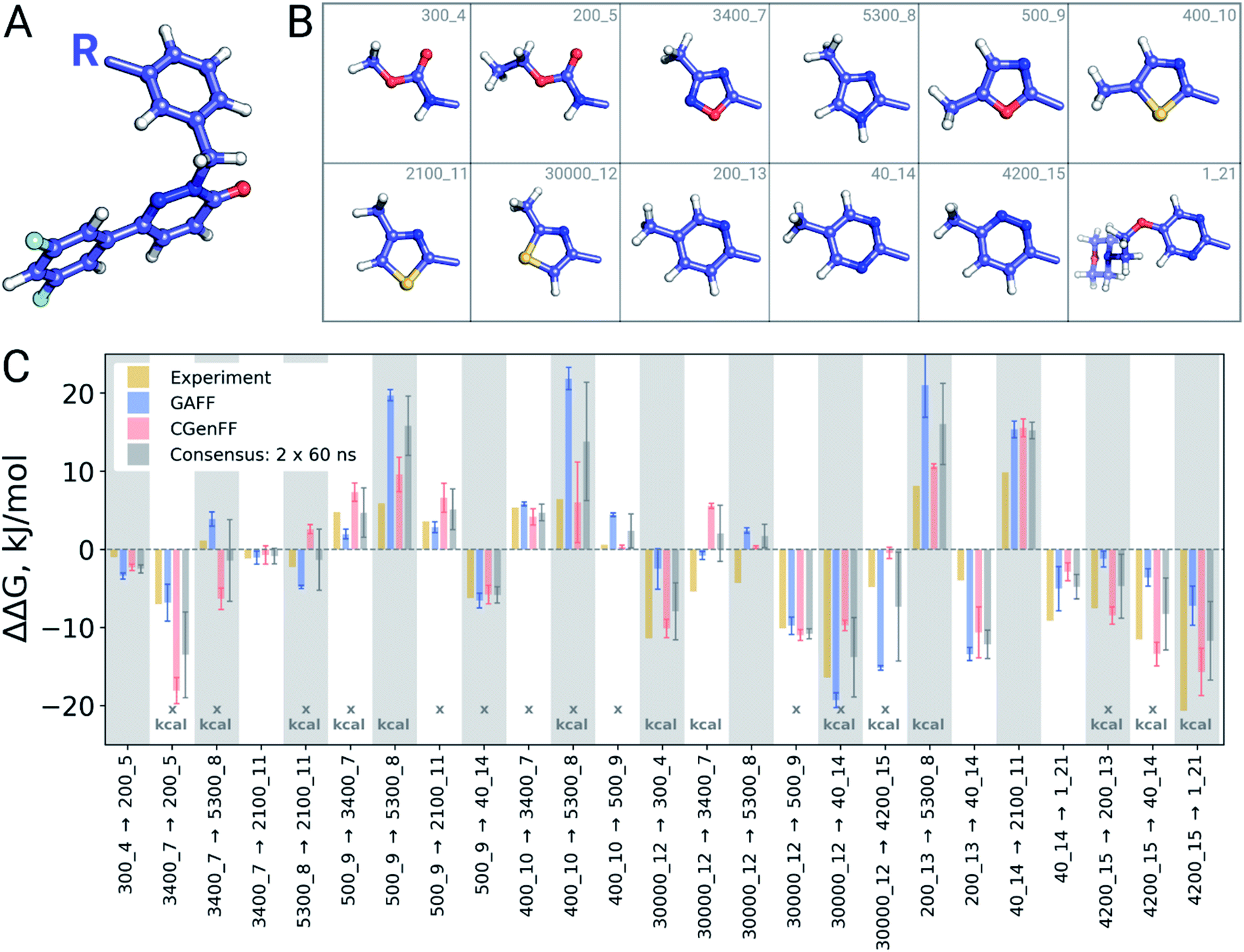Fig. 8 cMet inhibitor dataset. (A) Common scaffold of the compounds. (B) Substituents for the 12 cMet inhibitors. (C) ΔΔG for the transformations. The cases where GAFF and CGenFF results point in the opposite direction from the experiment are marked with an “x”, while differences between the force field results larger than 1 kcal mol⁻¹ (4.184 kJ mol⁻¹) are marked with “kcal”.

A closer look at the major discrepancies between force fields reveals some peculiar trends that could be useful for further force field fine tuning. For example, in all four transformations with compound 4200_15, GAFF overestimates the binding affinity of this ligand in comparison to both CGenFF and experiment. Similarly, compound 400_10 is consistently (3 transformations) predicted by GAFF to be a higher affinity binder than determined experimentally. In contrast, all 6 transformations involving ligand 5300_8 with GAFF suggest the inhibitor to be a far worse binder than measured experimentally. Although pinpointing the exact force field parameters that are responsible for these inaccuracies is not trivial, the trends observed for certain chemical groups suggest likely candidates for re-parameterization. Similarly, we can envisage future work using large-scale scans of such calculated thermodynamic properties of biomolecular complexes to aid force field development.

Discussion

Overall, the current investigation revealed several consistent trends. The accuracy in terms of AUE was comparable for the FEP+ and pmx-based calculations, while the correlation was slightly higher for FEP+ when using the OPLSv3 force field (Fig. 1). The GAFF force field yielded higher accuracy than CGenFF, however, the consensus approach of averaging the results from both force fields performed better or equally well as the best performing force field. This indicates that the errors made by the force fields in free energy estimates are in some cases cancelling out, allowing for an increased accuracy. This effect has been previously observed in the free energy estimations for amino acid mutations in protein stability and protein–ligand binding studies,^27,35 as well as for nucleotide mutations in protein–DNA interactions.²⁹ Furthermore, the benefits of the consensus approach are emphasized in the case-by-case analysis of the protein–ligand complexes studied (Fig. 3). Here, it becomes evident that in a prospective study of a particular system relying on the results of a single force field may lead to a substantial decrease in the predictive accuracy. In fact, in the current investigation, the two force fields gave opposite results with respect to experiment for as many as 33% of the cases, while in 10% of the cases the estimates from two force fields showed a statistically significant systematic difference. Admittedly, using a consensus approach requires additional effort in preparing the simulation system. With the currently available software packages,^68,71 however, automation of such procedures should not pose a considerable challenge.

The significant difference in standard errors obtained from repeated calculations represents an interesting difference between the FEP+ and non-equilibrium TI based free energy results. With an average standard error of 0.57 kJ mol⁻¹ per ΔΔG value, FEP+ provides predictions with high precision. That is, the ΔΔG estimates from FEP+ converge to highly similar values, with little spread in the results. This might be a consequence of the enhanced sampling technique (REST⁶⁵) ensuring convergence of the FEP+ simulations. pmx-based non-equilibrium calculations, on the other hand, come with higher uncertainty: 2.36 kJ mol⁻¹ on average for the consensus results. The larger spread of the calculated ΔΔG values, in comparison to FEP+, suggests that the non-equilibrium calculations could still benefit from an increased convergence: longer simulations or an enhanced sampling approach present a compelling direction for further investigation. Considering that both FEP+ and pmx-based calculations have, on average, a similar AUE of ∼3.7 kJ mol⁻¹, the high precision associated with FEP+ indicates that the method is highly precise even for those predictions that are substantially different from experiment. The pmx-based calculations give a larger prediction uncertainty, thus encompassing the experimental observation within the confidence interval of the estimate. It remains to be explored whether increased precision of the pmx-based calculations (using longer simulations or an enhanced sampling technique) will have an effect on the accuracy of free energy estimates.

The success of combining results from GAFF and CGenFF indicates differences in the force field parameterization. Naturally, the simplistic forms of the potential energy functions used by the classical molecular mechanics force fields cannot capture the full complexity of molecular interactions, for which a more complex representation would be required, e.g., polarizability.^100,101 Force field parameterization based on a large number of quantum chemical calculations is helpful, as illustrated by the high accuracy achieved by FEP+ with the OPLSv3 force field. However, the simplified description of the potential energy leads to unavoidable, inherent limitations. Thus, at this time, combining estimates from different force fields may be an attractive avenue to pursue. Given that parameterization of different force fields relies on different theoretical premises, combining their results may indirectly capture features of molecular interactions that are inaccessible to a single force field. Finally, the significant prediction differences obtained when altering the protonation state of a single amino acid sidechain highlight the sensitivity of alchemical methods to the simulation setup and force field parameterization details. Furthermore, this example emphasizes the need for transparent and open-source force field parameters akin to those put forward by the Open Force Field Consortium.¹⁰²

Conclusions

In the current investigation, we have demonstrated that a non-equilibrium free energy calculation method based on freely available open-source software performs on par with state-of-art commercial software. The results obtained from a large-scale protein–ligand relative binding affinity scan highlight an improvement in accuracy when combining results from multiple force fields into a consensus estimate. The presented approach is readily applicable in drug discovery lead optimization projects. Descriptive workflows, comprising the technical steps required for the free energy calculations, will further provide an easy-to-use approach for ligand–protein binding affinity prediction.

Author contributions

The manuscript was written through contributions of all authors. All authors have given approval to the final version of the manuscript.

Conflicts of interest

There are no conflicts to declare.

Acknowledgements

We thank Dr James P. Edwards for reviewing the manuscript and the GROMACS development team for making their software freely available. L. P. B. was partly funded by the European Union's Horizon 2020 Research and Innovation Programme under grant agreement No 675451 (CompBioMed project). The project was also partly funded by Vlaams Agentschap Innoveren & Ondernemen Project 155028. V. G. and B. L. d. G. were supported by the BioExcel CoE (http://www.bioexcel.eu), a project funded by the European Union (Contract H2020-EINFRA-2015-1-675728). M. A. was supported by a Postdoctoral Research Fellowship of the Alexander von Humboldt Foundation.

References

1. G. L. Warren, C. W. Andrews, A.-M. Capelli, B. Clarke, J. LaLonde, M. H. Lambert, M. Lindvall, N. Nevins, S. F. Semus, S. Senger, G. Tedesco, I. D. Wall, J. M. Woolven, C. E. Peishoff and M. S. Head, J. Med. Chem., 2006, 49, 5912–5931.
2. G. Sliwoski, S. Kothiwale, J. Meiler and E. W. Lowe, Pharmacol. Rev., 2014, 66, 334–395.
3. L. Wang, Y. Wu, Y. Deng, B. Kim, L. Pierce, G. Krilov, D. Lupyan, S. Robinson, M. K. Dahlgren, J. Greenwood, D. L. Romero, C. Masse, J. L. Knight, T. Steinbrecher, T. Beuming, W. Damm, E. Harder, W. Sherman, M. Brewer, R. Wester, M. Murcko, L. Frye, R. Farid, T. Lin, D. L. Mobley, W. L. Jorgensen, B. J. Berne, R. A. Friesner and R. Abel, J. Am. Chem. Soc., 2015, 137, 2695–2703.
4. D. Plewczynski, M. Łaźniewski, R. Augustyniak and K. Ginalski, J. Comput. Chem., 2011, 32, 742–755.
5. W. L. Jorgensen, Acc. Chem. Res., 2009, 42, 724–733.
6. M. De Vivo, M. Masetti, G. Bottegoni and A. Cavalli, J. Med. Chem., 2016, 59, 4035–4061.
7. Z. Cournia, B. Allen and W. Sherman, J. Chem. Inf. Model., 2017, 57, 2911–2937.
8. R. W. Zwanzig, J. Chem. Phys., 1954, 22, 1420–1426.
9. C. H. Bennett, J. Comput. Phys., 1976, 22, 245–268.
10. J. G. Kirkwood, J. Chem. Phys., 1935, 3, 300–313.
11. J. A. McCammon, B. R. Gelin and M. Karplus, Nature, 1977, 267, 585–590.
12. W. L. Jorgensen and C. Ravimohan, J. Chem. Phys., 1985, 83, 3050–3054.
13. P. Kollman, Chem. Rev., 1993, 93, 2395–2417.
14. C. F. Wong and J. A. McCammon, J. Am. Chem. Soc., 1986, 108, 3830–3832.
15. K. M. Merz Jr and P. A. Kollman, J. Am. Chem. Soc., 1989, 111, 5649–5658.
16. T. C. Beutler, A. E. Mark, R. C. van Schaik, P. R. Gerber and W. F. van Gunsteren, Chem. Phys. Lett., 1994, 222, 529–539.
17. M. Zacharias, T. P. Straatsma and J. A. McCammon, J. Chem. Phys., 1994, 100, 9025–9031.
18. V. Gapsys, D. Seeliger and B. L. de Groot, J. Chem. Theory Comput., 2012, 8, 2373–2382.
19. M. J. Harvey, G. Giupponi and G. D. Fabritiis, J. Chem. Theory Comput., 2009, 5, 1632–1639.
20. A. W. Götz, M. J. Williamson, D. Xu, D. Poole, S. Le Grand and R. C. Walker, J. Chem. Theory Comput., 2012, 8, 1542–1555.
21. R. Abel, L. Wang, E. D. Harder, B. Berne and R. A. Friesner, Acc. Chem. Res., 2017, 50, 1625–1632.
22. K. J. Bowers, D. E. Chow, H. Xu, R. O. Dror, M. P. Eastwood, B. A. Gregersen, J. L. Klepeis, I. Kolossvary, M. A. Moraes, F. D. Sacerdoti, J. K. Salmon, Y. Shan and D. E. Shaw, SC '06: Proceedings of the 2006 ACM/IEEE Conference on Supercomputing, 2006.
23. C. D. Christ and T. Fox, J. Chem. Inf. Model., 2014, 54, 108–120.
24. P. Mikulskis, S. Genheden and U. Ryde, J. Chem. Inf. Model., 2014, 54, 2794–2806.
25. F. J. Rombouts, G. Tresadern, P. Buijnsters, X. Langlois, F. Tovar, T. B. Steinbrecher, G. Vanhoof, M. Somers, J.-I. Andrés and A. s. A. Trabanco, ACS Med. Chem. Lett., 2015, 6, 282–286.
26. M. Ciordia, L. Pérez-Benito, F. Delgado, A. A. Trabanco and G. Tresadern, J. Chem. Inf. Model., 2016, 56, 1856–1871.
27. V. Gapsys, S. Michielssens, D. Seeliger and B. L. de Groot, Angew. Chem., Int. Ed., 2016, 55, 7364–7368.
28. H. Keränen, L. Pérez-Benito, M. Ciordia, F. Delgado, T. B. Steinbrecher, D. Oehlrich, H. W. van Vlijmen, A. s. A. Trabanco and G. Tresadern, J. Chem. Theory Comput., 2017, 13, 1439–1453.
29. V. Gapsys and B. L. de Groot, J. Chem. Theory Comput., 2017, 13, 6275–6289.
30. B. Kuhn, M. Tichy, L. Wang, S. Robinson, R. E. Martin, A. Kuglstatter, J. r. Benz, M. Giroud, T. Schirmeister and R. Abel, J. Med. Chem., 2017, 60, 2485–2497.
31. V. Wagner, L. Jantz, H. Briem, K. Sommer, M. Rarey and C. D. Christ, ChemMedChem, 2017, 12, 1866–1872.
32. J. Z. Vilseck, K. A. Armacost, R. L. Hayes, G. B. Goh and C. L. Brooks, J. Phys. Chem. Lett., 2018, 9, 3328–3332.
33. L. Pérez-Benito, H. Keränen, H. van Vlijmen and G. Tresadern, Sci. Rep., 2018, 8, 4883.
34. T. Bastys, V. Gapsys, N. T. Doncheva, R. Kaiser, B. L. de Groot and O. V. Kalinina, J. Chem. Theory Comput., 2018, 14, 3397–3408.
35. M. Aldeghi, V. Gapsys and B. L. de Groot, ACS Cent. Sci., 2018, 4, 1708–1718.
36. L. Pérez-Benito, N. Casajuana-Martin, M. Jiménez-Rosés, H. van Vlijmen and G. Tresadern, J. Chem. Theory Comput., 2019, 15, 1884–1895.
37. M. Lundborg and E. Lindahl, J. Phys. Chem. B, 2015, 119, 810–823.
38. L. S. Dodda, I. Cabeza de Vaca, J. Tirado-Rives and W. L. Jorgensen, Nucleic Acids Res., 2017, 45, W331–W336.
39. V. Zoete, M. A. Cuendet, A. Grosdidier and O. Michielin, J. Comput. Chem., 2011, 32, 2359–2368.
40. H. H. Loeffler, J. Michel and C. Woods, J. Chem. Inf. Model., 2015, 55, 2485–2490.
41. H. Fu, J. C. Gumbart, H. Chen, X. Shao, W. Cai and C. Chipot, J. Chem. Inf. Model., 2018, 58, 556–560.
42. P. V. Klimovich and D. L. Mobley, J. Comput.-Aided Mol. Des., 2015, 29, 1007–1014.
43. V. Ramadoss, F. Dehez and C. Chipot, J. Chem. Inf. Model., 2016, 56, 1122–1126.
44. S. Liu, Y. Wu, T. Lin, R. Abel, J. P. Redmann, C. M. Summa, V. R. Jaber, N. M. Lim and D. L. Mobley, J. Comput.-Aided Mol. Des., 2013, 27, 755–770.
45. P. V. Klimovich, M. R. Shirts and D. L. Mobley, J. Comput.-Aided Mol. Des., 2015, 29, 397–411.
46. V. Gapsys, S. Michielssens, D. Seeliger and B. L. de Groot, J. Comput. Chem., 2015, 36, 348–354.
47. V. Gapsys and B. L. de Groot, J. Chem. Inf. Model., 2017, 57, 109–114.
48. M. R. Shirts and D. L. Mobley, in Biomolecular Simulations: Methods and Protocols, ed. L. Monticelli and E. Salonen, Humana Press, Totowa, NJ, 2013, pp. 271–311,  DOI:10.1007/978-1-62703-017-5_11.
49. M. J. Abraham, T. Murtola, R. Schulz, S. Páll, J. C. Smith, B. Hess and E. Lindahl, SoftwareX, 2015, 1–2, 19–25.
50. D. Seeliger and B. L. de Groot, Biophys. J., 2010, 98, 2309–2316.
51. A. W. Yee, M. Aldeghi, M. P. Blakeley, A. Ostermann, P. J. Mas, M. Moulin, D. de Sanctis, M. W. Bowler, C. Mueller-Dieckmann, E. P. Mitchell, M. Haertlein, B. L. de Groot, E. Boeri Erba and V. T. Forsyth, Nat. Commun., 2019, 10, 925.
52. S. Michielssens, J. H. Peters, D. Ban, S. Pratihar, D. Seeliger, M. Sharma, K. Giller, T. M. Sabo, S. Becker, D. Lee, C. Griesinger and B. L. de Groot, Angew. Chem., Int. Ed., 2014, 53, 10367–10371.
53. G. E. Crooks, Phys. Rev. E: Stat. Phys., Plasmas, Fluids, Relat. Interdiscip. Top., 1999, 60, 2721–2726.
54. F. M. Ytreberg, R. H. Swendsen and D. M. Zuckerman, J. Chem. Phys., 2006, 125, 184114.
55. M. Goette and H. Grubmüller, J. Comput. Chem., 2009, 30, 447–456.
56. A. Yildirim, T. A. Wassenaar and D. v. d. Spoel, J. Chem. Phys., 2018, 149, 144111.
57. P. Procacci, J. Chem. Phys., 2019, 150, 127101.
58. V. Gapsys, S. Michielssens, J. H. Peters, B. L. de Groot and H. Leonov, in Molecular Modeling of Proteins, ed. A. Kukol, Springer New York, New York, NY, 2015, pp. 173–209,  DOI:10.1007/978-1-4939-1465-4_9.
59. M. Aldeghi, B. L. de Groot and V. Gapsys, in Computational Methods in Protein Evolution, ed. T. Sikosek, Springer New York, New York, NY, 2019, pp. 19–47,  DOI:10.1007/978-1-4939-8736-8_2.
60. M. Aldeghi, V. Gapsys and B. L. de Groot, ACS Cent. Sci., 2019, 5, 1468–1474.
61. H. H. Loeffler, S. Bosisio, G. Duarte Ramos Matos, D. Suh, B. Roux, D. L. Mobley and J. Michel, J. Chem. Theory Comput., 2018, 14, 5567–5582.
62. F. Manzoni and U. Ryde, J. Comput.-Aided Mol. Des., 2018, 32, 529–536.
63. D. Dorsch, O. Schadt, F. Stieber, M. Meyring, U. Grädler, F. Bladt, M. Friese-Hamim, C. Knühl, U. Pehl and A. Blaukat, Bioorg. Med. Chem. Lett., 2015, 25, 1597–1602.
64. K. W. Hunt, A. W. Cook, R. J. Watts, C. T. Clark, G. Vigers, D. Smith, A. T. Metcalf, I. W. Gunawardana, M. Burkard, A. A. Cox, M. K. Geck Do, D. Dutcher, A. A. Thomas, S. Rana, N. C. Kallan, R. K. DeLisle, J. P. Rizzi, K. Regal, D. Sammond, R. Groneberg, M. Siu, H. Purkey, J. P. Lyssikatos, A. Marlow, X. Liu and T. P. Tang, J. Med. Chem., 2013, 56, 3379–3403.
65. L. Wang, R. A. Friesner and B. J. Berne, J. Phys. Chem. B, 2011, 115, 9431–9438.
66. J. Wang, R. M. Wolf, J. W. Caldwell, P. A. Kollman and D. A. Case, J. Comput. Chem., 2004, 25, 1157–1174.
67. K. Vanommeslaeghe, E. Hatcher, C. Acharya, S. Kundu, S. Zhong, J. Shim, E. Darian, O. Guvench, P. Lopes, I. Vorobyov and A. D. Mackerell Jr, J. Comput. Chem., 2010, 31, 671–690.
68. A. W. Sousa da Silva and W. F. Vranken, BMC Res. Notes, 2012, 5, 367.
69. J. Wang, W. Wang, P. A. Kollman and D. A. Case, J. Mol. Graphics Modell., 2006, 25, 247–260.
70. A. Jakalian, B. L. Bush, D. B. Jack and C. I. Bayly, J. Comput. Chem., 2000, 21, 132–146.
71. J. D. Yesselman, D. J. Price, J. L. Knight and C. L. Brooks III, J. Comput. Chem., 2012, 33, 189–202.
72. K. Vanommeslaeghe and A. D. MacKerell, J. Chem. Inf. Model., 2012, 52, 3144–3154.
73. K. Vanommeslaeghe, E. P. Raman and A. D. MacKerell, J. Chem. Inf. Model., 2012, 52, 3155–3168.
74. M. A. A. Ibrahim, J. Comput. Chem., 2011, 32, 2564–2574.
75. I. Soteras Gutiérrez, F.-Y. Lin, K. Vanommeslaeghe, J. A. Lemkul, K. A. Armacost, C. L. Brooks and A. D. MacKerell, Bioorg. Med. Chem., 2016, 24, 4812–4825.
76. W. L. Jorgensen, J. Chandrasekhar, J. D. Madura, R. W. Impey and M. L. Klein, J. Chem. Phys., 1983, 79, 926–935.
77. V. Hornak, R. Abel, A. Okur, B. Strockbine, A. Roitberg and C. Simmerling, Proteins: Struct., Funct., Bioinf., 2006, 65, 712–725.
78. R. B. Best and G. Hummer, J. Phys. Chem. B, 2009, 113, 9004–9015.
79. K. Lindorff-Larsen, S. Piana, K. Palmo, P. Maragakis, J. L. Klepeis, R. O. Dror and D. E. Shaw, Proteins: Struct., Funct., Bioinf., 2010, 78, 1950–1958.
80. J. Huang, S. Rauscher, G. Nawrocki, T. Ran, M. Feig, B. L. de Groot, H. Grubmüller and A. D. MacKerell Jr, Nat. Methods, 2016, 14, 71–73.
81. I. S. Joung and T. E. Cheatham, J. Phys. Chem. B, 2008, 112, 9020–9041.
82. G. Bussi, D. Donadio and M. Parrinello, J. Chem. Phys., 2007, 126, 014101.
83. M. Parrinello and A. Rahman, J. Appl. Phys., 1981, 52, 7182–7190.
84. B. Hess, H. Bekker, H. J. C. Berendsen and J. G. E. M. Fraaije, J. Comput. Chem., 1997, 18, 1463–1472.
85. T. Darden, D. York and L. Pedersen, J. Chem. Phys., 1993, 98, 10089–10092.
86. U. Essmann, L. Perera, M. L. Berkowitz, T. Darden, H. Lee and L. G. Pedersen, J. Chem. Phys., 1995, 103, 8577–8593.
87. M. R. Shirts, E. Bair, G. Hooker and V. S. Pande, Phys. Rev. Lett., 2003, 91, 140601.
88. E. Harder, W. Damm, J. Maple, C. Wu, M. Reboul, J. Y. Xiang, L. Wang, D. Lupyan, M. K. Dahlgren, J. L. Knight, J. W. Kaus, D. S. Cerutti, G. Krilov, W. L. Jorgensen, R. Abel and R. A. Friesner, J. Chem. Theory Comput., 2015, 12, 281–296.
89. L. F. Song, T.-s. Lee, C. Zhu, D. M. York and K. M. Merz, J. Chem. Inf. Model., 2019, 59, 3128–3135.
90. J. N. Cumming, E. M. Smith, L. Wang, J. Misiaszek, J. Durkin, J. Pan, U. Iserloh, Y. Wu, Z. Zhu, C. Strickland, J. Voigt, X. Chen, M. E. Kennedy, R. Kuvelkar, L. A. Hyde, K. Cox, L. Favreau, M. F. Czarniecki, W. J. Greenlee, B. A. McKittrick, E. M. Parker and A. W. Stamford, Bioorg. Med. Chem. Lett., 2012, 22, 2444–2449.
91. R. L. M. van Montfort, M. Congreve, D. Tisi, R. Carr and H. Jhoti, Nature, 2003, 423, 773–777.
92. A. Salmeen, J. N. Andersen, M. P. Myers, T.-C. Meng, J. A. Hinks, N. K. Tonks and D. Barford, Nature, 2003, 423, 769–773.
93. D. P. Wilson, Z.-K. Wan, W.-X. Xu, S. J. Kirincich, B. C. Follows, D. Joseph-McCarthy, K. Foreman, A. Moretto, J. Wu, M. Zhu, E. Binnun, Y.-L. Zhang, M. Tam, D. V. Erbe, J. Tobin, X. Xu, L. Leung, A. Shilling, S. Y. Tam, T. S. Mansour and J. Lee, J. Med. Chem., 2007, 50, 4681–4698.
94. M. H. M. Olsson, C. R. Søndergaard, M. Rostkowski and J. H. Jensen, J. Chem. Theory Comput., 2011, 7, 525–537.
95. C. R. Søndergaard, M. H. M. Olsson, M. Rostkowski and J. H. Jensen, J. Chem. Theory Comput., 2011, 7, 2284–2295.
96. Chemicalize was used for pK_a prediction, April 2019, https://chemicalize.com/developed-by-ChemAxon (http://www.chemaxon.com).
97. E. Awoonor-Williams and C. N. Rowley, J. Chem. Phys., 2018, 149, 045103.
98. P. Czodrowski, C. A. Sotriffer and G. Klebe, J. Mol. Biol., 2007, 367, 1347–1356.
99. B. Bax, C.-w. Chung and C. Edge, Acta Crystallogr., Sect. D: Struct. Biol., 2017, 73, 131–140.
100. P. Ren, C. Wu and J. W. Ponder, J. Chem. Theory Comput., 2011, 7, 3143–3161.
101. M. M. Ghahremanpour, P. J. van Maaren, C. Caleman, G. R. Hutchison and D. van der Spoel, J. Chem. Theory Comput., 2018, 14, 5553–5566.
102. D. L. Mobley, C. C. Bannan, A. Rizzi, C. I. Bayly, J. D. Chodera, V. T. Lim, N. M. Lim, K. A. Beauchamp, D. R. Slochower, M. R. Shirts, M. K. Gilson and P. K. Eastman, J. Chem. Theory Comput., 2018, 14, 6076–6092.

---

Footnotes

† The input files used for simulations, as well as the calculated ΔΔG values are available on the pmx git repository: https://github.com/deGrootLab/pmx.

‡ Electronic supplementary information (ESI) available. See DOI: 10.1039/c9sc03754c

§ Contributed equally to the manuscript.

---