Iterative experimental design based on active machine learning reduces the experimental burden associated with reaction screening

Abstract

High-throughput reaction screening has emerged as a useful means of rapidly identifying the influence of key reaction variables on reaction outcomes. We show that active machine learning can further this objective by eliminating dependence on “exhaustive” screens (screens in which all possible combinations of the reaction variables of interest are examined). This is achieved through iterative selection of maximally informative experiments from the subset of all possible experiments in the domain. These experiments can be used to train accurate machine learning models that can be used to predict the outcomes of reactions that were not performed, thus reducing the overall experimental burden. To demonstrate our approach, we conduct retrospective analyses of the preexisting results of high-throughput reaction screening experiments. We compare the test set errors of models trained on actively-selected reactions to models trained on reactions selected at random from the same domain. We find that the degree to which models trained on actively-selected data outperform models trained on randomly-selected data depends on the domain being modeled, with it being possible to achieve very low test set errors when the dataset is heavily skewed in favor of low- or zero-yielding reactions. Our results confirm that this algorithm is a useful experiment planning tool that can change the reaction screening paradigm, by allowing medicinal and process chemists to focus their reaction screening efforts on the generation of a small amount of high-quality data.

---

Introduction

In the pharmaceutical industry, rising drug discovery costs have placed increasing pressure on process development timelines,¹ making it more urgent than ever to efficiently identify synthetic routes that can be used to generate target compounds in a manner that satisfies any or all of a number of different objectives, including space–time yield, quality, and process mass index (PMI). To address this, several groups have developed automated high-throughput reaction screening platforms and demonstrated their capacity to screen large numbers of reactions in a time- and material-efficient manner. This concept has been applied to screen for efficient room-temperature palladium-catalyzed Buchwald–Hartwig aminations,² optimize palladium-catalyzed Suzuki–Miyaura cross-couplings,^3,4 discover reactions catalyzed by nonprecious metals,⁵ and screen enzyme libraries for active biocatalysts,⁶ among other applications.^7,8

Despite the efficiency gains enabled by these platforms, it is impractical and unnecessary to perform an exhaustive screen of all of the influential reaction variables every time a challenging chemical transformation must be designed or improved. Murray et al. have estimated that exhaustively screening just the major variables that may influence the outcome of a single palladium-catalyzed Suzuki–Miyaura coupling reaction would require running over six billion experiments.⁹

To overcome the need for exhaustive reaction screening, a variety of optimal experimental design algorithms have been developed and adapted for use in this area. Many of these algorithms are iterative in nature and designed specifically for reaction optimization. Optimization is not the primary objective of this work; instead, we are interested in modeling the landscapes of broad reaction domains with high fidelity, a task that can be viewed as a precursor to optimization. However, these algorithms have much in common with our approach in the sense that they are implementations of iterative optimal experimental design. Several groups have reviewed automated synthesis platforms for performing this type of optimization.^10–12

A method that combines design of experiments (DOE) and sequential adaptive response surface methodologies has been developed to optimize simultaneously over continuous reaction variables (e.g. temperature, residence time, catalyst loading) and discrete reaction choices (e.g. ligands and solvents).^13,14 Such DOE-based techniques are efficient when optimizing a reaction over a narrow scope of discrete and continuous parameters. However, for high-dimensional domains consisting of large numbers of discrete variables, each with a large number of settings (such as the reaction landscapes explored by Perera et al.³), machine learning-based modeling techniques may be more appropriate. The pattern recognition achievable with machine learning can identify relationships between distinct reaction components that can reduce the number of experiments needed to achieve a desired model accuracy.

Other techniques, including Bayesian optimization and genetic algorithms, have been successfully applied to reaction optimization and related problems.^15–18 As the quantity and diversity of reactions that we are capable of efficiently screening has grown, however, new iterative optimal experimental design strategies that are simultaneously compatible with large datasets, highly nonconvex objective functions, the possibility of multiple (sometimes competing) objectives, and large input dimensionality must be developed.

Several research groups have demonstrated that machine learning is capable of overcoming these barriers to accurately model moderately-sized datasets cataloging the yields of reactions spanning a narrow scope of chemical space.^19,20 However, whether it is possible to minimize the amount of data needed for these modeling efforts has yet to be demonstrated.

By combining a machine learning-based reaction yield prediction model with experimental design techniques from the field of active learning,²¹ we demonstrate, through retrospective analysis of existing reaction screening data, that active machine learning can be used to make these screening efforts more efficient. In lieu of exhaustively performing all of the experiments in a domain, we show that active learning can be used to select the most informative subset of all possible experiments. These especially informative experiments can be used to create a model that makes accurate predictions across the entire domain. The outcomes of the experiments that are not explicitly performed may then be predicted using the model, and the overall experimental burden is thereby reduced. Hence, machine learning algorithms have the potential to replace the exhaustive experimental planning approach that is increasingly common in reaction screening efforts. It will allow medicinal and process chemists to perform a small number of intelligently-selected experiments as opposed to large numbers of experiments which, due to the throughput required, tend to produce results of middling and inconsistent quality.

We begin by describing the methods used for reaction yield modeling and active learning, and the datasets selected to validate our approach. For each dataset, we show results from applying uncertainty sampling-based active learning to produce accurate models with minimal training data. Random learning, in which training data points are selected at random from the datasets, serves as a benchmark against which to evaluate active learning performance. We then directly compare two different uncertainty estimation strategies in terms of their performance in the context of active learning as well as the quality of the uncertainty estimates they produce. Finally, we conclude with an assessment of the implications and future applications of active learning for reaction screening.

Methods

Active learning is a general term for a suite of optimal experimental design strategies that are deployed in conjunction with machine learning models and typically implemented in an iterative fashion,²¹ most generally with the objective of improving the predictive accuracy of the model. Often in the chemical sciences data is limited and expensive to acquire, and active learning has proven to be a valuable strategy for overcoming these limitations. It has enabled the creation of predictive models for a variety of chemical systems with minimal data generation. In recent years, active learning has been deployed to facilitate drug discovery^22–29 (Reker et al. provide a pertinent review³⁰), and to create surrogates of quantum mechanical models such as DFT (for example, to facilitate discovery of electrocatalysts³¹),^32–36 among other applications.^37–39

A variety of active learning sampling criteria have been developed. The most popular of these is uncertainty sampling, in which the algorithm chooses to query the instances about which it is most uncertain.⁴⁰ This strategy is popular because it tends to be fairly simple to implement. It depends, however, on an adequate estimate of the model's uncertainty in its predictions about the instances in the unlabeled pool. Depending on the modeling objective, a variety of strategies for estimating uncertainty have been proposed, including both Bayesian⁴¹ and frequentist⁴² approaches. Scalia et al. compare several uncertainty estimation strategies in the context of molecular property prediction.⁴³ A novel technique based on latent-space distances has been developed for chemical applications as well.⁴⁴ The uncertainty sampling selection criterion can also be easily tweaked to perform optimization (as opposed to pure exploration); for additional details, see section 3 of the ESI.†

Herein, we explore two uncertainty estimation strategies: (i) Monte Carlo (MC) dropout masks,⁴⁵ in which a series of dropout “masks” are applied to a single trained model, and the standard deviations in the outputs for each untested reaction are used as a proxy for model uncertainty, and (ii) ensembles, a natural benchmark for MC dropout in which a series of models are independently trained, and the standard deviations in the predictions for each unlabeled reaction are treated as a measure of uncertainty. In our implementation of the ensembles approach, the weights for each model within an ensemble were independently, randomly initialized, and each model was trained using the entirety of the available training data (i.e. we did not implement subsampling). A diagram of the algorithm is given in Fig. 1. All of the models used to select experiments for active learning leveraged an 80/20 training/validation split of the non-test data (the size of which varies as the algorithm progresses) with early stopping based on the convergence of the validation error.

Fig. 1 Overview of the active learning algorithm.

To validate our proposed experimental design framework, we used data reported in two publications that describe platforms for exhaustive high-throughput nanomole-scale reaction screening.^2,3 We chose to validate our active learning approach by deploying it within two different datasets to ensure that the results we obtained were demonstrative of the true performance of the technique and not an artifact of the dataset employed. The first of these two platforms is designed to conduct nanoscale reactions in well plates.² High-throughput reaction analysis was achieved using MISER LC-MS. The authors used this platform to study the coupling of 3-bromopyridine to a diverse set of sixteen nucleophiles in the presence of 96 different catalyst-base combinations at ambient temperature in DMSO for a total of 1536 reactions (Fig. 2a). The screening experiment allowed the authors to identify which catalyst-base combinations enabled successful coupling under mild conditions for each of the nucleophiles examined. Continuous variables such as temperature and reaction time were held constant across the reactions.

Fig. 2 Overview of datasets used for algorithm development. (a) 3-Bromopyridine reaction scheme.² (b) Suzuki reaction scheme: R₁: –Cl, –Br, –OTf, –I, –B(OH)₂, –BPin, –BF₃K; R₂: –B(OH)₂, –BPin, –BF₃K, –Br.³ (c) 3-Bromopyridine label distribution. Labels are HPLC area counts (LC AC) ratios (product/internal standard), normalized by division by the maximum observed value in the dataset. The histogram was also discretized into finer bins to better show the preponderance of zero-yielding reactions in the dataset (Fig. S2a†). (d) Suzuki label distribution. Labels are yield fraction (yield divided by 100%).

In the second study, Perera et al. used a flow-based screening platform to investigate a Suzuki coupling between two substrates with various leaving groups in the presence of a variety of ligands, bases, and solvents, for a total of 5760 reactions (Fig. 2b).³ Again, the influences of continuous variables were not assessed as part of this study. Compared to the 3-bromopyridine screen described above, this screen covers a narrower chemical space with a higher density of experiments (Fig. S1†). This difference between the datasets arises from the objectives under which the datasets were generated. In the case of the Suzuki data, the objective is to optimize the production of a particular product, whereas the 3-bromopyridine objective is to screen a set of reagents for compatibility with a variety of different coupling reactions.

Neural network performance

To begin our analysis, we assessed whether or not neural networks could predict the outcomes of the reactions reported in these datasets. We represented the molecules involved in each reaction using Morgan fingerprints (excluding those that were constant across the reactions, such as the catalyst).⁴⁶ The fingerprints of the molecules used in each reaction were concatenated to generate reaction feature vectors. Continuous variables, such as the temperature and residence time, were not varied in either study, so this information would not be informative to a machine learning model and was not included in the reaction featurization (for additional details, see section 2 of the ESI†). After converting molecule SMILES strings to Morgan fingerprints using RDKit,⁴⁷ we trained a neural network on each of the two datasets and optimized hyperparameters using a random search (for details on parameters examined and ranges explored, see section 2 of the ESI;† once the best hyperparameters for a dataset were identified, these were used for all the analyses of that dataset). To obtain labels in the range [0, 1], for the 3-bromopyridine data we linearly normalized the LC area count ratios, and for the Suzuki data we divided the reaction yields by 100. In the results we present, for the Suzuki data, we re-transformed the loss values into yield percentages. For the 3-bromopyridine data, we did not re-transform the loss values into LC area count ratios. We believe the normalized values are more intuitive than the ratios, because they represent the loss as a fraction of the range of ratios observed. The model of the 3-bromopyridine data has a ten-fold cross validation test set RMSE of 0.04 (4% of the range), and the model of the Suzuki data is able to predict test set yields with an average ten-fold cross validation root mean square error (RMSE) of 0.1 (10 yield%) (Fig. 3). This confirms that neural networks operating on Morgan fingerprints can successfully predict the productivity of diverse coupling reaction products.

Fig. 3 Results of 10-fold cross-validation neural network training for (a) 3-bromopyridine data and (b) Suzuki data, and performance of active learning (ensemble-based uncertainty sampling) versus random learning as measured by test set error for various sizes of the training dataset for (c) 3-bromopyridine data and (d) Suzuki data.

Notably, Granda et al. have also modeled the outcomes of the Suzuki reaction dataset we examine here. They achieved similar results with a neural network operating on one-hot encodings of the reagents.⁴⁸ We opted for the Morgan fingerprint representation instead because it is more general and extensible than a one-hot encoding (i.e. the scope of the model can be easily expanded without altering the model architecture); this consideration makes Morgan fingerprints advantageous compared to descriptor vectors, as well, since extending the domain of applicability of a descriptor-based model may require expanding the descriptor set to fully capture the diversity of the extended domain.

Results and discussion

Active learning performance

Confident that we could accurately regress the outcomes of the reactions reported in ref. 2 and 3 using a neural network operating on Morgan fingerprints, we sought to ascertain whether active learning could be used to reduce the number of data points needed to train a model exhibiting high accuracy over the entire reaction domain. In general, neural network performance improves as the size of the dataset used for training increases. To evaluate the performance of an active learning algorithm, we can compare the performance of models trained on a particular quantity of actively-selected data to models trained on the same quantity of randomly-selected data (“random learning”). For both datasets, active learning outperforms random learning (Fig. 3). This confirms that active learning reduces the number of experiments needed to achieve a specified model accuracy. Therefore, active learning can be useful for experiment planning in the reaction-screening context by reducing the number of experiments needed to generate a particular model.

In the case of the Suzuki data, active learning does not begin to outperform random learning until a thousand or so reactions have been added to the training dataset (which is roughly 17% of the entire dataset) (Fig. 3d). We attempted to overcome this by augmenting the experiment selection criterion with various notions of the “distance” between a candidate reaction and the reactions in the training data, but these attempts were unsuccessful (for more information, see section 3d of the ESI†).

Two related features of Fig. 3c and d stand out. First, the degree to which active learning outperforms the random learning baseline is significantly different between the two datasets. We emphasize that this difference does not imply that the technique is more or less useful in one context or the other. Second, the test set error in the 3-bromopyridine case can be driven close to zero when active learning is employed.

To better understand the algorithm's performance on the 3-bromopyridine data, we generated parity plots comparing test set target values to predicted values for the 3-bromopyridine data across several iterations of the active learning algorithm (Fig. S4†). These plots suggest that the active learning algorithm is preferentially selecting the more productive reactions (those with high normalized LC area count values) for addition to the training dataset.

We confirmed that this was occurring by plotting the distributions of target values of the reactions selected by the active learning algorithm as the algorithm progressed through the dataset (Fig. 4a–d). The results confirm that the active learning algorithm preferentially selects the unique, high-productivity reactions for addition to the training dataset. The preferential selection of those reactions for addition to the training dataset which, by virtue of their rarity, end up being more difficult to model accurately with the data available than the many low-productivity reactions, leads to slightly elevated training and validation errors compared to random learning (Fig. 4e), but the resulting test set error is miniscule. Put another way, given the preponderance of reactions with small amounts of product formation, the model is able to make extremely accurate predictions for the low-productivity reactions (which dominate the test set), thus driving the test set error toward zero. A contributing factor that applies to the system used to generate the 3-bromopyridine data (and likely to other experimental systems as well) is that the experimental error associated with a reaction that produces no product at all is lower than that for a reaction that produces a nonzero amount of product (Fig. S2b and c†). More than sixty percent of the reactions in the 3-bromopyridine dataset were zero-yielding (Fig. S2a†), implying that the average experimental error rate across the 3-bromopyridine dataset is very low; further, the higher experimental error associated with the high-productivity reactions may also contribute to the high estimated uncertainties that result in preferential sampling of these reactions by the algorithm.

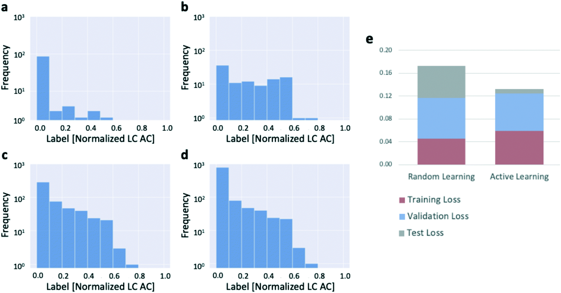Fig. 4 Results of active learning (ensemble-based uncertainty sampling) applied to the 3-bromopyridine data. (a)–(d): Log histograms of the outcomes of reactions added to the training dataset by the active learning algorithm show preferential selection of productive reactions. (a) 100 randomly-selected initialization reactions. (b) First 100 reactions selected by active learning. (c) First 500 reactions selected by active learning. (d) First 1000 reactions selected by active learning. (e) Distribution of total model loss across the training, validation, and test sets, for both random and active learning.

We expect that it will be possible to use active learning to drive test set error to extremely small values in any setting where a preponderance of the dataset labels have identical or nearly-identical values. To test this, we subsampled the Suzuki data to create augmented versions of the dataset with skewed, rather than uniform, label distributions. The results show performance intermediate between that of the 3-bromopyridine data and the non-augmented Suzuki data, which confirms the strong influence of the label distribution and any relationship that may exist between the label distribution and the average experimental error rate across the dataset (section S3e†).

To further gauge the influence of experimental error on active learning performance, we also studied the effect of adding noise to the datasets. Not only does added noise reduce the performance of the models overall, as we would expect, it also reduces the degree to which active learning outperforms random learning (Fig. S13†). We also studied the effect of removing the zero-yielding reactions from the 3-bromopyridine dataset, which naturally results in a dataset with higher average experimental error. The resulting active learning trajectory shows a decay in test set loss that is much more gradual than that in Fig. 3c (Fig. S12†).

Compared to the Suzuki data, the 3-bromopyridine data is more difficult to model accurately for two reasons: first, the 3-bromopyridine data covers a broader scope of substrates and reaction types with fewer data points. Unlike the Suzuki data, which explores the performance of a single coupling reaction under a variety of conditions, the 3-bromopyridine data examines many different kinds of reactions, making any given data point less informative to the other data points in the set than is the case for the Suzuki data (Fig. S1†). Second, the 3-bromopyridine dataset reports LC area counts rather than product yields, such that the model must learn to model the productivities of the various reactions as well as the response factors of each product in order to produce accurate predictions. Thus, the 3-bromopyridine dataset presents a more challenging modeling problem than the Suzuki dataset, leaving more room for active learning to outperform random learning on the 3-bromopyridine data.

Put another way, the Suzuki data is very easy to model, even with data points that are selected at random from the domain. The high degree of similarity between each of the reactions in the Suzuki dataset implies that much of the information needed to model one of the reactions in the dataset is useful for modeling many of the other reactions in the dataset as well.

Uncertainty estimation strategies

We studied the use of two different uncertainty estimation strategies: ensembles of neural networks (in which a series of models are trained using the same dataset, but with different weight initializations) and MC dropout masks. Fig. 5 shows the results of conducting uncertainty sampling-based active learning with these two techniques. When applied to the Suzuki data, ensembles perform better than MC dropout masks for n < 4500; the techniques perform similarly thereafter. The two techniques perform similarly to one another when applied to the 3-bromopyridine data. The domain dependence of the relative performance of uncertainty quantification strategies observed here is consistent with prior research.⁴⁹

Fig. 5 Comparison of uncertainty estimation strategies: ensembles versus Monte Carlo (MC) dropout. (a) and (b): Loss trajectories; each trajectory is the average of three runs of the corresponding algorithm; bands represent 95% confidence intervals. (a) 3-Bromopyridine data. (b) Suzuki data.

In order to understand the difference in the performance of the two techniques on the Suzuki data, we sought to evaluate the quality of the uncertainty estimates produced using both the ensembles approach and the MC dropout approach. Given that the predictions produced in both cases are normally distributed (Fig. S5†), if the uncertainty estimates are accurate or well-calibrated, the reported yield should fall within two standard deviations of the predicted mean roughly 95% of the time. One of the advantages of developing this strategy via a retrospective analysis is that we can readily evaluate whether this condition is satisfied without sacrificing any of our training data (Fig. S6 and S7†).

Although the MC dropout uncertainty estimation strategy performs slightly worse than ensembles, it is substantially less computationally expensive. Therefore, we sought to understand the influence of the number of dropout masks on the frequency with which the resulting standard deviation in the prediction effectively captured the distance between the prediction and the true yield, as well as its influence on the performance of active learning, with a specific interest in whether increasing the number of masks would allow us to meet or exceed the performance achieved with ensembles consisting of 100 members. We found that committees of ten masks yield better uncertainty estimates than committees of two masks, but increasing the number of masks further (to 100 and to 1000) does not further improve the quality of the estimates (Fig. S7†).

The greater accuracy of the uncertainty estimates produced when ten versus two dropout masks are used to estimate uncertainty does not translate to a meaningful difference in active learning performance (Fig. 6). This indicates that despite the magnitudes of the uncertainty estimates exhibiting varying degrees of “correctness,” the uncertainty estimation techniques rank the candidate reactions in similar orders.

Fig. 6 Influence of the number of dropout masks on the performance of active learning.

Influence of batch size

The number of experiments suggested by the algorithm in a single iteration without a degradation in performance compared to single-experiment batches is important to evaluate. It determines the number of experiments that can be performed in parallel, which is a critical feature of experiment planning and design. We expect performance to degrade with increasing batch size because there is a possibility of redundancy among the experiments that are recommended within a single iteration. Note that we do not mean to imply that increasing the size of the training dataset may inhibit performance, but merely that when comparing two training datasets of equal size, one generated with a large active learning batch size and one generated with a small active learning batch size, we expect the dataset generated with the smaller active learning batch size to have a lower test set error. To understand this, consider the following: if the model is highly uncertain about one reaction, it is reasonable to expect that the model is also highly uncertain about reactions that are similar to that one, yet it may not be necessary to add more than the first reaction to the training set to eliminate the bulk of the uncertainty.

Good performance is achieved across the range of batch sizes that were tested (Fig. 7). For the 3-bromopyridine data, although all four of the batch sizes tested achieve roughly the same final test set loss, the trajectory corresponding to a batch size of 384 does show degradation in performance compared to smaller batch sizes. Likewise, in the Suzuki data, when the training/validation dataset contains fewer than ∼2000 reactions, performance degrades by a small amount with increasing batch size. The four trajectories converge later on.

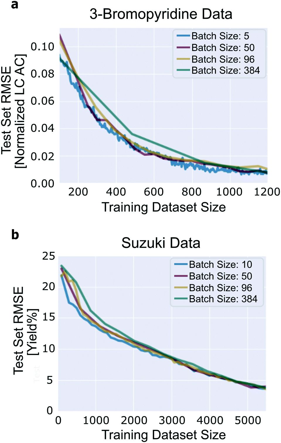Fig. 7 Influence of batch size. (a) 3-Bromopyridine data; (b) Suzuki data. Results generated using uncertainty estimation based on ensembles of neural networks with committee size 10.

When chemists implement this technique prospectively, the batch size parameter must be thoughtfully considered. The experimental convenience of large batch sizes must be balanced against the possibility for redundancy within those batches. Focusing on the generation of small batches of high-quality data accelerate convergence of the model. In the long run, this strategy will generally prove more efficient than executing larger batches of lower-quality experiments.

Conclusions

The presented results confirm that uncertainty sampling-based active learning is a useful experiment selection tool that can be helpfully applied in a variety of reaction domains, allowing medicinal and process chemists to focus their reaction screening efforts on the generation of a small amount of high-quality data. Furthermore, it is possible to propose large batches of experiments upon each iteration without a drastic reduction in performance, making it possible to perform the experiments recommended by the algorithm in a parallel fashion. Although a myriad of important factors contribute to the design of high-throughput reaction screening experiments, we recommend using this algorithm to navigate broad reaction domains, because models with broad domains of applicability are most useful long-term; the trade-off is that the accuracy may be lower compared to using the same quantity of experiments to train a model in a smaller domain.

Between the two different uncertainty estimation strategies that we evaluated (ensembles and MC dropout masks), ensembles delivered better active learning performance. However, the performance boost associated with ensembles needs to be balanced against the lower computational expense of the MC dropout approach. For datasets of sizes similar to those we work with here, computational expense is not a major concern, but this would change with larger datasets.

Our analysis suggests that the relatively large difference between random learning and uncertainty sampling observed for the 3-bromopyridine data is largely an artefact of the dataset's outcome distribution, and unproductive reactions exhibiting low experimental error. However, we also hypothesize that the general difficulty associated with modeling a particular dataset might also be a contributing factor to the amount by which active and random learning performance differs, since random learning can perform quite well for tasks where the individual data points have much in common and are highly informative to one another (as is the case for the Suzuki data).

The integration of this algorithm with a high-throughput reaction screening platform would facilitate better understanding of the myriad of factors that may contribute to the difference between active and random learning when operating on these kinds of datasets. Other factors of interest not discussed here include those related to the initialization of the algorithm, such as the number of reactions included in the initialization and the design of the initialization.

Conflicts of interest

There are no conflicts to declare.

Acknowledgements

We thank Pfizer for funding this research. We thank Xinjun Hou, Christopher Butler, and Qingyi Yang for helpful discussions. We thank Hanyu Gao for providing comments on the manuscript.

Notes and references

1. J. A. DiMasi, H. G. Grabowski and R. W. Hansen, J. Health Med. Econ., 2016, 20–33.
2. A. Buitrago-Santanilla, E. L. Regalado, T. Pereira, M. Shevlin, K. Bateman, L.-C. Campeau, J. Schneeweis, S. Berritt, Z.-C. Shi, P. Nantermet, Y. Liu, R. Helmy, C. J. Welch, P. Vachal, I. W. Davies, T. Cernak and S. D. Dreher, Science, 2015, 347, 6217.
3. D. Perera, J. W. Tucker, S. Brahmbhatt, C. J. Helal, A. Chong, W. Farrell, P. Richardson and N. W. Sach, Science, 2018, 359, 6374.
4. M. Wleklinski, B. P. Loren, C. R. Ferreira, Z. Jaman, L. Avramova, T. J. P. Sobreira, D. H. Thompson and R. G. Cooks, Chem. Sci., 2018, 9, 1647–1653.
5. D. W. Robbins and J. F. Hartwig, Science, 2011, 333(6048), 1423–1427.
6. X. W. Diefenbach, I. Farasat, E. D. Guetschow, C. J. Welch, R. T. Kennedy, S. Sun and J. C. Moore, ACS Omega, 2018, 3(2), 1498–1508.
7. M. T. Reetz, Angew. Chem., Int. Ed., 2001, 40(2), 284–310.
8. M. Shevlin, ACS Med. Chem. Lett., 2017, 8(6), 601–607.
9. P. M. Murray, S. N. G. Tyler and J. D. Moseley, Org. Process Res. Dev., 2013, 17, 40–46.
10. B. J. Reizman and K. F. Jensen, Acc. Chem. Res., 2016, 49(9), 1786–1796.
11. A. R. Bogdan and A. W. Dombrowski, J. Med. Chem., 2019, 62(14), 6422–6468.
12. C. Mateos, M. J. Nieves-Remacha and J. A. Rincón, React. Chem. Eng., 2019, 4(9), 1536–1544.
13. B. J. Reizman, Y.-M. Wang, S. L. Buchwald and K. F. Jensen, React. Chem. Eng., 2016, 1(6), 658–666.
14. L. M. Baumgartner, C. W. Coley, B. J. Reizman, K. W. Gao and K. F. Jensen, React. Chem. Eng., 2018, 3(3), 301–311.
15. S. Krishnadasan, R. J. C. Brown, A. J. DeMello and J. C. DeMello, Lab Chip, 2007, 7(11), 1434–1441.
16. J. E. Kreutz, A. Shukhaev, W. Du, S. Druskin, O. Daugulis and R. F. Ismagilov, J. Am. Chem. Soc., 2010, 132(9), 3128–3132.
17. F. Häse, L. M. Roch, C. Kreisbeck and A. Aspuru-Guzik, ACS Cent. Sci., 2018, 4(9), 1134–1145.
18. A.-C. Bédard, A. Adamo, K. C. Aroh, M. G. Russell, A. A. Bedermann, J. Torosian, B. Yue, K. F. Jensen and T. F. Jamison, Science, 2018, 361(6408), 1220–1225.
19. D. T. Ahneman, J. G. Estrada, S. Lin, S. D. Dreher and A. G. Doyle, Science, 2018, 360(6385), 186–190.
20. M. K. Nielsen, D. T. Ahneman, O. Riera and A. G. Doyle, J. Am. Chem. Soc., 2018, 140(15), 5004–5008.
21. B. Settles, Synthesis Lectures on Artificial Intelligence and Machine Learning, 2012, vol. 6, pp. 1–114.
22. Y. Fujiwara, Y. Yamashita, T. Osoda, M. Asogawa, C. Fukushima, M. Asao, H. Shimadzu, K. Nakao and R. Shimizu, J. Chem. Inf. Model., 2008, 48(4), 930–940.
23. M. K. Warmuth, J. Liao, G. Rätsch, M. Mathieson, S. Putta and C. Lemmen, J. Chem. Inf. Comput. Sci., 2003, 43(2), 667–673.
24. J. D. Kangas, A. W. Naik and R. F. Murphy, BMC Bioinf., 2014, 15, 143.
25. A. W. Naik, J. D. Kangas, D. P. Sullivan and R. F. Murphy, eLife, 2016, 5, e10047.
26. D. Reker, P. Schneider and G. Schneider, Chem. Sci., 2016, 7(6), 3919–3927.
27. K. de Grave, J. Ramon and L. de Raedt, International Conference on Discovery Science, 2008, pp. 185–196.
28. K. Williams, E. Bilsland, A. Sparkes, W. Aubrey, M. Young, L. N. Soldatova, K. de Grave, J. Ramon, M. de Clare, W. Sirawaraporn, S. G. Oliver and R. D. King, J. R. Soc., Interface, 2015, 12, 104.
29. O. Soufan, W. Ba-Alawi, M. Afeef, M. Essack, P. Kalnis and V. B. Bajic, J. Cheminf., 2016, 8, 64.
30. D. Reker and G. Schneider, Drug Discovery Today, 2015, 20(4), 458–465.
31. K. Tran and Z. W. Ulissi, Active learning across intermetallics to guide discovery of electrocatalysts for CO2 reduction and H2 evolution, Nat. Catal., 2018, 1(9), 696–703.
32. Y.-P. Li, K. Han, C. A. Grambow and W. H. Green, J. Phys. Chem. A, 2019, 123(10), 2142–2152.
33. J. S. Smith, B. T. Nebgen, R. Zubatyuk, N. Lubbers, C. Devereux, K. Barros, S. Tretiak, O. Isayev and A. E. Roitberg, Nat. Commun., 2019, 10, 2903.
34. E. V. Podryabinkin and A. V. Shapeev, Comput. Mater. Sci., 2017, 140, 171–180.
35. J. S. Smith, B. Nebgen, N. Lubbers, O. Isayev and A. E. Roitberg, J. Chem. Phys., 2018, 148, 241733.
36. K. Gubaev, E. V. Podryabinkin and A. V. Shapeev, J. Chem. Phys., 2018, 148, 241727.
37. R. D. King, K. E. Whelan, F. M. Jones, P. G. K. Reiser, C. H. Bryant, S. H. Muggleton, D. B. Kell and S. G. Oliver, Nature, 2004, 427(6971), 247–252.
38. A. A. Melnikov, H. P. Nautrup, M. Krenn, V. Dunjko, M. Tiersch, A. Zeilinger and H. J. Briegel, Proc. Natl. Acad. Sci. U. S. A., 2018, 115(6), 1221–1226.
39. D. A. Pertusi, M. E. Moura, J. G. Jeffryes, S. Prabhu, B. W. Biggs and K. E. J. Tyo, Metab. Eng., 2017, 44, 171–181.
40. D. D. Lewis and W. A. Gale, ACM SIGIR Forum, 1994, pp. 3–12.
41. A. Malinin and M. Gales, Conference on Neural Information Processing Systems, 2018, pp. 7047–7058.
42. B. Lakshminarayanan, A. Pritzel and C. Blundell, Conference on Neural Information Processing Systems, 2017, pp. 6402–6413.
43. G. Scalia, C. A. Grambow, B. Pernici, Y.-P. Li and W. H. Green, J. Chem. Inf. Model., 2020, 60(6), 2697–2717.
44. J. P. Janet, C. Duan, T. Yang, A. Nandy and H. J. Kulik, Chem. Sci., 2019, 10(34), 7913–7922.
45. Y. Gal and Z. Ghahramani, International Conference on Machine Learning, 2016, pp. 1050–1059.
46. D. Rogers and M. Hahn, J. Chem. Inf. Model., 2010, 50(5), 742–754.
47. G. Landrum, RDKit: Open-source cheminformatics, http://www.rdkit.org.
48. J. M. Granda, L. Donina, V. Dragone, D.-L. Long and L. Cronin, Nature, 2018, 559(7714), 377–381.
49. L. Hirschfeld, K. Swanson, K. Yang, R. Barzilay and C. W. Coley, 2020, arXiv:2005.10036.

---

Footnote

† Electronic supplementary information (ESI) available: Additional algorithm and dataset details, results, and discussion. See DOI: 10.1039/d0re00232a

---