
 Open Access Article
 This Open Access Article is licensed under a Creative Commons Attribution-Non Commercial 3.0 Unported Licence
Spin-state dependence of the structural and vibrational properties of solvated iron(II) polypyridyl complexes from AIMD simulations: III. [Fe(tpen)]Cl2 in acetonitrile†
Latévi M. Lawson Daku
Département de Chimie Physique, Université de Genève, Quai E. Ansermet 30, CH-1211 Genève 4, Switzerland. E-mail: max.lawson@unige.ch
First published on 7th December 2020
Abstract
In order to achieve an in-depth understanding of the role played by the solvent in the photoinduced low-spin (LS) → high-spin (HS) transition in solvated Fe(II) complexes, an accurate description of the solvated complexes in the two spin states is required. To this end, we are applying state-of-the-art ab initio molecular dynamics (AIMD) simulations to the study of the structural and vibrational properties of iron(II) polypyridyl complexes. Two aqueous LS complexes were investigated in this framework, namely, [Fe(bpy)3]2+ (bpy = 2,2′-bipyridine) [Lawson Daku and Hauser, J. Phys. Chem. Lett., 2010, 1, 1830; Lawson Daku, Phys. Chem. Chem. Phys., 2018, 20, 6236] and [Fe(tpy)2]2+ (tpy = 2,2′:6′,2′′-ter-pyridine) [Lawson Daku, Phys. Chem. Chem. Phys., 2019, 21, 650]. For aqueous [Fe(bpy)3]2+, combining the results of forefront wide-angle X-ray scattering experiments with those of the AIMD simulations allowed the visualization of the interlaced coordination and solvation spheres of the photoinduced HS state [Khakhulin et al., Phys. Chem. Chem. Phys., 2019, 21, 9277]. In this paper, we report the extension of our AIMD studies to the spin-crossover complex [Fe(tpen)]2+ (tpen = N,N,N′,N′-tetrakis(2-pyridylmethyl)ethylenediamine) in acetonitrile (ACN). The determined LS and HS solution structures of the complex are in excellent agreement with the experimental results obtained by high-resolution transient X-ray absorption spectroscopy [Zhang et al., ACS Omega, 2019, 4, 6375]. The first solvation shell of [Fe(tpen)]2+ consists of ACN molecules located in the grooves defined by the chelating coordination motif of the tpen ligand. Upon the LS → HS change of states, the solvation number of the complex is found to increase from ≈9.2 to ≈11.9 and an inner solvation shell is formed. This inner solvation shell originates from the occupancy by about one ACN molecule of the internal cavity which results from the arrangement of the 4 pyridine rings of the tpen ligand, and which becomes accessible to the solvent molecules in the HS state only thanks to the structural changes undergone by the complex. The presence of this inner solvation shell for the solvated HS complex probably plays a key role in the spin-state dependent reactivity of [Fe(tpen)]2+ in liquid solutions.
1 Introduction
The accurate description of transition metal complexes in liquid solutions is a challenging fundamental research problem, which must be tackled in order to achieve an in-depth understanding of the role played by the solvent in the photoinduced low-spin (LS) → high-spin (HS) transition in solvated hexacoordinated Fe(II) complexes. These complexes can indeed exhibit the phenomenon of spin crossover (SCO), that is the entropy-driven thermal depopulation of their ligand-field LS electronic ground state of octahedral 1A1(t2g6) parentage in favor of their ligand-field HS metastable state of octahedral 5T2(t2g4eg2) parentage.1 Light irradiation can also be used to induce the LS ⇄ HS change of states in both SCO and so-called LS complexes whose HS state lies too high in energy to be thermally populated.2–4 SCO complexes with a large energy barrier between the two states also show the phenomenon of light-induced excited spin-state trapping (LIESST), wherein the complexes become trapped in the HS state because the HS → LS relaxation following the photoinduced population of the HS state become too slow at low temperatures.3,4 The ability to use light irradiation to control the spin state of these complexes makes them ideal candidates for the studies of fundamental photophysical processes in transition metal complexes.5–7The mechanism of the photoinduced LS → HS change of states is thus being thoroughly investigated for SCO and LS Fe(II) polypyridyl complexes in solution using ultrafast vibrational,8–10 UV-vis,10–17 and X-ray18–40 spectroscopies. This way, new insights are being gained into the electronic state dynamics and into the structural dynamics of the FeIIN6 core, which includes the accurate determination of the changes in the Fe–N bond lengths. And, recently, advances in the understanding of the ultrafast photoinduced dynamics in a solvated [2 × 2] iron(II) metallogrid could be achieved by combining the three types of ultrafast spectroscopies.41 However, these ultrafast spectroscopy studies tend to leave open questions regarding the evolution of the whole molecular edifice, the influence of the solvent on the becoming of the photoexcited complex and the response of the solvation shell. Answering these questions requires an accurate description of the complexes in solution. To this end, we have undertaken a series of studies wherein we apply state-of-the-art ab initio molecular dynamics (AIMD) simulations to the study of the spin-state dependence of the structural and vibrational properties of solvated iron(II) polypyridyl complexes. We have studied the prototypical LS [Fe(bpy)3]2+ (bpy = 2,2′-bipyridine) complex in water.42,43 The results obtained have proved to constitute current reference data for classical MD studies44,45 and experimental data analysis.26,33–35 Actually, the combination of the AIMD simulations with forefront X-ray absorption spectroscopy (XAS) and wide-angle X-ray scattering (WAXS) experiments allowed the visualization of the interlaced coordination and solvation spheres of the aqueous [Fe(bpy)3]2+ in the photoinduced HS state.38 We have also investigated the aqueous LS [Fe(tpy)2]2+ (tpy = 2,2′:6′,2′′-ter-pyridine) complex.46 The comparison of the results similarly obtained for the chemically close LS complexes [Fe(tpy)2]2+ and [Fe(bpy)3]2+ allowed to probe the influence of the coordination motif (tetragonal versus trigonal) on their hydration structure. In this paper, we extend our AIMD studies to a SCO complex in acetonitrile (ACN), namely, [Fe(tpen)]2+ where tpen denotes the hexadentate N,N,N′,N′-tetrakis(2-pyridylmethyl)ethylenediamine ligand.47 With its distinct molecular architecture and the presence of inequivalent metal–ligand bonds, [Fe(tpen)]2+ is a very attractive transition metal system for fundamental photophysical studies; and, in this respect, the photoinduced LS → HS change of states has been investigated for [Fe(tpen)]2+ in ACN by high-resolution transient X-ray absorption spectroscopy (TXAS).37 Interestingly also, the racemization of the solvated complex is proposed to be coupled with the SCO equilibrium.48–51 Furthermore [Fe(tpen)]2+ exhibits in liquid solutions a spin-state dependent reactivity towards superoxide, dioxygen and nitric oxide,52–54 which remains to be fully understood. In terms of structure–properties relationships, this raises the question as to know which structural modifications entailed by the change of spin states can explain the spin-state dependence of these reactions. Consequently, with the present AIMD study of [Fe(tpen)]2+ in ACN, we aim at achieving an accurate description of the [Fe(tpen)]2+ solution in the LS and in the HS state, from which a first insight could also be gained into the origin of this spin-state dependent reactivity.
2 Computational details
The studied system consists of one [Fe(tpen)]2+ complex, 2 Cl− counterions and 109 acetonitrile molecules in a cubic box of side 23 Å (Fig. 1).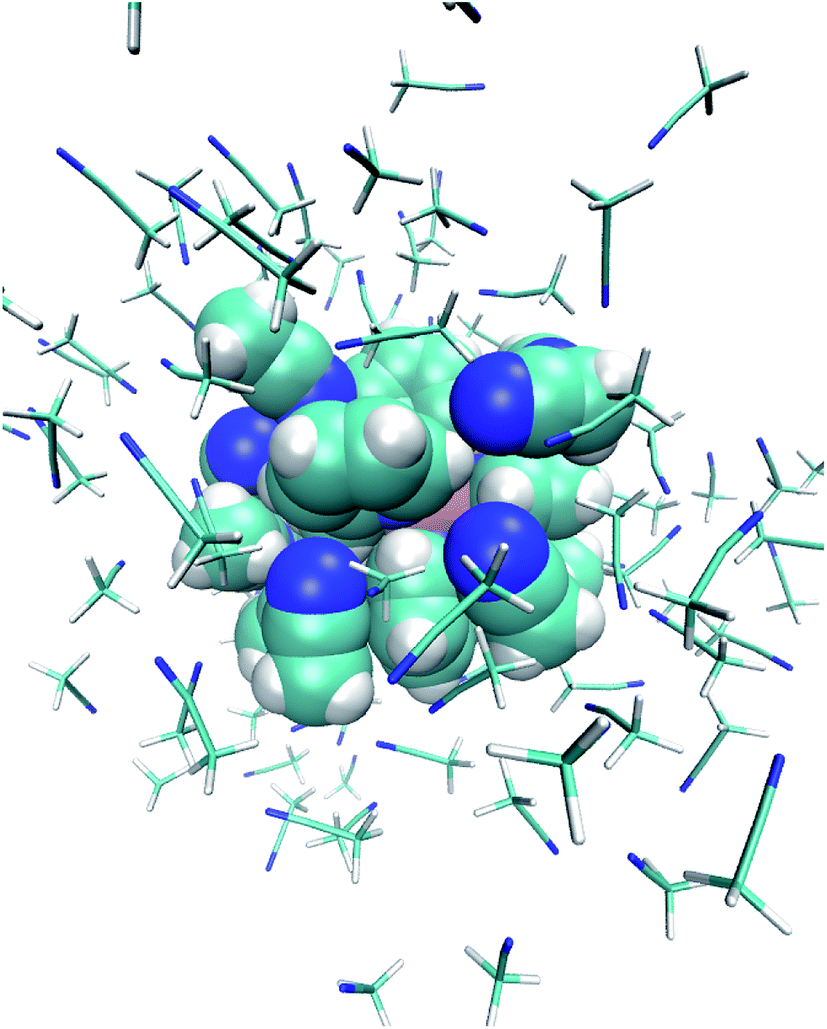 | ||
| Fig. 1 Snapshot from the HS trajectory (t = 6662.5 fs): [Fe(tpen)]2+ and the ACN molecules in its first solvation shell are drawn with a van der Waals representation, and the ACN molecules located beyond the first solvation shell with a licorice representation. | ||
2.1 Initial configurations
The initial LS configuration was obtained from a preliminary classical MD simulation of 1 ns duration followed by an optimization performed within DFT using the theoretical level described below. The classical MD simulation was run at 300 K with the GROMACS program package55,56 using the OPLS all-atom (OPLS-AA) force field for describing the Cl− ions and the ACN solvent molecules,57–62 and employing for the description of LS [Fe(tpen)]2+ kept fixed to its optimized geometry37 an approximate approximate model generated with the MKTOP program.63 The initial HS configuration was obtained from a DFT optimization performed in the HS state using a snapshot of the LS production trajectory as starting point.2.2 BOMD simulations
The settings are similar to those used in our previous BOMD studies.43,46 The simulations were thus performed with the dispersion-corrected BLYP-D3 functional64–66 and the hybrid Gaussian and planewave (GPW) method67 as implemented in the CP2K/QUICKSTEP program.68 The core electrons of the atoms were described with Goedecker–Teter–Hutter pseudopotentials,69–71 while their valence states were described with the Gaussian-type MOLOPT72 DZVP-MOLOPT-SR-GTH basis set of double-zeta polarized quality from the CP2K package. The electron density was expanded in a planewave basis set using a planewave cutoff of 800 Ry and a relative density cutoff of 50 Ry was used. The self-consistent-field calculations were run restricted for the LS state and unrestricted for the HS state. A timestep of 0.5 fs was employed for the integration of the equations of motion. Starting from the initial LS (resp., HS) configuration, the system was equilibrated in the LS (resp., HS) state for 10 ps at constant temperature (T = 310 K). The temperature was controlled by putting a Nosé–Hoover thermostat chain73 on each ionic degree of freedom (massive thermostating). Thermostating was kept on during the production runs, and the trajectories were recorded every 5 steps (i.e., every 2.5 fs). The lengths of the recorded LS and HS trajectories are ΘLS = 72.0825 ps and ΘHS = 69.0175 ps, respectively.2.3 Dipole moments and infrared spectra
For the calculations of the dipole moments of the constituents of the solution, the charge distribution was decomposed in terms of maximally-localized Wannier functions (MLWFs).74 Because of the significant computational cost of the localization procedure, the decomposition was done on the fly with the CP2K program68 every 10 steps (i.e., every 5.0 fs) only and for the last ΘWLS = 25.3275 ps (resp., ΘWHS = 26.2625 ps) of the simulation in the LS (resp., HS) state, during which the Wannier function centers (WFCs) were recorded. Denoting {riM}, the WFCs of a molecule M, its dipole moment reads
 | (1) |
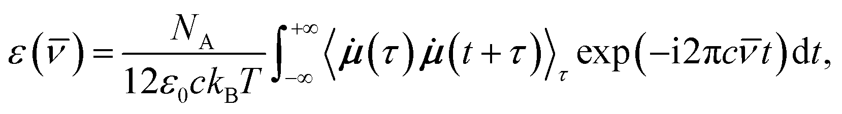 | (2) |
![[small nu, Greek, macron]](https://www.rsc.org/images/entities/i_char_e0ce.gif) is the wavenumber of the incident light, NA is the Avogadro number, c is the speed of light in vacuum, ε0 is the vacuum permittivity, kB is the Boltzmann constant, T is the average simulation temperature, i the imaginary unit, τ and t are time variables,
is the wavenumber of the incident light, NA is the Avogadro number, c is the speed of light in vacuum, ε0 is the vacuum permittivity, kB is the Boltzmann constant, T is the average simulation temperature, i the imaginary unit, τ and t are time variables, ![[small mu, Greek, dot above]](https://www.rsc.org/images/entities/b_i_char_e153.gif) is the time derivative of the dipole moment μ, and 〈(τ)(t + τ)〉τ is the autocorrelation function (ACF) of whose Fourier transform is actually taken. The WFC trajectories being recorded every 5 fs, the IR spectra were computed for wavenumbers up to νIRmax = 2500 cm−1.
is the time derivative of the dipole moment μ, and 〈(τ)(t + τ)〉τ is the autocorrelation function (ACF) of whose Fourier transform is actually taken. The WFC trajectories being recorded every 5 fs, the IR spectra were computed for wavenumbers up to νIRmax = 2500 cm−1.
2.4 Additional analyses and visualization
The average LS and HS solution structures of [Fe(tpen)]2+ and the distribution functions of selected structural parameters were calculated using utilities from the GROMACS program package.55,56 Radial distributions functions and associated running coordination numbers were computed with the Travis program,75,76,78 which was also used for the calculations of spatial distribution functions and combined distribution functions. Molecular visualizations were created with the VMD79,80 and the Jmol81–83 programs. Curves were plotted using the Matplotlib program package.843 Results and discussion
3.1 Structural properties
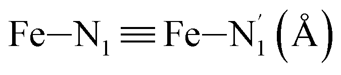
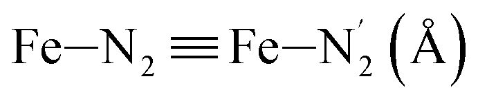
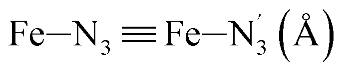
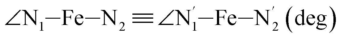
 ; the length of the bonds between the Fe and the pyridyl N (Npyridyl) atoms
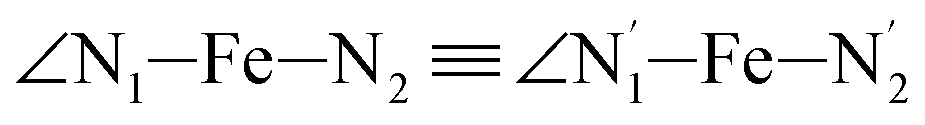
  , the fitting plane to the Ni and
  atoms (i = 1, 2) defining the equatorial plane of an idealized tetragonal coordination sphere; the bonds between the Fe and the axial Npyridyl atoms
  ; and the Fe–N bond angles
  ,
,  ,
,  , and
, and  (see Fig. 2 for the atom labeling used). From the experimental point of view, the recent high-resolution TXAS study by Canton et al.37 allowed to distinguish between the Fe–N bonds involving the Naminyl atoms (N1 and
  ) and those involving the Npyridyl atoms (Ni and
  with i = 2, 3). However such a distinction could not be made between these latter ones. Hence, to allow a direct comparison with the experimental results, we have also calculated the distribution of the length of the bonds between the Fe and the four Npyridyl atoms, thereafter also denoted Nα.
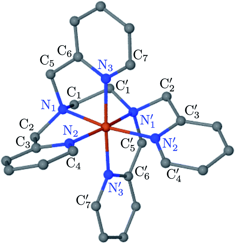 | ||
Fig. 2 Average solution structure of LS [Fe(tpen)]2+ of C1 symmetry showing the atom labeling used. In the ideal C2 symmetry, the atoms Xi and  (X = N and i = {1, 2, 3}, or X = C and i = {1, …, 7}) are interchanged by the C2 operation. (X = N and i = {1, 2, 3}, or X = C and i = {1, …, 7}) are interchanged by the C2 operation. | ||
The distributions of the Fe–N bond lengths are plotted in Fig. 3. They are quite broad for [Fe(tpen)]2+ in the LS state, which reflects the large thermal fluctuations undergone by the solvated complex. They become broader and exhibit a ∼0.2 Å shift towards longer bond lengths for HS [Fe(tpen)]2+, as a consequence of the weakening of the Fe–N bonds and the accompanying increase in the thermal fluctuations. The LS → HS change of states indeed involves the promotion of two electrons from the mostly nonbonding metallic Fe(3d) orbitals of octahedral t2g parentage into the antibonding metallic Fe(3d) orbitals of octahedral eg parentage. One also notes that in either spin state, the distributions of the  and
and  bonds lengths strongly overlap. This explains why it proves difficult to discriminate experimentally between the two types of Fe–Npyridyl bond lengths.37
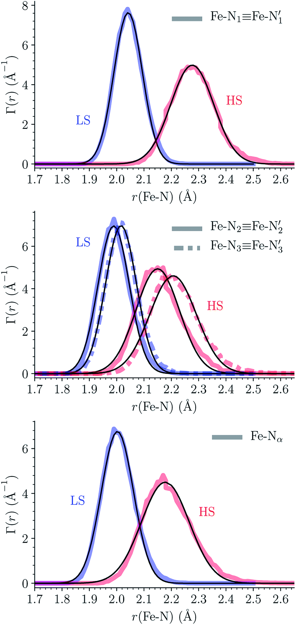 | ||
Fig. 3 Distribution functions of the Fe–N bond lengths for [Fe(tpen)]2+ in acetonitrile and in the LS and HS states (thick solid or dashed lines). Nα designates the pyridyl nitrogen atoms Ni and  . The fits of the data with Gaussians are also shown (black lines). . The fits of the data with Gaussians are also shown (black lines). | ||
The distributions of the selected Fe–N bond angles are plotted in Fig. 4. As observed for the distribution of the Fe–N bond lengths, these distributions are broad for LS [Fe(tpen)]2+ and become broader for HS [Fe(tpen)]2+ because of the increased thermal fluctuations accompanying the weakening of the Fe–N bonds. For LS [Fe(tpen)]2+, the  angle distribution function is strongly asymmetric: it is peaked around 178 deg, smoothly decreasing towards smaller angle values while abruptly vanishing towards higher values. This is due to the chelating coordination motif of the tpen hexadentate ligand which prevents this angle from taking values higher than 178 deg. Note that, although it is less pronounced, the asymmetry of the
  angle distribution is maintained for HS [Fe(tpen)]2+. Upon the LS → HS change of states, the
  ,
,  and
and  angles decrease by ∼5 deg to ∼7 deg while the
 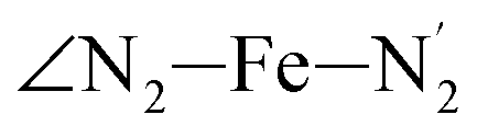 angle increases by ∼17 deg: this reflects the rearrangement of the tpen ligand around the Fe atom entailed by the lengthening of the Fe–N bonds.
 | ||
Fig. 4 Distribution functions of the ∠N–Fe–N angles for [Fe(tpen)]2+ in acetonitrile and in the LS and HS (thick solid lines). The fits of the data are also shown (black lines): all data were fitted with Gaussians except for the  angle whose distributions were fitted with skewed Gaussians. angle whose distributions were fitted with skewed Gaussians. | ||
The Fe–N distances distributions could be satisfactorily fitted using Gaussian distributions functions (Fig. 3). They exhibit a slight departure from an ideal Gaussian distribution, which is more marked for [Fe(tpen)]2+ in the HS state. These slight deviations from Gaussian distributions can be ascribed to the anharmonicity of the motion of the complex on its free energy surface, especially along the Fe–N distance coordinates.43,46 The distributions of the ∠N–Fe–N angles could all be well fitted with Gaussian distributions, except those of the  angle for which skewed Gaussian distributions were used so as to take into account the asymmetry of its distributions (Fig. 4).
Table 1 summarizes the averages and standard deviations obtained from the fits of the Fe–N bond lengths. The 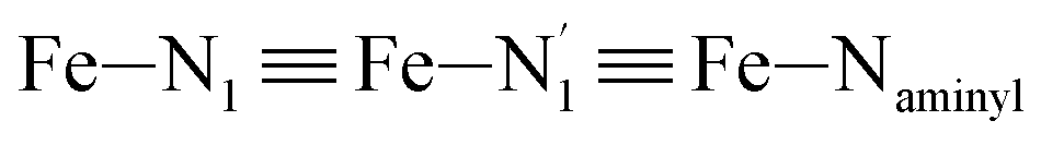 bond lengths are predicted to increase from 2.042 Å to 2.277 Å on going from the LS to the HS state, and the Fe–Nα
![[triple bond, length as m-dash]](https://www.rsc.org/images/entities/char_e002.gif) Fe–Npyridyl bond lengths are predicted to increase from 2.003 Å to 2.178 Å. These results are in excellent agreement with the experimental ones85 also reported in Table 1. This attests for the high accuracy of the structural information gained from the AIMD simulations. This is the case for the distinction achieved between the axial and equatorial Fe–Npyridyl bond lengths: the LS to HS change of states is thus found to be accompanied by the increase of the
Fe–Npyridyl bond lengths are predicted to increase from 2.003 Å to 2.178 Å. These results are in excellent agreement with the experimental ones85 also reported in Table 1. This attests for the high accuracy of the structural information gained from the AIMD simulations. This is the case for the distinction achieved between the axial and equatorial Fe–Npyridyl bond lengths: the LS to HS change of states is thus found to be accompanied by the increase of the  bond length from 1.989 Å to 2.150 Å and of the
 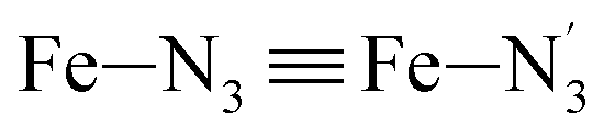 bond length from 2.016 Å to 2.206 Å. Consequently, the Fe–Naminyl bonds show the largest lengthening (+0.235 Å) upon the LS → HS transition, followed by the axial Fe–Npyridyl bonds (+0.190 Å) and then by equatorial Fe–Npyridyl bonds (+0.161 Å).
![[X with combining macron]](https://www.rsc.org/images/entities/i_char_0058_0304.gif) ) and standard deviations (σ(X)) of selected structural parameters characterizing the LS and HS solution structures of [Fe(tpen)]2+ in acetonitrile: results of the fit of the parameter distributions using Gaussian distribution functions, except for the
) and standard deviations (σ(X)) of selected structural parameters characterizing the LS and HS solution structures of [Fe(tpen)]2+ in acetonitrile: results of the fit of the parameter distributions using Gaussian distribution functions, except for the 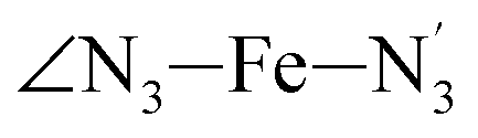 angle whose distributions were fitted with skewed Gaussian distribution functions (see Text). λ is the skewness parameter entering the definition of the skewed Gaussian distributions. Available experimental data are also showna
| AIMD | Exp. | |||||
|---|---|---|---|---|---|---|
|
σ(X) | λ | In ACNb | |||
a Nα designates the pyridyl nitrogen atoms Ni and  ; Π1 is the angle between the three-atom planes ; Π1 is the angle between the three-atom planes  and and  respectively defined by the basis vectors respectively defined by the basis vectors  and and  , and Π2 is the angle between the three-atom planes , and Π2 is the angle between the three-atom planes  and and  .defined by the basis vectors .defined by the basis vectors  and and  , respectively.b Ref. 37. , respectively.b Ref. 37. |
||||||
 |
LS | 2.042 | 0.052 | 2.02(2) | ||
| HS | 2.277 | 0.078 | 2.26(2) | |||
 |
LS | 1.989 | 0.057 | — | ||
| HS | 2.150 | 0.079 | — | |||
 |
LS | 2.016 | 0.057 | — | ||
| HS | 2.206 | 0.085 | — | |||
| Fe–Nα (Å) | LS | 2.003 | 0.059 | 1.98(2) | ||
| HS | 2.178 | 0.088 | 2.15(2) | |||
 |
LS | 87.4 | 2.3 | |||
| HS | 79.8 | 3.0 | ||||
 |
LS | 109.4 | 3.1 | |||
| HS | 127.4 | 5.0 | ||||
 |
LS | 81.8 | 2.3 | |||
| HS | 77.1 | 3.1 | ||||
 |
LS | 178.4 | 3.8 | −3.2 | ||
| HS | 173.6 | 5.8 | −1.1 | |||
| Π1 (deg) | LS | 88.9 | 6.7 | |||
| HS | 93.7 | 8.3 | ||||
| Π2 (deg) | LS | 144.7 | 7.3 | |||
| HS | 150.6 | 11.4 | ||||
Table 1 also summarizes the averages and standard deviations obtained from the fits of the selected ∠N–Fe–N angles. For the  angle whose distributions in the LS and HS states have been fitted with skewed Gaussian distribution functions, the values found for the skewness parameter λ are also reported: λ < 0 as expected for left-skewed distributions and its magnitude decreases from 3.2 to 1.1 on going from the LS to the HS state as a consequence of the reduced asymmetry of the distribution.
The angle Π1 between the three-atom planes  and
and  and the angle Π2 between the three-atom planes
  and
and  have been introduced to describe the relative orientations of the axial pyridine rings and of the equatorial ones, respectively. Their LS and HS distributions could be satisfactorily fitted with Gaussian distribution functions, as shown in the ESI (Fig. S1†). The averages and standard deviations obtained from the fits for Π1 and Π2 are given in Table 1. Π1 is found to increase from 88.9 deg to 93.7 deg on passing from the LS to the HS state, and Π2 from 144.7 deg to 150.6 deg. That is, the axial pyridine rings thus tend to remain perpendicular in the two spin states and the twist between the equatorial pyridine rings decreases on passing from the LS to the HS state.
In order to characterize further the arrangement of tpen around the Fe atom beyond the FeN6 first coordination sphere, the distributions of the  bond lengths have been calculated as well as those of the Fe–Cβ, Fe–Cγ and Fe–Cδ bond lengths, which, in addition to the
  bond length, could be experimentally determined for [Fe(tpen)]2+ in ACN.37 Here, Cβ designates the ligand's chemically equivalent C atoms Ci and
  (i = 3, 6), Cγ the atoms Ci and
  (i = 2, 5), and Cδ the atoms Ci and
  (i = 4, 7). These distributions have been satisfactorily fitted with Gaussian functions (Fig. S2 and S3, ESI†). The averages and standard values of the Fe–C bond lengths thus obtained are summarized in Table 2 along with the available experimental data, with which a good agreement is also observed.
) and standard deviations (σ(X)) of selected Fe–C distances characterizing the LS and HS solution structures of [Fe(tpen)]2+ in acetonitrile: results of the fit of the parameter distributions using Gaussians. Available experimental data are also showna
| AIMD | Exp. | |||
|---|---|---|---|---|
|
σ(X) | In ACNb | ||
a Cβ designates the carbon atoms Ci and  (i = 3, 6), Cγ the carbon atoms Ci and (i = 3, 6), Cγ the carbon atoms Ci and  (i = 2, 5), and Cδ the atoms Ci and (i = 2, 5), and Cδ the atoms Ci and  (i = 4, 7).b Ref. 37. (i = 4, 7).b Ref. 37. |
||||
 |
LS | 2.845 | 0.057 | 2.82(3) |
| HS | 3.071 | 0.093 | 2.98(2) | |
 |
LS | 2.826 | 0.054 | |
| HS | 2.999 | 0.086 | ||
 |
LS | 2.820 | 0.053 | |
| HS | 2.981 | 0.078 | ||
 |
LS | 3.022 | 0.073 | |
| HS | 3.132 | 0.105 | ||
 |
LS | 2.944 | 0.059 | |
| HS | 3.113 | 0.094 | ||
 |
LS | 2.878 | 0.053 | |
| HS | 3.045 | 0.088 | ||
 |
LS | 3.022 | 0.072 | |
| HS | 3.183 | 0.102 | ||
| Fe–Cβ (Å) | LS | 2.850 | 0.062 | 2.87(3) |
| HS | 3.011 | 0.090 | 3.04(2) | |
| Fe–Cγ (Å) | LS | 2.886 | 0.090 | 2.93(3) |
| HS | 3.056 | 0.110 | 3.10(2) | |
| Fe–Cδ (Å) | LS | 3.022 | 0.073 | 3.03(3) |
| HS | 3.158 | 0.107 | 3.20(2) | |
The LS and HS average solution structures of [Fe(tpen)]2+ have been calculated and stereoscopic views of them are shown in Fig. 5 and 6, respectively. The 50% probability ellipsoids associated with the thermal fluctuations of the atoms about their average positions are also represented. The inspection of each figure shows that, in either spin state, the thermal fluctuations increase on moving away from the metal atom and hence with the exposure of the atoms to the solvent, the smallest atomic displacements being for the atoms which belong to five-membered chelate rings. The comparison of the two figures shows that the LS → HS change of states is accompanied by an increase of the atomic disorder as measured by the volumes of the ellipsoids.
 | ||
| Fig. 5 Stereoscopic view of the average structures of LS [Fe(tpen)]2+ in acetonitrile with the 50% probability ellipsoids. | ||
 | ||
| Fig. 6 Stereoscopic view of the average structures of HS [Fe(tpen)]2+ in acetonitrile with the 50% probability ellipsoids. | ||
The thermal ellipsoids of the atoms of the tpen ligand are strongly anisotropic. Such a privileged directionality of the atomic displacements can be explained by the strength and directionality of the Fe–N bonds and also by the rigidity of the hexadentate tpen ligand, be it the rigidity of pyridyl moities or the one which results from its chelating coordination motif. For the atoms belonging to the pyridine rings of tpen, the major principal axes of their thermal ellipsoids tend to be perpendicular to the average planes of the rigid pyridine rings: this follows from the rigidity of the rings and from the strong and directional character of the Fe–N bonds which hinder the atomic motion along directions parallel to the average planes of the pyridine rings.46 As for the CH2 groups of tpen, the major principal axes of the thermal ellipsoids associated with the atomic displacements tend to be located in the planes defined by the average positions of their atoms. This can be ascribed to the fact that the out-of-plane motions of their atoms are hindered by the belonging of their C atoms to five-membered chelate rings whose conformational flexibility is somehow limited by the requirement to maintain the Fe(II)-tpen bonding optimal.
C1ACN–C2ACN) and hydrogen (HACN) atoms with respect to the Fe atom. They are plotted in Fig. 7 along with the associated running coordinations numbers.
 | ||
| Fig. 7 Solvation structure of [Fe(tpen)]2+ in the LS (top) and in the HS state (bottom): radial distribution functions g(r) of the acetonitrile nitrogen (NACN), carbon (NACNC1ACN–C2ACN) and hydrogen (HACN) atoms with respect to the Fe atom (solid lines, left y-axis), and running coordination numbers cn(r) (dashed lines, left y-axis). | ||
LS [Fe(tpen)]2+. For [Fe(tpen)]2+ in the LS state, the Fe–NACN, Fe–C1ACN and Fe–C2ACN RDFs exhibit each a first well-resolved peak at ≈5.6 Å, ≈6.1 Å and ≈6.7 Å, respectively, with a minimum at ≈6.6 Å, ≈7.3 Å and ≈7.7 Å, respectively. The presence and ordering of these peaks indicates that the first solvation shell of LS [Fe(tpen)]2+ is structured, and that the ACN molecules present in this solvation shell tend to be oriented with their NACN heads pointing toward the Fe atom. The fact that the 0.5–0.6 Å distance between the peaks does not match the interactomic distances in the ACN molecule suggests that there is no colinearity between (i) the line passing through the Fe atom and the NACN atom of the observed ACN molecule and (ii) the ACN molecular axis simply taken as the one defined by its nitrile group. This is supported by the plot in Fig. 8 of the combined r(Fe–NACN)/ϕ radial/angular distribution function (CDF): ϕ is the angle ∠FeNACNC1ACN where NACN and C1ACN are the atoms of the nitrile group belonging to the ACN molecule observed at a distance r from the Fe atom. For the ACN molecules in the first solvation shell (r(Fe–NACN) ≤ 6.6 Å), one indeed notes in Fig. 8 that the r(Fe–NACN)/ϕ CDF exhibits a broad and tall peak culminating at r ≈ 5.6 Å ϕ ≈ 100 deg and covering the area delimited by 5.0 Å ≤ r ≤ 6.1 Å and 90 deg ≲ ϕ ≲ 120 deg. Besides these dominantly preferred orientations, ACN molecules in the first solvation shell adopt orientations with ϕ > 120 deg. For 6.6 Å ≲ r ≲ 8.5 Å, that is, for ACN molecules in the second solvation shell (see below), the preferred orientations correspond to 70 deg ≤ ϕ ≤ 180 deg. One also observes a massif covering the area delimited by 8.6 Å ≤ r ≤ 10.0 Å and 0 deg ≲ ϕ ≲ 40 deg. Beyond r = 10 Å, in the bulk, no real preferential ϕ orientation is observed.
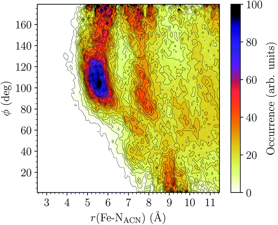 | ||
| Fig. 8 Combined r(Fe–NACN)/ϕ radial/angular distribution function for [Fe(tpen)]2+ in the LS state; ϕ is the angle ∠FeNACNC1ACN where NACN and C1ACN are the atoms of the nitrile group belonging to the ACN molecule observed at a distance r from the Fe atom. | ||
One notes in Fig. 7 that the Fe–NACN and Fe–C1ACN RDFs present a second peak at ≈7.7 Å and ≈8.1 Å, respectively, with a minimum at ∼8.7 Å for both RDFs. These features indicate the presence of a second solvation shell, which, however, is not as structured as the first solvation shell in that the Fe–C2ACN RDF does not exhibit a well-defined second peak. The Fe–HACN RDF shows a main broad peak at ≈7.3 Å with a shallow minimum at ∼9.3 Å. It takes non-vanishing values at distances shorter than the other RDFs because the ACN H atoms can go closer to the Fe atom than the ACN N and C atoms of larger van der Waals radii. The number of ACN molecules in the first solvation shell of LS [Fe(tpen)]2+, namely its solvation number, is given by the value of the Fe–NACN running coordination number at the position of the minimum associated with the first peak of the Fe–NACN RDF. It thus amounts to ≈9.2. As illustrated by the snapshot from the HS trajectory (Fig. 1), the ACN molecules of the first solvation enter the grooves defined by the coordinating tpen ligand.
HS [Fe(tpen)]2+. Upon the LS → HS change of states, the Fe–NACN, Fe–C1ACN and Fe–C2ACN RDFs are shifted to lower distances (Fig. 7): that is, the lengthening of the Fe–N bonds and the accompanying structural rearrangement of the tpen ligand allow the ACN molecules to go closer to the Fe atom. The Fe–NACN and Fe–C1ACN RDFs present also a peak at ≈4.4 Å and ≈4.5 Å, respectively, with a minimum at ≈4.7 Å and ≈5.1 Å, respectively, while the Fe–CC2ACN RDF shows a shoulder centered at ≈5.0 Å. This indicates the formation of an inner solvation shell with ≈0.8 ACN molecule. The main peaks of the Fe–NACN, Fe–C1ACN and Fe–C2ACN are broader than in the LS state with their maxima displaced to longer distances at ≈6.1 Å, ≈6.6 Å and ≈7.4 Å, respectively, and their minima at ≈7.1 Å, ≈7.6 Å and ≈9.8 Å, respectively. The broad peak of the Fe–HACN RDF is also displaced to longer distance, at ≈8.0 Å, with its shallow minimum moved to ≈9.5 Å. Thus, on passing from the LS to the HS state, the first solvation shell of [Fe(tpen)]2+ becomes less structured. Fig. 9 shows the plot of the r(Fe–NACN)/ϕ CDF calculated for the complex in the HS state. The peak at r ≈ 4.2 Å shows that the ≈0.8 ACN molecule entering the inner solvation shell adopts orientations distributed around ϕ ≈ 100 deg, while the massif located at r ≈ 6.0 Å indicates preferred orientations centered about ϕ ≈ 120 deg for the other ACN molecules in the first solvation shell. The solvation number of HS [Fe(tpen)]2+ is ≈11.9. It follows that about 3 ACN molecules enter the first solvation shell of [Fe(tpen)]2+ upon the LS → HS change of states.
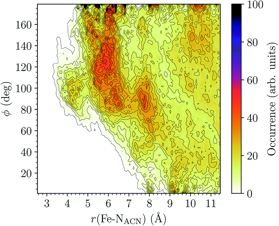 | ||
| Fig. 9 Combined r(Fe–NACN)/ϕ radial/angular distribution function for [Fe(tpen)]2+ in the HS state; ϕ is the angle ∠FeNACNC1ACN where NACN and C1ACN are the atoms of the nitrile group belonging to the ACN molecule observed at a distance r from the Fe atom. | ||
The inner solvation shell of HS [Fe(tpen)]2+ has been characterized by calculating the spatial distribution function (SDF) of the NACN atom belonging to the ACN molecule(s) entering the inner shell. These are the ACN molecules for which r(Fe–NACN) ≤ 4.7 Å (Fig. S4, ESI†). A stereoscopic view of the SDF is shown in Fig. 10 along with its contour plot in the plane defined by the N3 and Fe atoms and by the barycenter of the N2 and  atoms. The inspection of the SDF shows that the ACN molecule in the inner solvation shell is dominantly located in the internal cavity which results from the arrangement of the 4 pyridine rings. The internal cavity can be schematically depicted as the polyhedral cone whose generators pass through the Fe atom and the four H atoms, Hi and
  , which are respectively attached to the Ci and
  (i = 4, 7) of the pyridine rings. The ACN molecule can be located on either side of the equatorial plane defined by the fitting plane to the Ni and
  atoms (i = 1, 2). The cavity is not accessible to the solvent molecules in the LS state, its entrance being hindered by the Hi and
  (i = 4, 7) atoms. Upon the LS → HS change of states, it becomes accessible since these H atoms move away as a results of the lengthening of the Fe–N bonds and to the concomitant large widening of the
  bond angle, as anticipated in ref. 37. The fact that this internal cavity can become accessible to molecules as small as ACN in the HS state only probably explains why [Fe(tpen)]2+ exhibits a spin-state dependent reactivity towards dioxygen, superoxide or nitric oxide.52–54 We will elaborate on the entailment of our finding for the chemical reactivity of the complex in the “Conclusion and outlook” Section, after having completed the AIMD characterization of the [Fe(tpen)]2+ solution.
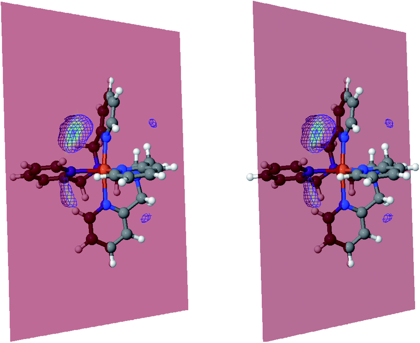 | ||
Fig. 10 Stereoscopic view of the spatial distribution function of the NACN atoms of the ACN molecules entering the inner solvation shell of HS [Fe(tpen)]2+: the meshed isosurface corresponds to a particule density of 30 nm−3 (density range: 0 to 552 nm−3), and the contour plot is in the plane defined by the N3 and Fe atoms and by the barycenter of the N2 and  atoms (see Fig. 2 for the atom labeling scheme). atoms (see Fig. 2 for the atom labeling scheme). | ||
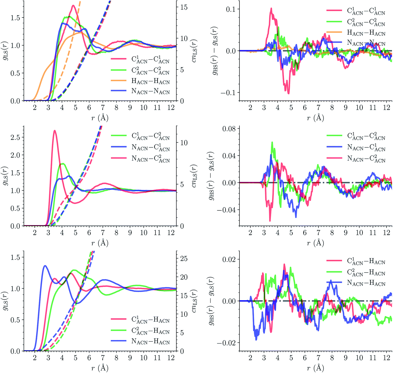 | ||
| Fig. 11 Structure of the acetonitrile solvent state (atom labeling: NACNC1ACN–C2ACN(HACN)3): (left) intermolecular radial distribution functions g(r) (solid lines, left y-axis) and running coordination numbers cn(r) (dashed lines, left y-axis) for [Fe(tpen)]2+ in the LS state; (right) differences between the HS and LS radial distribution functions. | ||
The solvation structure of the Cl− anions has been characterized in the two spin states by calculating the Cl–X (X = HACN, NACN, C1ACN, C2ACN) RDFs. Fig. 12 shows the plot of the LS Cl–X RDFs with the associated running coordination numbers, as well as the plot of the differences gHS(r) − gLS(r) between the HS and LS Cl–X RDFs. The relatively small magnitudes of the difference curves indicate a weak dependence of the solvation structure of the anions on the spin state of [Fe(tpen)]2+. Longer simulation times would allow for a decrease of the noise in the RDFs and hence for a better signal-to-noise ratio of the gHS(r) − gLS(r) curves whose magnitudes would probably also decrease. The Cl–HACN, Cl–C2ACN and Cl–C1ACN RDFs show well-resolved peaks at ≈2.6 Å, ≈3.5 Å, ≈4.2 Å, respectively, which all three lead to a coordination number of ≈6 (see also Fig. S7, ESI†). That is, for the complex in either spin state, the first solvation shell of Cl− is very structured and made of 6 H-bonded ACN molecules. Two snapshots from the LS trajectory illustrating the first solvation shell of the Cl− anions are presented in Fig. S8 (ESI†). During the AIMD simulations, the Cl− counteranions are found to stay in the vicinity of the [Fe(tpen)]2+ complex in either spin state (Fig. S9, ESI†), which can be ascribed to the moderately dissociating power of the ACN solvent. The formation of such associations between the large [Fe(tpen)]2+ complex and the Cl− anions for this 0.136 M [Fe(tpen)]Cl2 solution probably explains why the present solvation number of Cl− of 6 is significantly smaller than the one of 9.5 determined by Fischer et al. for the anion in ACN at infinite dilution from Monte Carlo simulations.88
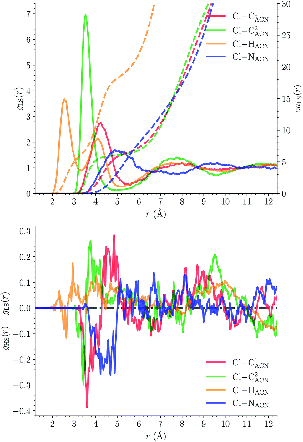 | ||
| Fig. 12 Solvation structure of Cl− in acetonitrile (atom labeling: NACNC1ACN–C2ACN(HACN)3): (top) radial distribution functions g(r) (solid lines, left y-axis) and running coordination numbers cn(r) (dashed lines, left y-axis) for [Fe(tpen)]2+ in the LS state; (bottom) differences between the HS and LS radial distribution functions. | ||
3.2 Dipole moments
The dipole distribution functions (DDFs) determined for [Fe(tpen)]2+ in the two spin states are plotted in Fig. 13. The DDF calculated for LS [Fe(tpen)]2+ is quite broad, the magnitude of the instantaneous dipole moment varying between 1 D and 7 D. The DDF is broader and shifted towards smaller values for HS [Fe(tpen)]2+, the instantaneous dipole moment ranging from 0 D to 7 D. The dipole moments deduced from these DDFs for the solvated complex in the LS and in the HS state are 4.26 ± 0.99 D and 3.61 ± 1.07 D, respectively.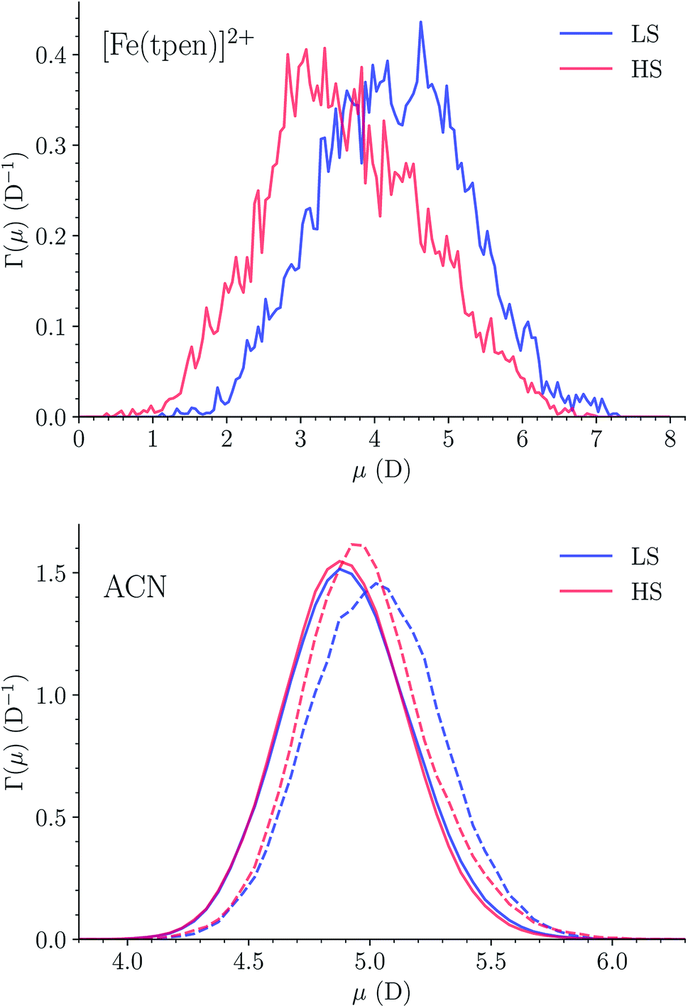 | ||
| Fig. 13 Dipole distribution functions of (top) [Fe(tpen)]2+ in the LS and in the HS state, and of (bottom) the ACN molecules in (r(Fe–NACN) ≤ r1,min, dashed lines) and beyond (r(Fe–NACN) > r1,min, solid lines) the first solvation shell of [Fe(tpen)]2+ in the LS and in the HS state (r1,min|LS = 6.6 Å, r1,min|HS = 7.1 Å). | ||
The DDFs of the solvent molecules in and beyond the first solvation shell of [Fe(tpen)]2+ have also been determined. They are plotted in Fig. 13. The DDFs obtained for the ACN molecules in the bulk do not depend on the spin state of [Fe(tpen)]2+. They lead to a molecular dipole moment of 4.90 ± 0.26 D, which is in good agreement with the experimental value of 4.5 ± 0.1 D determined for liquid ACN by Ohba and Ikawa.89 The DDFs obtained for the ACN molecule in the first solvation shell of [Fe(tpen)]2+ are slightly shifted towards larger values, the shift being larger in the LS state than in the HS state. This reflects the spin-state dependence of the polarization of the solvation shell, which translates into dipole moments of 5.02 ± 0.27 D and 4.98 ± 0.27 D for the ACN molecules in the first solvation shell of [Fe(tpen)]2+ in the LS and HS states, respectively.
3.3 Vibrational properties
Fig. 14 shows the calculated LS and HS 310 K IR spectra of [Fe(tpen)]2+ in ACN. They have similar shapes and the intensity of the IR absorption bands tends to be stronger in the HS state than in the LS state, as illustrated by the plot of the HS-LS difference spectrum which could be use as a reference in transient IR absorption spectroscopy studies. The absorption peak present in the LS and HS spectra at 2290 cm−1 is reminiscent of the intense ν2 CN stretching absorption band of ACN located at this same wavenumber (Fig. S10†). Its contribution to the spectra cancels out in the HS-LS difference spectrum.
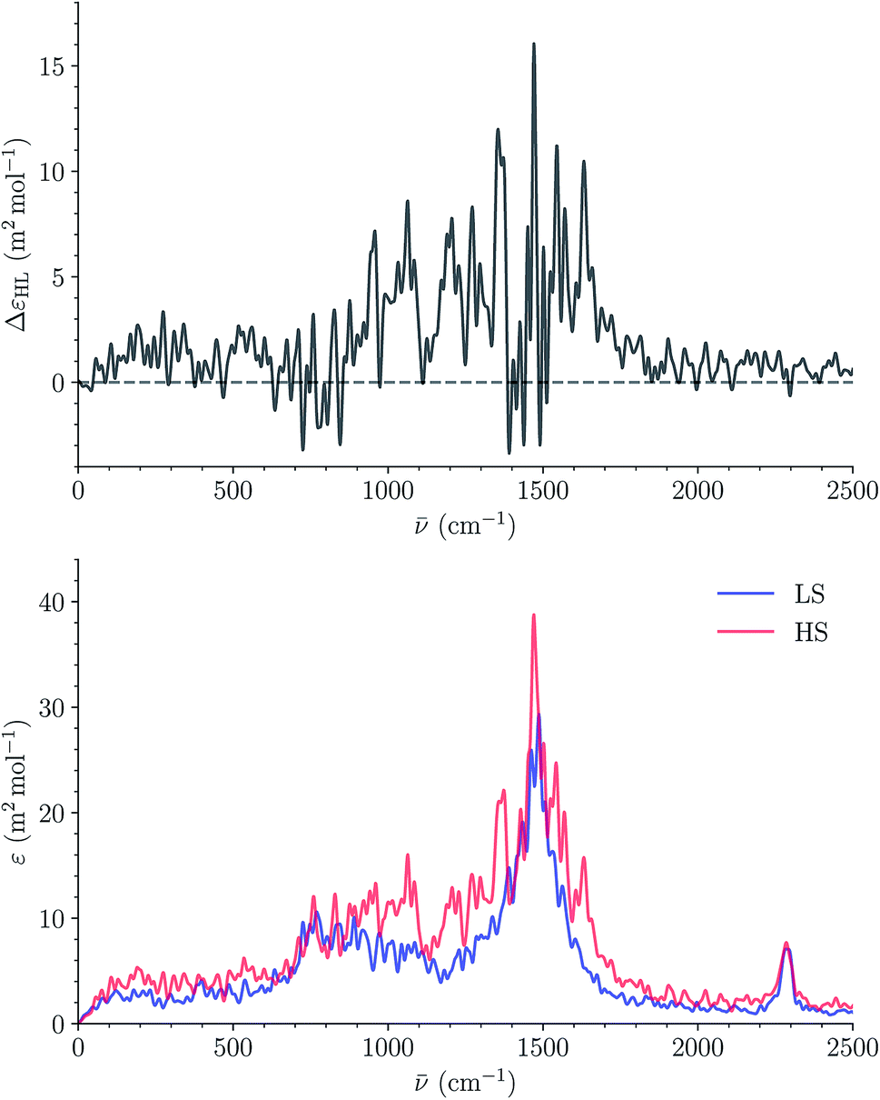 | ||
| Fig. 14 Calculated LS and HS 310 K IR spectra of [Fe(tpen)]2+ in ACN (bottom) and corresponding HS-LS difference curve (top; resolution of the ACFs: 512 time steps). | ||
4 Conclusion and outlook
The present AIMD study allowed us to achieve a detailed characterization of the [Fe(tpen)]2+ SCO complex in ACN. The determination of its solution structure in the LS and in the HS state gave results in excellent agreement with those recently obtained by high-resolution TXAS.37 Insights could be gained into the solvation structure of the complex and its spin-state dependence. Thus, the first solvation shell of [Fe(tpen)]2+ consists of ACN molecules located in the grooves defined by the chelating coordination motif of the tpen ligand. Furthermore, upon the LS to HS change of states, the solvation number of [Fe(tpen)]2+ increases from ≈9.2 to ≈11.9 and an inner solvation shell is formed. The LS and HS IR spectra of [Fe(tpen)]2+ have been calculated and the AIMD approach used for the calculation allowed to directly take into account thermal, anharmonic and vibrational effects.90–94 The two spectra show similar shapes, with an increase of the intensity of the absorption bands on going from the LS to the HS state. This same feature was observed for the LS and HS spectra similarly calculated for [Fe(bpy)3]2+ and [Fe(tpy)2]2+ in water.43,46The three solvated complexes have also in common that their atomic disorder depends on their spin state and on the exposure of the observed atoms to the solvent. More generally, their thermal fluctuation turns out to be stronger the weaker the metal–ligand bonds, whose strength and directionality, in conjunction with the rigidity of the coordinating ligands, seem to dictate the directionality of the atomic displacements. A strong interpenetration between the coordination sphere and the solvation shell is observed for the three complexes as well. For [Fe(tpen)]2+ in ACN, the entanglement is such that an inner solvation shell is formed on passing from the LS to the HS state. About one ACN molecule is associated with this inner solvation shell and it is located in the internal cavity which results from the arrangement of the 4 pyridine rings. This cavity becomes accessible in the HS state only thanks the structural changes undergone by [Fe(tpen)]2+ upon the LS → HS change of state. The inner shell corresponds to the presence of an ACN molecule in the close vicinity of the Fe(II) ion with its NACN head directed towards the Fe(II) ion, a situation which thereafter can lead to the formation of a bond between the ACN molecule and the Fe(II) ion, that is, to its heptacoordination. The racemization of [Fe(tpen)]2+ and of other chiral SCO Fe(II) complexes is proposed to be coupled with the SCO equilibrium.48–51 The identification of the inner solvation shell of HS [Fe(tpen)]2+ suggests that the enantiomerization of the complex in the HS state could be significantly assisted by the solvent.
In their electrochemical study of the activation of O2 by [Fe(tpen)]2+ under reductive conditions, Ségaud et al.54 have found that the reaction starts with the formation of a complex between [Fe(tpen)]2+ and O2. On the basis of the present results, it is likely that this [Fe(tpen)]2+–O2 complex results from the occupancy of the internal cavity of HS [Fe(tpen)]2+ by the dioxygen molecule. Interestingly also, Roncaroli and Meier investigated the kinetics of the reaction NO with [Fe(tpen)]2+ and also with a SCO and a LS derivative of [Fe(tpen)]2+.53 Quantitative reactions leading to the formation of a complex with NO were observed for the SCO complexes only, and for [Fe(tpen)]2+, the formation of the HS nitrosylated [Fe(tpen)NO]2+ was evidenced by EPR spectroscopy. The reactions were found to exhibit a second-order kinetics and the authors proposed a mechanism wherein the reaction proceeds through the displacement of a water solvent molecule in the HS heptacoordinated [Fe(tpen)OH2]2+ species.53 The finding of the inner solvation shell of HS [Fe(tpen)]2+ advocates for this mechanism. From there, it appears that the extension of the present AIMD study to the one in the LS and HS states of the enantiomerization of [Fe(tpen)]2+ in ACN and of its reaction with dioxygen, nitric oxide or superoxide52 would provide valuable insights into the spin-state dependence of the reactivity of [Fe(tpen)]2+ and its derivatives in solution.
Conflicts of interest
There are no conflicts to declare.Acknowledgements
This work was supported by grants from the Swiss National Supercomputing Centre (CSCS) under projects ID s501 and s894, and from the Center for Advanced Modeling Science (CADMOS) under Project ID CTESIM. LMLD thanks Sophie Canton and Hans Hagemann for fruitful discussions.References
- Spin Crossover in Transition Metal Compounds I-III, ed. P. Gütlich and H. A. Goodwin, Springer-Verlag, Heidelberg, 2004, vol. 233–235 Search PubMed.
- J. J. McGarvey and I. Lawthers, J. Chem. Soc., Chem. Commun., 1982, 906–907 RSC.
- S. Decurtins, P. Gütlich, C. P. Köhler, H. Spiering and A. Hauser, Chem. Phys. Lett., 1984, 105, 1–4 CrossRef CAS.
- A. Hauser, Top. Curr. Chem., 2004, 234, 155–198 CrossRef CAS.
- A. Hauser and C. Reber, Struct. Bonding, 2016, 172, 291–312 CrossRef.
- C. Daniel, Coord. Chem. Rev., 2015, 282–283, 19–32 CrossRef CAS.
- T. J. Penfold, E. Gindensperger, C. Daniel and C. M. Marian, Chem. Rev., 2018, 118, 6975–7025 CrossRef CAS.
- C. Brady, P. L. Callaghan, Z. Ciunik, C. G. Coates, A. Døssing, A. Hazell, J. J. McGarvey, S. Schenker, H. Toftlund, A. X. Trautwein, H. Winkler and J. A. Wolny, Inorg. Chem., 2004, 43, 4289–4299 CrossRef CAS.
- M. M. N. Wolf, C. S. R. Groß, J. A. Wolny, V. Schünemann, A. Døssing, H. Paulsen, J. J. McGarvey and R. Diller, Phys. Chem. Chem. Phys., 2008, 10, 4264–4273 RSC.
- A. L. Smeigh, M. Creelman, R. A. Mathies and J. K. McCusker, J. Am. Chem. Soc., 2008, 130, 14105–14107 CrossRef CAS.
- J. E. Monat and J. K. McCusker, J. Am. Chem. Soc., 2000, 122, 4092–4097 CrossRef CAS.
- W. Gawelda, A. Cannizzo, V.-T. Pham, F. van Mourik, C. Bressler and M. Chergui, J. Am. Chem. Soc., 2007, 129, 8199–8206 CrossRef CAS.
- A. Lapini, P. Foggi, L. Bussotti, R. Righini and A. Dei, Inorg. Chim. Acta, 2008, 361, 3937–3943 CrossRef CAS.
- C. Consani, M. Prémont-Schwarz, A. ElNahhas, C. Bressler, F. van Mourik, A. Cannizzo and M. Chergui, Angew. Chem., Int. Ed., 2009, 48, 7184–7187 CrossRef CAS.
- G. Auböck and M. Chergui, Nat. Chem., 2015, 7, 629–633 CrossRef.
- A. Moguilevski, M. Wilke, G. Grell, S. I. Bokarev, S. G. Aziz, N. Engel, A. A. Raheem, O. Kühn, I. Y. Kiyan and E. F. Aziz, ChemPhysChem, 2016, 18, 465–469 CrossRef.
- A. Ould Hamouda, F. Dutin, J. Degert, M. Tondusson, A. Naim, P. Rosa and E. Freysz, J. Phys. Chem. Lett., 2019, 10, 5975–5982 CrossRef CAS.
- M. Khalil, M. A. Marcus, A. L. Smeigh, J. K. McCusker, H. H. W. Chong and R. W. Schoenlein, J. Phys. Chem. A, 2006, 110, 38–44 CrossRef CAS.
- W. Gawelda, V.-T. Pham, M. Benfatto, Y. Zaushitsyn, M. Kaiser, D. Grolimund, S. L. Johnson, R. Abela, A. Hauser, C. Bressler and M. Chergui, Phys. Rev. Lett., 2007, 98, 057401 CrossRef.
- W. Gawelda, V.-T. Pham, R. M. van der Veen, D. Grolimund, R. Abela, M. Chergui and C. Bressler, J. Chem. Phys., 2009, 130, 124520 CrossRef CAS.
- C. Bressler, C. Milne, V.-T. Pham, A. ElNahhas, R. M. van der Veen, W. Gawelda, S. Johnson, P. Beaud, D. Grolimund, M. Kaiser, C. N. Borca, G. Ingold, R. Abela and M. Chergui, Science, 2009, 323, 489–492 CrossRef CAS.
- G. Vankó, P. Glatzel, V.-T. Pham, R. Abela, D. Grolimund, C. N. Borca, S. L. Johnson, C. J. Milne and C. Bressler, Angew. Chem., Int. Ed., 2010, 49, 5910–5912 CrossRef.
- S. Nozawa, T. Sato, M. Chollet, K. Ichiyanagi, A. Tomita, H. Fujii, S. ichi Adachi and S. ya Koshihara, J. Am. Chem. Soc., 2010, 132, 61–63 CrossRef CAS.
- N. Huse, T. K. Kim, L. Jamula, J. K. McCusker, F. M. F. de Groot and R. W. Schoenlein, J. Am. Chem. Soc., 2010, 132, 6809–6816 CrossRef CAS.
- N. Huse, H. Cho, K. Hong, L. Jamula, F. M. F. de Groot, T. K. Kim, J. K. McCusker and R. W. Schoenlein, J. Phys. Chem. Lett., 2011, 2, 880–884 CrossRef CAS.
- K. Haldrup, G. Vankó, W. Gawelda, A. Galler, G. Doumy, A. M. March, E. P. Kanter, A. Bordage, A. Dohn, T. B. van Driel, K. S. Kjær, H. T. Lemke, S. E. Canton, J. Uhlig, V. Sundström, L. Young, S. H. Southworth, M. M. Nielsen and C. Bressler, J. Phys. Chem. A, 2012, 116, 9878–9887 CrossRef CAS.
- H. T. Lemke, C. Bressler, L. X. Chen, D. M. Fritz, K. J. Gaffney, A. Galler, W. Gawelda, K. Haldrup, R. W. Hartsock, H. Ihee, J. Kim, K. H. Kim, J. H. Lee, M. M. Nielsen, A. B. Stickrath, W. Zhang, D. Zhu and M. Cammarata, J. Phys. Chem. A, 2013, 117, 735–740 CrossRef CAS.
- S. E. Canton, X. Zhang, L. M. Lawson Daku, A. L. Smeigh, J. Zhang, Y. Liu, C.-J. Wallentin, K. Attenkofer, G. Jennings, C. A. Kurtz, D. Gosztola, K. Wärnmark, A. Hauser and V. Sundström, J. Phys. Chem. C, 2014, 118, 4536–4545 CrossRef CAS.
- W. Zhang, R. Alonso-Mori, U. Bergmann, C. Bressler, M. Chollet, A. Galler, W. Gawelda, R. G. Hadt, R. W. Hartsock, T. Kroll, K. S. Kjaer, K. Kubicek, H. T. Lemke, H. W. Liang, D. A. Meyer, M. M. Nielsen, C. Purser, J. S. Robinson, E. I. Solomon, Z. Sun, D. Sokaras, T. B. van Driel, G. Vanko, T.-C. Weng, D. Zhu and K. J. Gaffney, Nature, 2014, 509, 345–348 CrossRef CAS.
- X. Zhang, M. L. Lawson Daku, J. Zhang, K. Suarez-Alcantara, G. Jennings, C. A. Kurtz and S. E. Canton, J. Phys. Chem. C, 2015, 119, 3312–3321 CrossRef CAS.
- S. E. Canton, X. Zhang, M. L. Lawson Daku, Y. Liu, J. Zhang and S. Alvarez, J. Phys. Chem. C, 2015, 119, 3322–3330 CrossRef CAS.
- G. Vankó, A. Bordage, M. Pápai, K. Haldrup, P. Glatzel, A. M. March, G. Doumy, A. Britz, A. Galler, T. Assefa, D. Cabaret, A. Juhin, T. B. van Driel, K. S. Kjær, A. Dohn, K. B. Møller, H. T. Lemke, E. Gallo, M. Rovezzi, Z. Németh, E. Rozsályi, T. Rozgonyi, J. Uhlig, V. Sundström, M. M. Nielsen, L. Young, S. H. Southworth, C. Bressler and W. Gawelda, J. Phys. Chem. C, 2015, 119, 5888–5902 CrossRef.
- K. Haldrup, W. Gawelda, R. Abela, R. Alonso-Mori, U. Bergmann, A. Bordage, M. Cammarata, S. E. Canton, A. O. Dohn, T. B. van Driel, D. M. Fritz, A. Galler, P. Glatzel, T. Harlang, K. S. Kjær, H. T. Lemke, K. B. Møller, Z. Németh, M. Pápai, N. Sas, J. Uhlig, D. Zhu, G. Vankó, V. Sundström, M. M. Nielsen and C. Bressler, J. Phys. Chem. B, 2016, 120, 1158–1168 CrossRef CAS.
- B. E. Van Kuiken, H. Cho, K. Hong, M. Khalil, R. W. Schoenlein, T. K. Kim and N. Huse, J. Phys. Chem. Lett., 2016, 7, 465–470 CrossRef CAS.
- H. T. Lemke, K. S. Kjær, R. Hartsock, T. B. van Driel, M. Chollet, J. M. Glownia, S. Song, D. Zhu, E. Pace, S. F. Matar, M. M. Nielsen, M. Benfatto, K. J. Gaffney, E. Collet and M. Cammarata, Nat. Commun., 2017, 8, 15342 CrossRef CAS.
- C. Liu, J. Zhang, L. M. Lawson Daku, D. Gosztola, S. E. Canton and X. Zhang, J. Am. Chem. Soc., 2017, 139, 17518–17524 CrossRef CAS.
- J. Zhang, X. Zhang, K. Suarez-Alcantara, G. Jennings, C. A. Kurtz, L. M. Lawson Daku and S. E. Canton, ACS Omega, 2019, 4, 6375–6381 CrossRef CAS.
- D. Khakhulin, L. M. Lawson Daku, D. Leshchev, G. E. Newby, M. Jarenmark, C. Bressler, M. Wulff and S. E. Canton, Phys. Chem. Chem. Phys., 2019, 21, 9277–9284 RSC.
- K. S. Kjær, T. B. Van Driel, T. C. B. Harlang, K. Kunnus, E. Biasin, K. Ledbetter, R. W. Hartsock, M. E. Reinhard, S. Koroidov, L. Li, M. G. Laursen, F. B. Hansen, P. Vester, M. Christensen, K. Haldrup, M. M. Nielsen, A. O. Dohn, M. I. Pápai, K. B. Møller, P. Chabera, Y. Liu, H. Tatsuno, C. Timm, M. Jarenmark, J. Uhlig, V. Sundstöm, K. Wärnmark, P. Persson, Z. Németh, D. S. Szemes, É. Bajnóczi, G. Vankó, R. Alonso-Mori, J. M. Glownia, S. Nelson, M. Sikorski, D. Sokaras, S. E. Canton, H. T. Lemke and K. J. Gaffney, Chem. Sci., 2019, 10, 5749–5760 RSC.
- A. Britz, W. Gawelda, T. A. Assefa, L. L. Jamula, J. T. Yarranton, A. Galler, D. Khakhulin, M. Diez, M. Harder, G. Doumy, A. M. March, É. Bajnóczi, Z. Németh, M. Pápai, E. Rozsályi, D. Sárosiné Szemes, H. Cho, S. Mukherjee, C. Liu, T. K. Kim, R. W. Schoenlein, S. H. Southworth, L. Young, E. Jakubikova, N. Huse, G. Vankó, C. Bressler and J. K. McCusker, Inorg. Chem., 2019, 58, 9341–9350 CrossRef CAS.
- M. A. Naumova, A. Kalinko, J. W. L. Wong, S. Alvarez Gutierrez, J. Meng, M. Liang, M. Abdellah, H. Geng, W. Lin, K. Kubicek, M. Biednov, F. Lima, A. Galler, P. Zalden, S. Checchia, P.-A. Mante, J. Zimara, D. Schwarzer, S. Demeshko, V. Murzin, D. Gosztola, M. Jarenmark, J. Zhang, M. Bauer, M. L. Lawson Daku, D. Khakhulin, W. Gawelda, C. Bressler, F. Meyer, K. Zheng and S. E. Canton, J. Chem. Phys., 2020, 152, 214301 CrossRef CAS.
- L. M. Lawson Daku and A. Hauser, J. Phys. Chem. Lett., 2010, 1, 1830–1835 CrossRef CAS.
- L. M. Lawson Daku, Phys. Chem. Chem. Phys., 2018, 20, 6236–6253 RSC.
- A. K. Das, R. V. Solomon, F. Hofmann and M. Meuwly, J. Phys. Chem. B, 2016, 120, 206–216 CrossRef CAS.
- S. Iuchi, J. Chem. Phys., 2012, 136, 064519 CrossRef.
- L. M. Lawson Daku, Phys. Chem. Chem. Phys., 2019, 21, 650–661 RSC.
- H. R. Chang, J. K. McCusker, H. Toftlund, S. R. Wilson, A. X. Trautwein, H. Winkler and D. N. Hendrickson, J. Am. Chem. Soc., 1990, 112, 6814–6827 CrossRef CAS.
- K. F. Purcell, J. Am. Chem. Soc., 1979, 101, 5147–5152 CrossRef CAS.
- L. G. Vanquickenborne and K. Pierloot, Inorg. Chem., 1981, 20, 3673–3677 CrossRef CAS.
- J. J. McGarvey, I. Lawthers, K. Heremans and H. Toftlund, Inorg. Chem., 1990, 29, 252–256 CrossRef CAS.
- J. K. McCusker, A. L. Rheingold and D. N. Hendrickson, Inorg. Chem., 1996, 35, 2100–2112 CrossRef CAS.
- M. Tamura, Y. Urano, K. Kikuchi, T. Higuchi, M. Hirobe and T. Nagano, Chem. Pharm. Bull., 2000, 48, 1514–1518 CrossRef CAS.
- F. Roncaroli and R. Meier, J. Coord. Chem., 2015, 68, 2990–3002 CrossRef CAS.
- N. Ségaud, E. Anxolabéhère-Mallart, K. Sénéchal-David, L. Acosta-Rueda, M. Robert and F. Banse, Chem. Sci., 2015, 6, 639–647 RSC.
- M. J. Abraham, T. Murtola, R. Schulz, S. Páll, J. C. Smith, B. Hess and E. Lindahl, SoftwareX, 2015, 1–2, 19–25 CrossRef.
- B. Hess, C. Kutzner, D. van der Spoel and E. Lindahl, J. Chem. Theory Comput., 2008, 4, 435–447 CrossRef CAS.
- W. L. Jorgensen, D. S. Maxwell and J. Tirado-Rives, J. Am. Chem. Soc., 1996, 118, 11225–11236 CrossRef CAS.
- W. L. Jorgensen and N. A. McDonald, J. Mol. Struct.: THEOCHEM, 1998, 424, 145–155 CrossRef CAS.
- W. L. Jorgensen and N. A. McDonald, J. Phys. Chem. B, 1998, 102, 8049–8059 CrossRef.
- R. C. Rizzo and W. L. Jorgensen, J. Am. Chem. Soc., 1999, 121, 4827–4836 CrossRef CAS.
- C. Caleman, P. J. van Maaren, M. Hong, J. S. Hub, L. T. Costa and D. van der Spoel, J. Chem. Theory Comput., 2012, 8, 61–74 CrossRef CAS.
- D. van der Spoel, P. J. van Maaren and C. Caleman, Bioinformatics, 2012, 28, 752–753 CrossRef CAS.
- A. Ribeiro, B. Horta and R. de Alencastro, J. Braz. Chem. Soc., 2008, 19, 1433–1435 CrossRef CAS.
- A. D. Becke, Phys. Rev. A: At., Mol., Opt. Phys., 1988, 38, 3098–3100 CrossRef CAS.
- C. Lee, W. Yang and R. G. Parr, Phys. Rev. B: Condens. Matter Mater. Phys., 1988, 37, 785–789 CrossRef CAS.
- S. Grimme, J. Antony, S. Ehrlich and H. Krieg, J. Chem. Phys., 2010, 132, 154104 CrossRef.
- G. Lippert, J. Hutter and M. Parrinello, Mol. Phys., 1997, 92, 477–487 CrossRef CAS.
- J. VandeVondele, M. Krack, M. Fawzi, M. Parrinello, T. Chassaing and J. Hutter, Comput. Phys. Commun., 2005, 167, 103–128 CrossRef CAS.
- S. Goedecker, M. Teter and J. Hutter, Phys. Rev. B: Condens. Matter Mater. Phys., 1996, 54, 1703–1710 CrossRef CAS.
- C. Hartwigsen, S. Goedecker and J. Hutter, Phys. Rev. B: Condens. Matter Mater. Phys., 1998, 58, 3641–3662 CrossRef CAS.
- M. Krack, Theor. Chem. Acc., 2005, 114, 145–152 Search PubMed.
- J. VandeVondele and J. Hutter, J. Chem. Phys., 2007, 127, 114105 CrossRef.
- G. J. Martyna, M. L. Klein and M. Tuckerman, J. Chem. Phys., 1992, 97, 2635–2643 CrossRef.
- N. Marzari, A. A. Mostofi, J. R. Yates, I. Souza, I. Souza and D. Vanderbilt, Rev. Mod. Phys., 2012, 85, 1419–1475 CrossRef.
- M. Brehm and B. Kirchner, J. Chem. Inf. Model., 2011, 51, 2007–2023 CrossRef CAS.
- M. Brehm, M. Thomas, S. Gehrke and B. Kirchner, J. Chem. Phys., 2020, 152, 164105 CrossRef CAS.
- M. Thomas, M. Brehm and B. Kirchner, Phys. Chem. Chem. Phys., 2015, 17, 3207–3213 RSC.
- K. A. F. Röhrig and T. D. Kühne, Phys. Rev. E: Stat., Nonlinear, Soft Matter Phys., 2013, 87, 045301 CrossRef.
- W. Humphrey, A. Dalke and K. Schulten, J. Mol. Graphics, 1996, 14, 33–38 CrossRef CAS.
- J. Stone, MSc thesis, Computer Science Department, University of Missouri-Rolla, 1998.
- Jmol: an open-source Java viewer for chemical structures in 3D, http://www.jmol.org, accessed November 2, 2017 Search PubMed.
- B. McMahon and R. M. Hanson, J. Appl. Crystallogr., 2008, 41, 811–814 CrossRef CAS.
- R. M. Hanson, J. Prilusky, Z. Renjian, T. Nakane and J. L. Sussman, Isr. J. Chem., 2013, 53, 207–216 CrossRef CAS.
- J. D. Hunter, Comput. Sci. Eng., 2007, 9, 90–95 Search PubMed.
- A. Hauser, C. Enachescu, M. Lawson Daku, A. Vargas and N. Amstutz, Coord. Chem. Rev., 2006, 250, 1642–1652 CrossRef CAS.
- S. Pothoczki and L. Pusztai, J. Mol. Liq., 2017, 225, 160–166 CrossRef CAS.
- J. Hernández-Cobos, J. M. Martínez, R. R. Pappalardo, I. Ortega-Blake and E. Sánchez Marcos, J. Mol. Liq., 2020, 318, 113975 CrossRef.
- R. Fischer, J. Richardi, P. H. Fries and H. Krienke, J. Chem. Phys., 2002, 117, 8467–8478 CrossRef CAS.
- T. Ohba and S. Ikawa, Mol. Phys., 1991, 73, 985–997 CrossRef CAS.
- A. J. R. da Silva, J. W. Pang, E. A. Carter and D. Neuhauser, J. Phys. Chem. A, 1998, 102, 881–885 CrossRef CAS.
- R. Ramírez, T. López-Ciudad, P. Kumar P and D. Marx, J. Chem. Phys., 2004, 121, 3973–3983 CrossRef.
- M.-P. Gaigeot, J. Phys. Chem. A, 2008, 112, 13507–13517 CrossRef CAS.
- M. Kaledin, J. M. Moffitt, C. R. Clark and F. Rizvi, J. Chem. Theory Comput., 2009, 5, 1328–1336 CrossRef CAS.
- S. D. Ivanov, A. Witt and D. Marx, Phys. Chem. Chem. Phys., 2013, 15, 10270–10299 RSC.
Footnote |
† Electronic supplementary information (ESI) available: Distribution functions of the angles Π1 and Π2. Distribution functions of the  distances. Distribution functions of the Fe–Cζ (ζ = β, γ, δ) distances. Snapshots from the HS trajectory showing ACN molecules in the inner solvation shell of HS [Fe(tpen)]2+. Radial distribution functions characterizing the structure of the acetonitrile solvent for [Fe(tpen)]2+ in the LS and HS states. Snapshots from the LS trajectory illustrating the first solvation shell of the Cl− counterions. Time dependence of the Fe–Cl distances for [Fe(tpen)]2+ in the LS and HS states. IR spectrum of the ACN solvent. Comparison between the IR spectra of [Fe(tpen)]Cl2 and [Fe(tpen)]2+ in ACN. See DOI: 10.1039/d0ra09499d distances. Distribution functions of the Fe–Cζ (ζ = β, γ, δ) distances. Snapshots from the HS trajectory showing ACN molecules in the inner solvation shell of HS [Fe(tpen)]2+. Radial distribution functions characterizing the structure of the acetonitrile solvent for [Fe(tpen)]2+ in the LS and HS states. Snapshots from the LS trajectory illustrating the first solvation shell of the Cl− counterions. Time dependence of the Fe–Cl distances for [Fe(tpen)]2+ in the LS and HS states. IR spectrum of the ACN solvent. Comparison between the IR spectra of [Fe(tpen)]Cl2 and [Fe(tpen)]2+ in ACN. See DOI: 10.1039/d0ra09499d |
| This journal is © The Royal Society of Chemistry 2020 |