
 Open Access Article
 This Open Access Article is licensed under a Creative Commons Attribution-Non Commercial 3.0 Unported Licence
First-principles investigation on the bonding mechanisms of two-dimensional carbon materials on the transition metals surfaces
Xin Zhang *ab,
Shenghui Sunab and
Shaoqing Wangb
*ab,
Shenghui Sunab and
Shaoqing Wangb
aShenyang National Laboratory for Materials Science, Institute of Metal Research, Chinese Academy of Sciences, 110016 Shenyang, Liaoning, China. E-mail: xzhang17b@imr.ac.cn
bSchool of Materials Science and Engineering, University of Science and Technology of China, 110016 Shenyang, Liaoning, China
First published on 9th December 2020
Abstract
Understanding the bonding mechanisms between carbon and metal atoms are crucial for experimental preparations of low-dimensional carbon materials and metal/low-dimensional carbon composites. In this work, various bonding modes are summarized through a systematical study on the adsorptions of graphene and graphyne on surfaces of typical transition metals. If a carbon atom is adjacent to a transition metal atom, the C-pz electron may form a covalent bond with a s or a d electron of the transition metal atom. When a metal atom lies below two carbon atoms of graphene or graphyne, two new covalent bonds may be formed between the metal atom and the two carbon atoms by two C-pz electrons with two d or two sd-hybridized orbital electrons of the transition metal atom. Specially, the two covalent bonds are almost identical by two sd-hybridized orbital electrons, but the two bonds should show significant differences by two d-orbital electrons. Three covalent bonds formed between three carbon atoms and one sd2-hybridized Ti atom are observed on the graphyne/Ti (0001) interface. In addition to the existing sp and sp2 hybridizations, the carbon atom may show the sp3 hybridization after graphyne adsorbs on some metals. These research results are obtained through a comprehensive analysis of the adsorption configuration, the differential charge density, and the projected of states from the first-principles calculations in the present study.
Introduction
There are three hybridization states (sp, sp2, sp3) of carbon that allow diverse covalent bonding between carbon atoms and result in various carbon allotropes.1 The two most stable carbon allotropes are diamond and graphite, which consists of sp3- and sp2-hybridized carbon atoms,2 respectively. During the past several decades, the successful syntheses of fullerenes,3 carbon nanotubes,4 and graphene5,6 have expanded the categories of available zero-, one- and two-dimensional (0D, 1D and 2D, respectively) sp2-hybridized carbon allotropes. Graphene (G), as a representative of sp2-hybridized carbon allotropes, has attracted remarkable attention and research interest due to its excellent mechanical, optical and electronical properties and high charge carrier mobility,7–10 which makes it widely applied in various fields.11–19 Theoretically, carbon allotropes can be constructed by changing the periodic motifs within networks of sp3-, sp2- and sp-hybridized carbon atoms owing to the versatile flexibility of carbon atom. When the sp2 carbon bonds in graphene are partially or completely replaced with acetylenic linkages, novel carbon allotropes will be constructed, named graphynes (GYs). GYs, two-dimensional layered materials which consist of both sp- and sp2-hybridized carbon atoms, were first proposed by Baughman et al. as a theoretically possible structure in 1987.20 According to the number of acetylenic linkages between two neighbouring hexagonal rings, GYs can be distinguished as graphyne (GY), graphdiyne (GDY), graphtriyne (GTY), etc. It was not until 2010 that graphdiyne,21 a typical member of GYs, was first fabricated by Li et al. on the surface of copper via a cross-coupling reaction using hexaethynylbenzene. Since then, GYs have attracted significant attentions from numerous structural, theoretical, and synthetic scientists owing to their promising electronic, optical, mechanical and thermal properties.22–27 The carbon networks endow GDY and GYs with high π-conjunctions, uniformly distributed pores, and tunable electronic properties, making it possible for GYs to be applied in gas separation membranes,28,29 catalysis,30–34 energy storage materials,35–41 solar cells42,43 and anode materials in lithium batteries.44,45 It is apparent that the interactions between GYs and metals play a vital role in the preparations and applications of GYs. To date, theoretical studies on GYs contacted to metals have been reported in a few works.46–49 However, the bonding patterns of two-dimensional carbon materials on different transition metal surfaces are still not systematic. The previous works of our group have investigated the bonding mechanisms of graphene on the low-index surfaces of Ni, Co and Cu and the bonding mechanisms of graphyne on the (111) surface of Cu, Ag and Au from the first-principles calculations, respectively.50,51Understanding the bonding mechanisms between carbon and metal atoms are crucial for experimental preparations of low-dimensional carbon materials and metal/low-dimensional carbon composites.52,53 Therefore, we will further investigate the bonding modes of two-dimensional carbon materials adsorbed on other transition metal surfaces in order to find the bonding rules between carbon and metal atoms. In this paper, we first used a first-principles calculation to investigate the bonding mechanisms of graphene adsorbed on the (0001) surface of the close-packed hexagonal metals Sc and Ti, respectively. Next, we also investigated another adsorption configuration of graphene on the (111) surface of the face-centred cubic metals Ni and Co, which is different from that in the previous work.50 Moreover, we investigated the bonding mechanisms of graphyne with more complicated structure on the Ti (0001) surface. In detail, the binding energy, the bond length, the differential charge density and the projected density of states were calculated in order to better understand how graphene and graphyne bond with the transition metals surfaces. The innovative results we obtained are as follows. The first one is that the s orbital and one d orbital of the metal atom first hybridize with each other to form two identical sd-hybridized orbitals and then form two covalent bonds with two carbon atoms. Another one is that three carbon atoms form three covalent bonds with one sd2-hybridized metal atom. The last one is that the s orbital and three p orbitals (px, py and pz) of the sp-hybridized carbon atom first hybridize with each other in order to form four sp3-hybridized orbitals and then form four covalent bonds with two carbon atoms and two metal atoms. These results obtained by the present study and previous works systematically elucidate the interfacial bonding mechanisms of two-dimensional carbon materials adsorbed on the transition metals surfaces. Our research results obtained not only provide help for experimental preparations of two-dimensional carbon materials, but also have very vital guiding significance for the applications of two-dimensional carbon materials.
Computational details
We chose six layers of metal atoms (Sc, Ti, Ni and Co) in (0001) or (111) orientation to simulate the metal surface, constructing different supercells with graphene or graphyne adsorbed on one side of the metal surface. Considering that the metal substrate is usually much thicker than the upper layer film and the film trends to match the lattice constant of the metal substrate in experiment,54,55 we fix the lattice constant of metal unit cell in order to construct the interface supercell. The 6 × 6 graphene unit cell was adjusted to the unit cell of Ti (0001) surface; the 4 × 4 graphene unit cell was adjusted to the 3 × 3 unit cell of Sc (0001) surface; the 2 × 2 graphyne unit cell was adjusted to the 5 × 5 unit cell of Ti (0001) surface; the 4 × 4 graphene unit cell was adjusted to the 4 × 4 unit cell of Ni and Co (111) surfaces. The lattice constant mismatches were 0.930% to 4.414%, respectively, as given in Table 1. A vacuum region of at least 15 Å was set. Graphene and graphyne mainly interact with the two topmost layers of metal atoms, thus, the bottom four layers of the metal atoms are fixed.
| ag (Å) | am (Å) | Δa (%) | Eb (eV) | dC–M (Å) | |
|---|---|---|---|---|---|
| 4G–3Sc | 9.784 | 9.693 | 0.930 | 0.335 | 2.106 |
 |
14.677 | 14.825 | −1.008 | 0.435 | 2.034 |
| 4G–4Ni | 9.784 | 9.666 | 1.206 | 0.132 | 2.087 |
| 4G–4Co | 9.784 | 9.527 | 2.627 | 0.274 | 2.074 |
| 2GY–5Ti | 13.662 | 14.265 | −4.414 | 0.816 | 1.778 |
Density function theory (DFT) calculations based on plane-wave basis sets of 500 eV cut-off energy were performed with the Vienna ab initio simulation package (VASP).56 The local density approximation (LDA)57 was selected to describe the exchange correlation effect because of the better performance of LDA compared with the generalized gradient approximation (GGA) in predicting binding behaviour for interfaces between carbon nanostructures and metals.58 The projector-augmented wave (PAW) method was selected to describe the electron–ion interactions59,60 and the spin polarization was also considered in the calculation. A dipole correction was applied in order to avoid spurious interactions between periodic images of the slab.61 To obtain reliable optimized structures, the maximum residual force on every atom was less than 0.01 eV Å−1 with respect to ionic relaxation and the electronic self-convergence criterion was set to 1.0 × 10⁻⁵ eV.
Results and discussion
The local adsorption configurations of graphene and graphyne on different transition metals surfaces are shown in Fig. 1, where the left column represents the top views before optimization, the middle column and the right column represent the top views and the side views after optimization, respectively. Apparently, the relative positions between carbon atoms and topmost metal atoms at different graphene-metal interfaces have almost no change, but they have significant changes at the graphyne–metal interfaces from the top views after adsorption. There are also distinct buckling heights of graphene and graphyne on the interfaces from the side views after adsorption. The buckling heights of graphene adsorbed on Ti, Ni and Co surfaces are smaller with values of 0.106, 0.005 and 0.018 Å, respectively, while the buckling heights of graphene on the Sc surface and graphyne on the Ti surface are larger with values of 0.582 and 0.732 Å, respectively. As for the metal surfaces, the buckling of the topmost layer of Ti, Ni and Co is small with buckling heights of less than 0.012 Å in the vertical direction of the graphene–metal interfaces, while there is apparent buckling of the topmost layer for Sc and Ti with buckling heights of 0.343 and 1.107 Å in the vertical direction of the graphene–Sc(0001) interface and the graphyne–Ti(0001) interface, respectively. We think the covalent bonds formed between carbon and metal atoms result in the formation of the buckling. The reason why the buckling degree at the graphyne–metal interface is larger than that at the graphene–metal interface after adsorption as shown in Fig. 1(b) and (e) is that the chemical activity of graphyne is greater than graphene due to the presence of sp-hybridized atoms, which results in the stronger interaction between graphyne and the metal surface than that between graphene and the same metal surface. Also, we find that all the sp-hybridized C atoms are closer to the metal surface than the sp2-hybridized C atoms after adsorption, which also indicates the interactions between the sp-hybridized carbon atoms and metal atoms are stronger than those between the sp2-hybridized carbon atoms and metal atoms. | ||
| Fig. 1 Top views and side views of the interfaces. (a) G–Sc (0001), (b) G–Ti (0001), (c) G–Ni (111), (d) G–Co (111) and (e) GY–Ti (0001). The left column represents the top views before optimization, while the middle column and the right column represent the top views and the side views after optimization, respectively. | ||
Table 1 gives the detail parameters of graphene-metal contacts and graphyne-metal contacts. The binding energy Eb in the paper was calculated as follows:
| Eb = (EC + EM − EC–M)/N |
To shed some light on the nature of contact between graphene or graphyne and different transition metal surfaces, the differential charge density plots were drawn to give an intuitive illustration of the interfacial electronic structure and charge transfer. The differential charge density was calculated by the following equation:
| Δρ = ρC–M − ρC − ρM |
Fig. 2 gives the side views of the differential charge density plots induced by the adsorption of graphene and graphyne on different metal surfaces, where Fig. 2(a)–(e) represent the present study, and Fig. 2(f)–(h) represent the previous study.50,51 Apparently, there is numerous charge accumulation found near the centre of the carbon and the metal atoms, illustrating the carbon atoms form covalent bonds with the metal atoms. Notably, the interfacial charge distribution cases of graphene on Ti, Ni and Co surfaces are relatively simple, that's to say, the bonding mechanisms of graphene on these metal surfaces are also simple. However, the interfacial charge distribution cases of graphene on the Sc surface and graphyne on the Ti surface are much more complicated, which illustrates the bonding mechanisms of graphene on the Sc surface and graphyne on the Ti surface are also more complex.
 | ||
| Fig. 2 The differential charge density plots at the interfaces. (a) G–Sc, (b) G–Ni (top site), (c) G–Co (top site), (d) G–Ti, (e) GY–Ti, (f) G–Ni (bridge site), (g) G–Co (bridge site) and (h) GY–Cu. The yellow/blue colours mark an increase/decrease of the charge density, respectively. | ||
Therefore, to understand more intuitively and clearly how carbon atoms bond with different metal atoms, we give local differential charge density plots and corresponding 2D data display plots according to the relative positions of carbon atoms and metal atoms as shown in Fig. 3–5. Furthermore, we also calculated the bond lengths between carbon atoms and metal atoms as shown in Fig. 3–5. As is known to all, Sc atom (3d14s2), Ti atom (3d24s2), Ni atom (3d84s2) and Co atom (3d74s2) have open d-shell with one, two, two and three unpaired electrons, respectively, while Cu atom (3d104s1) has fully filled d-orbital and half-filled s-orbital, which means Cu atom has only one unpaired electron.
When a carbon atom is adjacent to a metal atom (1st case) as shown in Fig. 3, the pz orbital of the carbon atom that has formed the π-conjunction before adsorption forms a covalent bond directly with one d orbital or the s orbital of the metal atom after adsorption. To be more specific, Fig. 3(a)–(d) represent the carbon atom in the graphene sheet forms a covalent bond with one d orbital of the metal atom, and Fig. 3(e) and (f) represent the carbon atom in the graphyne sheet forms a covalent bond with one d orbital or the s orbital of the metal atom. In addition, our calculated bond length results further prove the carbon atoms form covalent bonds with the metal atoms.
 | ||
| Fig. 3 The local differential charge density plots and corresponding 2D data display plots for the 1st case. (a) G–Sc, (b) G–Ti, (c) G–Ni, (d) G–Co, (e) GY–Ti and (f) GY–Cu. The bottom row represents the bond lengths between carbon atoms and metal atoms. The saturation levels are from −0.01 to 0.01 e Å−3. The yellow (red)/blue colours mark an increase/decrease of the charge density, respectively. | ||
When a metal atom lies below two C atoms of graphene or graphyne (2nd case) as shown in Fig. 4, the two carbon atoms can form two covalent bonds with the metal atom. Ni, Co and Ti have no less than two unpaired d electrons, so they can form two covalent bonds directly with two pz orbitals of the two carbon atoms that have formed the π-conjunctions before adsorption as shown in Fig. 4(b)–(d). However, Sc and Cu have only one unpaired d electron and one unpaired s electron, respectively. As a result, they can't form two covalent bonds directly with the two carbon atoms as shown in Fig. 4(a) and (e). Therefore, we think the s orbital and an inner d orbital of the Sc atom first hybridize with each other in order to form two identical sd-hybridized orbitals, and then form two covalent bonds with two pz orbitals of the two carbon atoms. So does the Cu atom as shown in Fig. 4(e). It's worth noting the two covalent bonds formed by the two sd-hybridized orbitals are almost identical because the two sd orbitals are identical. Furthermore, the charge distribution between the metal atom and the two carbon atoms is symmetric. However, the two covalent bonds formed by the two d orbitals show obvious differences because the two d orbitals are not identical. The charge distribution between the metal atom and the two carbon atoms is not symmetric.
 | ||
| Fig. 4 The local differential charge density plots and corresponding 2D data display plots for the 2nd case. (a) G–Sc, (b) G–Ni, (c) G–Co, (d) GY–Ti and (e) GY–Cu. The bottom row represents the bond lengths between carbon atoms and metal atoms. The saturation levels are from −0.01 to 0.01 e Å−3. The yellow (red)/blue colours mark an increase/decrease of the charge density, respectively. | ||
Besides, an interesting phenomenon is that three carbon atoms form three covalent bonds with one Ti atom in another adsorption configuration as shown in Fig. 5(a). It's well known that a Ti atom has only two unpaired d electrons and can't form three covalent bonds with three carbon atoms directly. Three bond lengths after adsorption are 2.089 Å, 2.096 Å and 2.092 Å. Three bond angles after adsorption are 85.250°, 85.265° and 85.180°. The charge distribution between three carbon atoms and the Ti atom is almost the same. These results make us believe that the s orbital and two d orbitals of the Ti atom first hybridized with each other in order to form three identical sd2-hybridized orbitals and then form three covalent bonds with three carbon atoms.
 | ||
| Fig. 5 (a) and (b) represent the local differential charge density plots of sd2 and sp3 hybridization, respectively. (c) and (d) represent the local configurations before and after adsorption of sp3 hybridization. The saturation levels are from −0.01 to 0.01 e Å−3. The yellow (red)/blue colours mark an increase/decrease of the charge density, respectively. | ||
To our surprise, a carbon atom that has formed two covalent bonds with other two carbon atoms before adsorption forms another two covalent bonds with two Ti atoms after adsorption as shown in Fig. 5(b). As is known to us, the carbon atom shows the sp hybridization before adsorption. However, the hybridization state of the carbon atom must have changed from sp hybridization to sp3 hybridization to form another two covalent bonds with two Ti atom after adsorption. As a result, we believe the 2s orbital and three 2p orbitals of the carbon atom first hybridize with each other in order to form four sp3 hybridized orbitals and then form four covalent bonds with two carbon atoms and two Ti atoms. To illustrate the bonding mechanism more intuitively, we give the local configurations before and after adsorption in this case as shown in Fig. 5(c) and (d). It's significant that the sp-hybridized carbon atom moves towards to the metal surface. The bond lengths and the bond angles before and after adsorption are given in Table 2, where angle1 and angle2 represent the bond angles of two carbon–carbon bonds and two covalent bonds formed by a carbon and two Ti atoms, while bond1, bond2, bond3 and bond4 represent the bond lengths of the carbon–carbon single bond, the carbon–carbon triple bond, and two covalent bonds formed by a carbon atom and two Ti atoms, respectively. We can find the angle1 decreases from 179.989° to 140.635° after adsorption, while the angle2 increases from 64.484° to 89.215° after adsorption. In addition, the bond length (bond2) of the carbon–carbon triple bond increases significantly from 1.216 Å to 1.409 Å, which is close to that (bond2) of the carbon–carbon single bond after adsorption. The bond lengths between the carbon atom and two Ti atoms are 2.149 Å and 2.066 Å, respectively, which also illustrates the carbon atom forms two covalent bonds with two Ti atoms. Using the same analytical method, we find that the three carbon atoms above which form three covalent bonds with a sd2-hybridized Ti atom all show sp3 hybridization. Specially, the sp3-hybridized C dangling bonds are also observed after graphyne adsorbs the Ti (0001) surface from the top view of the differential charge density as shown in Fig. 6. The dangling bonds play a vital role on determining material properties because they cause localized surface quantum states scattering or binding electrons and holes,62–64 implying that the Ti/GY composite may have important applications in catalysis.
| Angle1 (°) | Angle2 (°) | Bond1 (Å) | Bond2 (Å) | Bond3 (Å) | Bond4 (Å) | |
|---|---|---|---|---|---|---|
| Before adsorption | 179.989 | 64.484 | 1.395 | 1.216 | 2.652 | 2.695 |
| After adsorption | 140.635 | 89.215 | 1.426 | 1.409 | 2.149 | 2.066 |
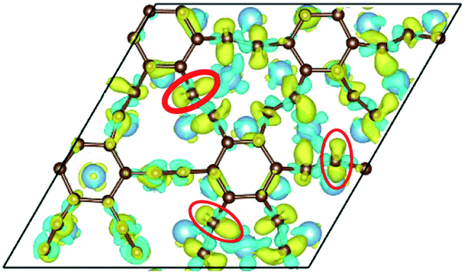 | ||
| Fig. 6 The top view of the differential charge density at the graphyne-Ti (0001) interface. The yellow (red)/blue colors mark an increase/decrease of the charge density, respectively. | ||
It's very essential to calculate the projected density of states to further verify the sd hybridization of the Sc atom, the sd2 hybridization of the Ti atom and the sp3 hybridization of the carbon atom.
As far as the sd hybridization of the Sc atom is concerned, we find that there are significant changes in the densities of states of the C-pz, Sc-s and Sc-d orbitals after adsorption as shown in Fig. 7. In addition, the strong orbital coupling effect is found between the s and d orbitals in the energy range from −2 to 0 eV after adsorption, which proves the s and d orbitals of the Sc atom hybridize with each other in order to form two identical sd orbitals. Moreover, lots of overlapping peaks are found between the C-pz orbital and the Sc-s and Sc-d orbitals below the Fermi energy, that's to say, there exists the strong orbital coupling effect between the C-pz orbital and the Sc-s and Sc-d orbitals, confirming the C-pz orbital forms a covalent bond with one sd orbital of the Sc atom. So does another carbon atom.
 | ||
| Fig. 7 The projected density of states plots of the sd hybridization of the Sc atom corresponding to the local configuration in Fig. 4(a). | ||
Similarly, when it comes to the sd2 hybridization of the Ti atom, numerous overlapping peaks between the Ti-s and Ti-d orbitals as shown in Fig. 8 confirm the strong orbital coupling effect between the s and d orbitals, which shows the s orbital and two d orbitals hybridize with each other in order to three identical sd2-hybridized orbitals and then form three covalent bonds with three carbon atoms.
 | ||
| Fig. 8 The projected density of states plots of the sd2 hybridization of the Ti atom corresponding to the local configuration in Fig. 5(a). | ||
In terms of the sp3 hybridization of the carbon atom, we find the densities of states of the C-s, C-px, C-py, C-pz and Ti-d orbitals change significantly in Fig. 9 after adsorption. Also, there is the strong orbital coupling effect found between the C-s orbital and the C-px, C-py, C-pz orbitals in the energy range from −2 to 0 eV, confirming the C-s orbital and the C-px, C-py, and C-pz orbitals hybridize with each other to form four sp3-hybridized orbitals. Moreover, there are numerous overlapping peaks found between the Ti-d orbital and the C-s, C-px, C-py and C-pz orbitals below the Fermi energy, indicating there exists the strong orbital coupling effect between the Ti-d orbital and the C-s, C-px, C-py and C-pz orbitals. In other words, the carbon atom can form four covalent bonds with the other two carbon atoms and two Ti atoms. The above results verify the rationality of our differential charge density analysis.
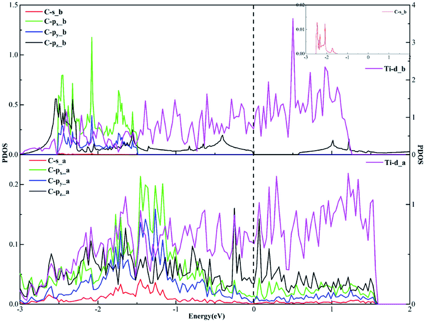 | ||
| Fig. 9 The projected density of states plots of the sp3 hybridization of the C atom corresponding to the local configuration in Fig. 5(b). | ||
Conclusions
We have systematically studied the bonding mechanisms of two-dimensional carbon materials adsorbed on the different transition metal surfaces by means of DFT calculations. The binding energy, the bond length, the differential charge density and the projected density of states were calculated in order to better understand how graphene and graphyne bond with the different transition metals surfaces. The bonding rules of two-dimensional carbon materials adsorbed on the transition metal surfaces are as follows. When a carbon atom is adjacent a metal atom, the pz orbital of the carbon atom that has formed the π-conjunction before adsorption forms a covalent bond with the s orbital or the d orbital of the metal atom directly, such as Ni, Cu and so on. When a metal atom lies below two carbon atoms of graphene or graphyne, the pz orbitals of the two carbon atoms that have formed the π-conjunctions before adsorption form two covalent bonds with two d orbitals of the metal atom directly, such as Ti, Co and so on. However, the Sc atom can't form two covalent bonds directly with two carbon atoms because the Sc atom has only one unpaired d electron. So does the Cu atom. The PDOS results prove that the s orbital and an inner d orbital of the Sc atom hybridize with each other to form two identical sd-hybridized orbitals, and then form two covalent bonds with two pz orbitals of the two carbon atoms. Notably, the two covalent bonds are almost identical by the two sd-hybridized orbital electrons, but the two covalent bonds by the two d-orbital electrons show significant differences. Moreover, three covalent bonds formed between a Ti atom and three carbon atoms are also observed on the graphyne/Ti (0001) interface. This is because the s orbital and two d orbitals of the Ti atom hybridize with each other to form three identical sd2-hybridized orbitals and then form three covalent bonds with the three carbon atoms. In addition to the existing sp and sp2 hybridizations, we also find the carbon atom shows the sp3 hybridization after graphyne adsorbs on the Ti (0001) surface. The PDOS results clearly show the s orbital and three p orbitals (px, py and pz) of the carbon atom hybridize with each other in order to form four sp3-hybridized orbitals. Our results by the present study and previous works systematically elucidate the bonding mechanisms of two-dimensional carbon materials adsorbed on the transition metal surfaces. These research results not only provide help for experimental preparations of two-dimensional carbon materials, but also have vital guiding significance for the applications of two-dimensional carbon materials.Conflicts of interest
There are no conflicts to declare.Acknowledgements
This work was supported by the CAS Frontier Science Research Project (No. QYZDJ-SSW-JSC015) and the National Key R&D Program of China (No. 2016YFB0701302). This work was partially supported by the SYNL Basic Frontier & Technological Innovation Research Project (No. L2019R10). The Special Program for Applied Research on Super Computation of the NSFC-Guangdong Joint Fund (the second phase) are also highly acknowledged. Some of the calculations in this study were done on Tianhe-II high performance computer system in the National Supercomputer Centre in Guangzhou, China.Notes and references
- A. Hirsch, Nat. Mater., 2010, 9, 868–871 CrossRef CAS.
- D. D. L. Chung, J. Mater. Chem., 2002, 37, 1475–1489 CAS.
- H. W. Kroto, J. R. Heath, S. C. O'Brien, R. F. Curl and R. E. Smalley, Nature, 1985, 318, 162–163 CrossRef CAS.
- S. Iijima, Nature, 1991, 354, 56–58 CrossRef CAS.
- K. S. Novoselov, A. K. Geim, S. V. Morozov, D. Jiang, Y. Zhang, S. V. Dubonos, I. V. Grigorieva and A. A. Firsov, Science, 2004, 306, 666 CrossRef CAS.
- A. K. Geim and K. S. Novoselov, Nat. Mater., 2007, 6, 183–191 CrossRef CAS.
- J. Moser, A. Barreiro and A. Bachtold, Appl. Phys. Lett., 2007, 91, 163513 CrossRef.
- D. L. Nika, E. P. Pokatilov, A. S. Askerov and A. A. Balandin, Phys. Rev. B: Condens. Matter Mater. Phys., 2009, 79, 155413 CrossRef.
- A. A. Balandin, Nat. Mater., 2011, 10, 569–581 CrossRef CAS.
- A. S. Mayorov, R. V. Gorbachev, S. V. Morozov, L. Britnell, R. Jalil, L. A. Ponomarenko, P. Blake, K. S. Novoselov, K. Watanabe, T. Taniguchi and A. K. Geim, Nano Lett., 2011, 11, 2396–2399 CrossRef CAS.
- R. Awasthi and R. N. Singh, Carbon, 2013, 51, 282–289 CrossRef CAS.
- W. H. Yuan, Y. J. Gu and L. Li, Appl. Surf. Sci., 2012, 261, 753–758 CrossRef CAS.
- X. Li, J. G. Yu, S. Wageh, A. A. Al-Ghamdi and J. Xie, Small, 2016, 12, 6640–6696 CrossRef CAS.
- W. K. Morrow, S. J. Pearton and F. Ren, Small, 2016, 12, 120–134 CrossRef CAS.
- A. R. Thiruppathi, B. Sidhureddy, E. Boateng, D. V. Soldatov and A. C. Chen, Nanomaterials, 2020, 10, 1295 CrossRef CAS.
- R. G. Ma, Y. Zhou, H. Bi, M. H. Yang, J. C. Wang, Q. Liu and F. Q. Huang, Prog. Mater. Sci., 2020, 113, 100665 CrossRef CAS.
- R. B. Naik, K. V. Reddy, G. M. Reddy and R. A. Kumar, Mater. Lett., 2020, 265, 127437 CrossRef CAS.
- Y. Huang, P. Bazarnik, D. Q. Wan, D. Luo, P. H. R. Pereira, M. Lewandowska, J. Yao, B. E. Hayden and T. G. Langdon, Acta Mater., 2019, 164, 499–511 CrossRef CAS.
- Y. X. Zhao, X. Y. Liu, J. Zhu and S. N. Luo, Phys. Chem. Chem. Phys., 2019, 21, 17393–17399 RSC.
- R. H. Baughman, H. Eckhardt and M. Kertesz, J. Chem. Phys., 1987, 87, 6687–6699 CrossRef CAS.
- G. X. Li, Y. L. Li, H. B. Liu, Y. B. Guo, Y. J. Li and D. B. Zhu, Chem. Commun., 2010, 46, 3256–3258 RSC.
- A. L. Ivanovskii, Prog. Solid State Chem., 2013, 41, 1–19 CrossRef CAS.
- Y. J. Li, L. Xu, H. B. Liu and Y. L. Li, Chem. Soc. Rev., 2014, 43, 2572–2586 RSC.
- Q. Peng, A. K. Dearden, J. Crean, L. Han, S. Liu, X. Wen and S. De, Nanotechnol., Sci. Appl., 2014, 7, 1–29 CAS.
- J. Kang, Z. M. Wei and J. B. Li, ACS Appl. Mater. Interfaces, 2019, 11, 2692–2706 CrossRef CAS.
- D. C. Chen, X. X. Zhang, J. Tang, H. Cui, Y. Li, G. D. Zhang and J. T. Yang, Appl. Surf. Sci., 2019, 465, 93–102 CrossRef CAS.
- Y. Yang, Q. Cao, Y. Gao, S. T. Lei, S. Liu and Q. Peng, RSC Adv., 2020, 10, 1697–1703 RSC.
- Y. Jiao, A. J. Du, M. Hankel, Z. H. Zhu, V. Rudolph and S. C. Smith, Chem. Commun., 2011, 47, 11843–11845 RSC.
- S. W. Cranford and M. J. Buehler, Nanoscale, 2012, 4, 4587–4593 RSC.
- S. Wang, L. X. Yi, J. E. Halpert, X. Y. Lai, Y. Y. Liu, H. B. Cao, R. B. Yu, D. Wang and Y. L. Li, Small, 2012, 8, 265–271 CrossRef CAS.
- H. Ren, H. Shao, L. J. Zhang, D. Guo, Q. Jin, R. B. Yu, L. Wang, Y. L. Li, Y. Wang, H. J. Zhao and D. Wang, Adv. Energy Mater., 2015, 5, 1500296 CrossRef.
- J. Li, X. Gao, B. Liu, Q. L. Feng, X. B. Li, M. Y. Huang, Z. F. Liu, J. Zhang, C. H. Tung and L. Z. Wu, J. Am. Chem. Soc., 2016, 138, 3954–3957 CrossRef CAS.
- P. Wu, P. Du, H. Zhang and C. X. Cai, Phys. Chem. Chem. Phys., 2014, 16, 5640–5648 RSC.
- H. J. Tang, C. M. Hessel, J. Y. Wang, N. L. Yang, R. B. Yu, H. J. Zhao and D. Wang, Chem. Soc. Rev., 2014, 43, 4281–4299 RSC.
- N. L. Yang, Y. Y. Liu, H. Wen, Z. Y. Tang, H. J. Zhao, Y. L. Li and D. Wang, ACS Nano, 2013, 1504–1512 CrossRef CAS.
- L. H. Zhang, S. L. Zhang, P. Wang, C. Liu, S. P. Huang and H. P. Tian, Comput. Theor. Chem., 2014, 1035, 68–75 CrossRef CAS.
- K. Srinivasu and S. K. Ghosh, J. Phys. Chem. C, 2012, 116, 5951–5956 CrossRef CAS.
- Z. Chen, C. Molina-Jirón, S. Klyatskaya, F. Klappenberger and M. Ruben, Ann. Phys., 2017, 529, 1700056 CrossRef.
- C. S. Huang, Y. J. Li, N. Wang, Y. R. Xue, Z. C. Zuo, H. B. Liu and Y. L. Li, Chem. Rev., 2018, 118, 7744–7803 CrossRef CAS.
- Z. Y. Jia, Z. C. Zuo, Y. P. Yi, H. B. Liu, D. Li, Y. J. Li and Y. L. Li, Nano Energy, 2017, 33, 343–349 CrossRef CAS.
- Z. Y. Jia, Y. J. Li, Z. C. Zuo, H. B. Liu, C. S. Huang and Y. L. Li, Acc. Chem. Res., 2017, 50, 2470–2478 CrossRef CAS.
- C. Y. Kuang, G. G. Tang, T. Jiu, H. Yang, H. B. Liu, B. R. Li, W. N. Luo, X. D. Li, W. J. Zhang, F. S. Lu, J. F. Fang and Y. L. Li, Nano Lett., 2015, 15, 2756–2762 CrossRef CAS.
- J. Y. Xiao, J. J. Shi, H. B. Liu, Y. Z. Xu, S. T. Lv, Y. H. Luo, D. M. Li, Q. B. Meng and Y. L. Li, Adv. Energy Mater., 2015, 5, 1401943 CrossRef.
- C. H. Sun and D. J. Searles, J. Phys. Chem. C, 2012, 116, 26222–26226 CrossRef CAS.
- H. Y. Zhang, Y. Y. Xia, H. X. Bu, X. P. Wang, M. Zhang, Y. H. Luo and M. W. Zhao, J. Appl. Phys., 2013, 113, 044309 CrossRef.
- P. Lazić and Ž. Crljen, Phys. Rev. B: Condens. Matter Mater. Phys., 2015, 91, 125423 CrossRef.
- N. N. Han, H. S. Liu, S. Zhou and J. J. Zhao, J. Phys. Chem. C, 2016, 120, 14699–14705 CrossRef CAS.
- Y. Y. Pan, Y. Y. Wang, L. Wang, H. X. Zhong, R. G. Quhe, Z. Y. Ni, M. Ye, W. N. Mei, J. J. Shi, W. L. Guo, J. B. Yang and J. Lu, Nanoscale, 2015, 7, 2116–2127 RSC.
- Y. Q. Tang, H. Y. Yang and P. Yang, Carbon, 2017, 117, 246–251 CrossRef CAS.
- X. Zhang and S. Q. Wang, RSC Adv., 2019, 9, 32712–32720 RSC.
- S. H. Sun, X. Zhang and S. Q. Wang, Mater. Res. Express, 2020, 7, 065603 CrossRef CAS.
- K. Chu, F. Wang, Y. B. Li, X. H. Wang, D. J. Huang and H. Zhang, Carbon, 2018, 133, 127–139 CrossRef CAS.
- K. Chu, F. Wang, X. H. Wang, Y. B. Li, Z. R. Geng, D. J. Huang and H. Zhang, Mater. Des., 2018, 144, 290–303 CrossRef CAS.
- M. Corso, W. Auwärter, M. Muntwiler, A. Tamai, T. Greber and J. Osterwalder, Science, 2004, 303, 217–220 CrossRef CAS.
- J. Wollschläger, D. Erdös, H. Goldbach, R. Höpken and K. M. Schröder, Thin Solid Films, 2001, 400, 1–8 CrossRef.
- G. Kresse and J. Furthmüller, Comput. Mater. Sci., 1996, 6, 15–50 CrossRef CAS.
- J. P. Perdew and A. Zunger, Phys. Rev. B: Condens. Matter Mater. Phys., 1981, 23, 5048–5079 CrossRef CAS.
- M. Vanin, J. J. Mortensen, A. K. Kelkkanen, J. M. Garcia-Lastra, K. S. Thygesen and K. W. Jacobsen, Phys. Rev. B: Condens. Matter Mater. Phys., 2010, 81, 081408(R) CrossRef.
- G. Kresse and D. Joubert, Phys. Rev. B: Condens. Matter Mater. Phys., 1999, 59, 1758–1775 CrossRef CAS.
- P. E. Blöchl, O. Jepsen and O. K. Andersen, Phys. Rev. B: Condens. Matter Mater. Phys., 1994, 49, 16223–16233 CrossRef.
- J. Neugebauer and M. Scheffler, Phys. Rev. B: Condens. Matter Mater. Phys., 1992, 46, 16067–16080 CrossRef CAS.
- Z. Xu, Q. B. Yan, Q. R. Zheng and G. Su, Phys. Rev. B: Condens. Matter Mater. Phys., 2009, 80, 081306 CrossRef.
- T. Akiyama, K. Nakamura and T. Ito, Phys. Rev. B: Condens. Matter Mater. Phys., 2006, 73, 235308 CrossRef.
- H. B. Shu, X. S. Chen, Z. L. Ding, R. B. Dong and W. Lu, J. Phys. Chem. C, 2011, 115, 14449–14454 CrossRef CAS.
| This journal is © The Royal Society of Chemistry 2020 |