 Open Access Article
Application and interpretation of deep learning methods for the geographical origin identification of Radix Glycyrrhizae using hyperspectral imaging
Tianying Yan ab,
Long Duanab,
Xiaopan Chena,
Pan Gao
 *ab and
Wei Xu*cd
aCollege of Information Science and Technology, Shihezi University, Shihezi 832003, China. E-mail: gp_inf@shzu.edu.cn
bKey Laboratory of Oasis Ecology Agriculture, Shihezi University, Shihezi 832003, China
cCollege of Agriculture, Shihezi University, Shihezi 832003, China. E-mail: xuwei0412@shzu.edu.cn
dXinjiang Production and Construction Corps Key Laboratory of Special Fruits and Vegetables Cultivation Physiology and Germplasm Resources Utilization, Shihezi 832003, China
First published on 18th November 2020
Abstract
Radix Glycyrrhizae is used as a functional food and traditional medicine. The geographical origin of Radix Glycyrrhizae is a determinant factor influencing the chemical and physical properties as well as its medicinal and health effects. The visible/near-infrared (Vis/NIR) (376–1044 nm) and near-infrared (NIR) hyperspectral imaging (915–1699 nm) were used to identify the geographical origin of Radix Glycyrrhizae. Convolutional neural network (CNN) and recurrent neural network (RNN) models in deep learning methods were built using extracted spectra, with logistic regression (LR) and support vector machine (SVM) models as comparisons. For both spectral ranges, the deep learning methods, LR and SVM all exhibited good results. The classification accuracy was over 90% for the calibration, validation, and prediction sets by the LR, CNN, and RNN models. Slight differences in classification performances existed between the two spectral ranges. Further, interpretation of the CNN model was conducted to identify the important wavelengths, and the wavelengths with high contribution rates that affected the discriminant analysis were consistent with the spectral differences. Thus, the overall results illustrate that hyperspectral imaging with deep learning methods can be used to identify the geographical origin of Radix Glycyrrhizae, which provides a new basis for related research.
1. Introduction
Glycyrrhiza is a perennial herb with a thick rhizome, and its medicinal parts are the root and rhizome.1,2 As a therapeutic part of Glycyrrhiza, Radix Glycyrrhizae is a type of traditional Chinese functional food and the most common clinical medicine. Radix Glycyrrhizae is widely welcomed in China, Japan, and Korea because it can clear the heat and detoxify, moisten the lungs, relieve cough, and replenish the spleen and shortness of breath.3–5 Radix Glycyrrhizae contains complex chemical compositions, including glycyrrhizin, glycyrrhetinic acid, liquiritigenin, isoliquiritigenin, and neoliquiritigenin.6,7Glycyrrhiza grows mostly in the arid and semi-arid desert steppe, desert edge, and loess hilly area, such as Gansu Province, China; Inner Mongolia Autonomous Region, China; Ningxia Hui Autonomous Region, China; and Xinjiang Uygur Autonomous Region, China. The content of the chemical components of Radix Glycyrrhizae affects its quality;8 different natural conditions in different geographical origins such as soil, water quality, climate, sunshine, and rainfall lead to variations in its quality. For example, the glycyrrhizic acid content of Radix Glycyrrhizae in Shihezi City (Xinjiang Uygur Autonomous Region, China) is 0.2%, while that in Tongliao City (Inner Mongolia Autonomous Region, China) is 5.82%. The difference in glycyrrhizic acid in Radix Glycyrrhizae between these two geographical origins is nearly 30 times.4,5 At present, the global demand for Radix Glycyrrhizae is gradually increasing. Although the planting area of Radix Glycyrrhizae is extensive, its geographical origins on the market are complex, and the quality of medicinal materials is varied. Therefore, the identification of Radix Glycyrrhizae from different geographical origins is essential for its quality evaluation.
Traditional methods for identifying the geographical origins of Radix Glycyrrhizae include the experience-based and chemical analysis-based methods. Experience-based methods are based on the experience of planters and consumers. For example, experienced experts can distinguish the origin of Radix Glycyrrhizae by its shape, color, and taste. These experience-based methods require greater experience by experts, and their accuracy cannot be controlled. The chemical analysis methods, such as high-performance liquid chromatography (HPLC),9,10 thin layer chromatography (TLC),11 and other methods are practical tools to identify the geographical origin of Radix Glycyrrhizae. Although these methods can successfully identify the geographical origins of Glycyrrhiza Glycyrrhizae, they are limited to destructive sampling, complex processing, and high technical requirements, which lead to a low identification efficiency. These methods are unable to achieve large-scale identification and detection.
Computer vision has attracted wide attention in non-destructive testing. As a non-chemical and non-destructive technique, computer vision has advantages in identifying samples with significant differences in external characteristics. However, although computer vision offers suitable recognition of changes in morphology and texture, it is unable to give information regarding internal composition. In contrast, near-infrared (NIR) spectroscopy has unique advantages in obtaining spectral information related to internal components. It has been widely used in the detection of different varieties and origins of agricultural products.12,13 However, spectroscopy can only obtain spectral information from a certain point in samples. Accordingly, hyperspectral imaging (HSI) combines the advantages of computer vision and spectroscopy techniques. It has become an effective analytical technique, and the spatial and spectral information of the detected object can be obtained simultaneously by HSI. Therefore, HSI can get both external characteristic information and internal molecular information of samples, providing the possibility for the comprehensive analysis of samples. In recent years, the quality assessment and variety classification of HSI in the fields of agriculture14–16 and food17–22 have attracted increasing attention. It is possible to rapidly and accurately identify the geographical origins of Radix Glycyrrhizae through HSI.
Effective analysis of massive data acquired by hyperspectral imaging is a great challenge, thus hindering its application. Therefore, it is essential to select appropriate and efficient data analysis and processing methods to make full use of HSI. At present, machine learning is considered to be the best choice for complex data processing and analysis. As a new research direction of machine learning, deep learning has a better effect on image and spectral processing.23,24 Deep learning has strong self-learning, feature extraction, and large-scale data processing capabilities. It realizes fast and efficient data analysis by constructing a network composed of a large number of neurons. Due to its unique self-learning ability and excellent performance, deep learning has been widely welcomed by researchers and applied for the processing of spectroscopy.25–28 However, deep learning is also controversial. It has been used as a black box. Its performance is outstanding, and its interpretability is very important. One possible way is to sequentially calculate and visualize the feature maps of the network layer, but the deep feature maps are difficult to understand.29 Another way is to use the gradient backpropagation in the deep learning process, and finally get the gradient value of the same size as the input data. According to the gradient value, the regions of interest in the deep learning process can be explained well.30,31 Therefore, when deep learning methods are used, interpretable visualization methods should also be used.
To the best of our knowledge, no studies have been reported on the application of HSI in the identification of the geographical origins of Radix Glycyrrhizae. Therefore, this study aimed to propose a method to quickly and accurately identify the geographical origins of Radix Glycyrrhizae by collecting hyperspectral images and using deep learning for its classification and discovering important wavelengths. The specific objectives achieved herein are as follows:
(1) Visible/near-infrared (Vis/NIR) and NIR hyperspectral imaging systems were explored for the feasibility of identifying the geographical origins of Radix Glycyrrhizae.
(2) The effectiveness of statistically-based machine learning methods and deep learning methods in distinguishing the geographical origins of Radix Glycyrrhizae was compared.
(3) To discover the important wavelengths of Vis/NIR spectra and NIR spectra contributing more to the classification, the feasibility of applying interpretable visualization methods to convolutional neural network (CNN) models was discussed.
2. Materials and methods
2.1 Sample preparation
Radix Glycyrrhizae samples were obtained from four different geographical origins, including Gansu Province (Gansu), China (92°13′–108°46′ E, 32°31′–42°57′ N); Inner Mongolia Autonomous Region (Inner Mongolia), China (97°12′–126°04′ E, 37°24′–53°23′ N); Ningxia Hui Autonomous Region (Ningxia), China (104°17′–109°39′ E, 35°14′–39°14′ N); and Xinjiang Uygur Autonomous Region (Xinjiang), China (73°40′–96°18′ E, 34°25′–48°10′ N). The samples from each geographical origin were air-dried for sale and trade and collected in May 2020 for the experiment. The samples were cleaned, prepared, and dried with no significant differences in their shape and appearance.A total of 2600 samples were collected, and the number of Radix Glycyrrhizae samples from each geographical origin was the same. To establish the classification models, the samples were randomly divided into the calibration, validation, and prediction sets. The ratio of the number of samples in the calibration, validation, and prediction sets was 3![[thin space (1/6-em)]](https://www.rsc.org/images/entities/char_2009.gif) :
:![[thin space (1/6-em)]](https://www.rsc.org/images/entities/char_2009.gif) 1
1![[thin space (1/6-em)]](https://www.rsc.org/images/entities/char_2009.gif) :
:![[thin space (1/6-em)]](https://www.rsc.org/images/entities/char_2009.gif) 1. In each set, the number of samples of Radix Glycyrrhizae from the four geographical origins was almost equal, with slight differences due to the codes in Python.
1. In each set, the number of samples of Radix Glycyrrhizae from the four geographical origins was almost equal, with slight differences due to the codes in Python.
2.2 Hyperspectral image acquisition and correction
In this study, two hyperspectral imaging systems (Vis/NIR and NIR hyperspectral imaging systems) were used to photograph cross-sections of the Radix Glycyrrhizae samples from four geographical origins. Both the Vis/NIR and NIR hyperspectral imaging systems were composed of four modules, including an imaging module, illumination module, lift module, and software module. The imaging module consisted of the Surface Optics Corporation (SOC) 710 series cameras (Surface Optics Corporation, San Diego, California, USA). The cameras had internal scanning mechanisms so that they could scan in any direction or directly vertically downward without the need for an additional scanning table. The Vis/NIR hyperspectral imaging system (SOC 710VP) had a spectral wavelength range of 376–1044 nm, spectral resolution of 5 nm, and number of wavebands of 128. The NIR hyperspectral imaging system (SOC 710SWIR) had a spectral wavelength range of 915–1699 nm, spectral resolution of 2.7 nm, and number of wavebands of 288. Halogen lamps were used as the lighting module, the power of a single halogen lamp was 50 W, and a total of 4 halogen lamps was employed. The lifting platform module placed the shooting object, and the imaging module could fully capture the shooting object by lifting. The software module was used to control HSI acquisition.The size of the image collected by the Vis/NIR hyperspectral imaging system was 128 wavebands × 520 pixels × 696 pixels, and the size of the image collected by the NIR hyperspectral imaging system was 288 wavebands × 512 pixels × 640 pixels. The data storage method of HSI was waveband number × pixel width × pixel length. During the shooting process, the sample was fully captured by the imaging module by controlling the lifting platform. The distance between the imaging module of the hyperspectral imaging systems and the samples was 89 cm. The exposure time of SOC 710VP was 25 ms, and the exposure time of SOC 710SWIR was 34 ms. The internal scanning speed of the SOC series cameras automatically matched their exposure time. In this study, the gray (combined with 50% black and 50% white) board provided by SOC was photographed and the gray reference image was obtained. 50 samples of Radix Glycyrrhizae from the same geographical origin were placed on a blackboard and then photographed. After HSI acquisition, the original hyperspectral images were corrected to reflectance images according to eqn (1).
 | (1) |
2.3 Spectral data extraction
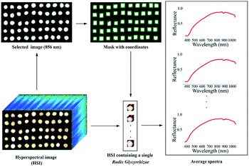
Considering the obvious electrical signal noise during the photographing process, the image was preprocessed by the Savitzky–Golay (SG) smoothing filter (the kernel size was 5 × 5 × 5, the polynomial order was 3, and the filter calculated the filtered value at the central node of the kernel) to reduce random noise. The image of one wavelength in HSI was used as a mask, and the coordinates of a single Radix Glycyrrhizae were identified based on the mask. The sub-HSIs containing only a single Radix Glycyrrhizae were extracted one by one according to the coordinates. In the sub-HSIs containing only a single Radix Glycyrrhizae, the Radix Glycyrrhizae region was regarded as the region of interest (ROI), and the average spectrum of the ROI was calculated. The wavelength image at 856 nm of the reflectance image acquired by the Vis/NIR imaging system and the image at 1109 nm wavelength of the reflectance image acquired by the NIR imaging system were used as the mask. The coordinates of the mask containing a single Radix Glycyrrhizae were calculated. According to the coordinates, the sub-HSIs containing a single Radix Glycyrrhizae were extracted from the hyperspectral image. The Radix Glycyrrhizae in the sub-HSIs was regarded as the ROI, and its average spectrum was extracted and calculated. The spectra of the area outside ROI were not extracted and calculated. The spectra extraction process is shown in Fig. 1.2.4 Data analysis methods
| Sc(SPEC) ≈ wTcSPEC + b | (2) |
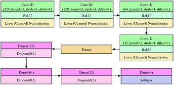
In this study, layer (channel) normalization was used for the 1D CNN model. Normalization could speed up model convergence. For the spectra, the size of the feature map output during the training process was N × C × W, where N represents the number of spectra participating in the training, C represents the number of channels, and W represents the number of wavebands of the spectra. Under the initial conditions, the spectra could be regarded as a feature map, and the number of channels was 1.
The CNN architecture is shown in Fig. 2. It consists of four main parts. The first part includes four 1D convolutional layers (Conv1D, green box), and each layer is followed by a ReLU (rectified linear unit) activation layer (light blue box) and a normalization (channel) layer (light brown box). The second part is the flatten layer. The third part includes a fully connected network consisting of three dense layers (dark red boxes) and three dropout layers (light red boxes). The last part consists of a dense layer and a softmax layer (dark blue box). The numbers of kernels in the convolutional layers were 256, 128, 64, and 32 respectively, the kernel size was 3, the stride was 1, and the dilate was 1 without padding. In the dense layer, the number of neurons was defined as 128, 64, 32, and 4 in sequence. The dropout layer was set to a probability of 0.2.
The training process of CNN was implemented using the stochastic gradient descent (SGD) algorithm to minimize the softmax cross-entropy loss, and the learning rate was set to 0.01. The Xavier method was used to initialize the parameters. The batch size was set to 100, and the epoch size was defined as 300.
 | (3) |
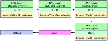
In this study, the instance (width) normalization was used for the RNN model. For the spectral data, the size of the feature map output during the training process was similar to that of CNN. The RNN model was employed to explore the correlation between wavelengths and see if it could improve the classification results.
The RNN architecture is shown in Fig. 3. It consists of three main parts. The first part consists of three RNN_layers (green box), and each layer is followed by an ReLU activation layer (light blue box) and an instance (width) normalization layer (light brown box). The second part is a fully connected network consisting of a dense layer (dark red box). The last part consists of the softmax layer (dark blue box). The number of the RNN_layer was 1, and the numbers of features in the hidden state were 256, 128, 64, and 32, respectively. In the dense layer, the number of neurons was defined as 4. The training process of RNN adopted the same strategy as CNN.
Given a spectrum SPEC0 of category c in the prediction set, after being classified by the 1D CNN model, the score value Sc would be obtained. If the predicted category was consistent with the true category, the effective weights of all wavebands could be calculated. The calculation process was carried out according to eqn (4).
 | (4) |
In this study, each wavelength in the spectra sorted from small to large was sequentially numbered with a natural number starting from 1, and the number was the number of wavebands.
The index B* of the wavebands with the maximum weight value was counted in all the correctly classified samples, as shown in eqn (5).
 | (5) |
Among them, eqn (5) counts the index of the maximum value in all j wavebands of each sample, where SPECi is the i-th sample correctly classified in the prediction set of SPEC, and N(SPECi,B) is the waveband weight of the i-th sample correctly classified in the prediction set.
In this study, the spectral ranges were discrete, depending on the spectral resolution of the cameras. In the effective spectral ranges of the cameras (the spectra at the head and tail of the noise were removed), the waveband index value at the beginning of the effective spectra was numbered 1. The effective spectral wavelength increased in sequence according to the spectral resolution of the cameras, and the corresponding waveband index number increased in sequence by 1. The index value of the waveband with the maximum weight value of each correctly classified sample was recorded as B*, and the frequency of each index value in B* was counted. The frequency of the waveband index values reflected the importance of the waveband, and the important wavelengths corresponding to the index values of the waveband were discovered.
2.5 Software and model evaluation
In this study, the Python scripting language (version 3.7.6, 64 bit) was used for the numerical calculations. LR and SVM were implemented on the machine learning library software scikit-learn (version 0.23.1), which was used to divide the data set, and the random state was set to 1. The 1D CNN and RNN models were built on the deep learning MXNet (version 1.5.0) framework (Amazon, Seattle, Washington State, USA). All machine learning algorithms used the calibration set for learning and the validation set accuracy for optimizing the algorithm parameters. The corresponding optimal models were saved and evaluated to classify the prediction set. The classification accuracy was used to evaluate the model performances, which was calculated as the ratio of the number of correctly classified samples to the total number of samples.3. Results and discussion
3.1 Spectral profiles
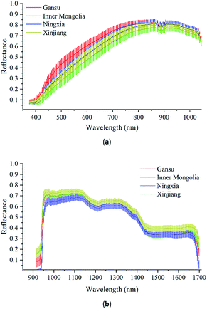
Fig. 4(a) shows the Vis/NIR average spectra (376–1044 nm) and standard deviation for each wavelength of Radix Glycyrrhizae from Gansu, Inner Mongolia, Ningxia, and Xinjiang. Fig. 4(b) shows the corresponding NIR average spectra (915–1699 nm) and the standard deviation. In the Vis/NIR and NIR average spectra of Radix Glycyrrhizae of each category, the spectral curves were similar, and there were differences in the entire wavelengths. The standard deviations of the spectral values at each wavelength did not overlap significantly. The classification model could be further employed to identify samples from different geographical origins according to the differences existing in their spectra.The hyperspectral images collected by the two hyperspectral imaging systems had obvious noise at the beginning of the wavelengths, and there was a small amount of noise at the end of the spectra. In this study, the Vis/NIR spectra in the spectral range of 421–1044 nm and the NIR spectra in the spectral range of 951–1680 nm were used to build the models to identify the geographical origins of Radix Glycyrrhizae.
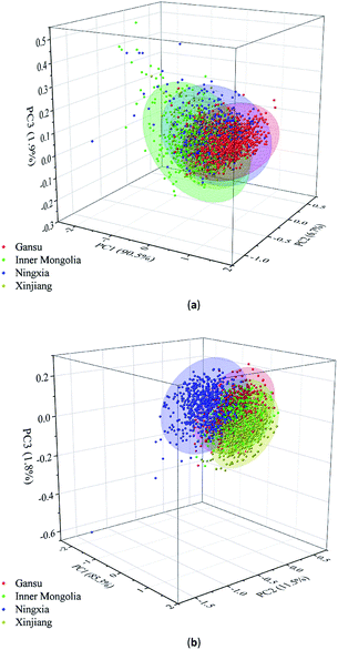
According to Fig. 4(a) and (b), it can be seen that the spectra of the Radix Glycyrrhizae samples from different geographical origins are gathered together and separated in large spectral ranges. PCA was used to explore the differences in the Radix Glycyrrhizae from the different geographical origins. In the 3D PCA score plot of the Vis/NIR average spectra, the first three PCs explained 90.5%, 6.7% and 1.9% of the total variance of the data set, respectively. In the 3D PCA score plot of the NIR average spectra, the first three PCs explained 85.3%, 11.5% and 1.8% of the total variance of the data set, respectively. The results showed that most of the spectral information related to the samples was involved. The 3D PCA score plots (X-axis: PC1, Y-axis: PC2, and Z-axis: PC3) are shown in Fig. 5(a) and (b). Radix Glycyrrhizae of each geographical origin is displayed in a different color to achieve better visualization. In the 3D PCA score plots of the Vis/NIR average spectra and NIR average spectra, it can be observed that the samples of each geographical origin are grouped, but there is overlap between the samples of different geographical origins, and several samples are far away from the cluster center. In general, PCA can provide an overview of the sample distribution, but it cannot provide clear enough discrimination. Therefore, other classification methods should be considered.
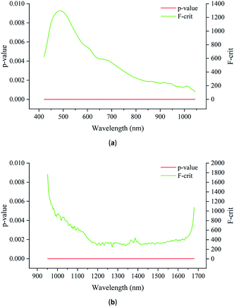
To further investigate the differences in the spectra, analysis of variance (ANOVA) was used to explore the differences among the Radix Glycyrrhizae from different geographical origins. Fig. 6(a) shows the F-critical value and p-value of each wavelength of Vis/NIR. Fig. 6(b) shows the F-critical value and p-value of each wavelength of NIR.
For both the Vis/NIR and NIR spectra, the p-value of all the wavelengths was less than 0.05. This shows that the spectral values of all wavelengths of Radix Glycyrrhizae from different geographical origins were significantly different. The minimum F-critical value and the maximum F-critical value did not exceed one order of magnitude, and each wavelength had the potential to be used to distinguish the geographical origins of Radix Glycyrrhizae. The F-critical value from the Vis/NIR spectral range of 440–540 nm, and the F-critical value from the NIR spectral range of 950–1040 nm were significantly higher than that in the other spectral regions.
3.2 Classification models using full spectra
The deep learning methods CNN and RNN were used to build classification models, and the LR and SVM models were used for comparison. To build the LR, SVM, CNN, and RNN models, the spectra without noise wavelengths were used. To build the classification models, the category values of the samples from Gansu, Inner Mongolia, Ningxia, and Xinjiang were marked as 0, 1, 2, and 3, respectively.For the two different spectral ranges, the classification results of the four different models are shown in Table 1. All the discriminant models were optimized by the Bayesian optimization algorithm. The number of iterations of the optimization algorithm was 200.
| Module | Method | Category value | Calibration | Validation | Prediction | ||||||||||||
|---|---|---|---|---|---|---|---|---|---|---|---|---|---|---|---|---|---|
| 0 | 1 | 2 | 3 | Accuracy (%) | 0 | 1 | 2 | 3 | Accuracy (%) | 0 | 1 | 2 | 3 | Accuracy (%) | |||
| a VP means the spectra were extracted and calculated from the hyperspectral image collected by the SOC 710VP imaging module. SWIR means the spectra were extracted and calculated from the hyperspectral image collected by the SOC 710SWIR imaging module.b 0, 1, 2, and 3 are the assigned category values of the samples from Gansu, Inner Mongolia, Ningxia, and Xinjiang, respectively. | |||||||||||||||||
| VPa | LR | 0b | 387 | 1 | 2 | 1 | 127 | 1 | 129 | 1 | |||||||
| 1 | 1 | 314 | 8 | 60 | 115 | 3 | 19 | 1 | 113 | 1 | 15 | ||||||
| 2 | 1 | 4 | 381 | 2 | 3 | 129 | 129 | 1 | |||||||||
| 3 | 47 | 3 | 348 | 1 | 10 | 3 | 108 | 7 | 4 | 119 | |||||||
| Total | 91.67 | 92.12 | 94.23 | ||||||||||||||
| SVM | 0 | 391 | 124 | 4 | 1 | 126 | 1 | 2 | 1 | ||||||||
| 1 | 383 | 2 | 109 | 3 | 23 | 1 | 106 | 2 | 21 | ||||||||
| 2 | 388 | 1 | 11 | 112 | 8 | 7 | 3 | 119 | 1 | ||||||||
| 3 | 398 | 0 | 19 | 5 | 98 | 4 | 20 | 3 | 103 | ||||||||
| Total | 100.00 | 85.19 | 87.31 | ||||||||||||||
| CNN | 0 | 391 | 128 | 1 | 130 | ||||||||||||
| 1 | 383 | 119 | 3 | 15 | 112 | 18 | |||||||||||
| 2 | 388 | 132 | 1 | 128 | 1 | ||||||||||||
| 3 | 398 | 7 | 1 | 114 | 7 | 123 | |||||||||||
| Total | 100.00 | 94.81 | 94.81 | ||||||||||||||
| RNN | 0 | 391 | 124 | 2 | 2 | 1 | 128 | 1 | 1 | ||||||||
| 1 | 383 | 118 | 2 | 17 | 119 | 1 | 10 | ||||||||||
| 2 | 388 | 3 | 129 | 1 | 129 | ||||||||||||
| 3 | 25 | 373 | 16 | 106 | 28 | 3 | 99 | ||||||||||
| Total | 98.40 | 91.73 | 91.35 | ||||||||||||||
| SWIR | LR | 0 | 386 | 5 | 123 | 1 | 5 | 128 | 1 | 1 | |||||||
| 1 | 383 | 137 | 127 | 3 | |||||||||||||
| 2 | 1 | 387 | 132 | 130 | |||||||||||||
| 3 | 5 | 1 | 392 | 3 | 119 | 1 | 1 | 128 | |||||||||
| Total | 99.23 | 98.27 | 98.65 | ||||||||||||||
| SVM | 0 | 390 | 1 | 117 | 1 | 3 | 8 | 127 | 1 | 1 | 1 | ||||||
| 1 | 382 | 1 | 2 | 130 | 5 | 1 | 121 | 8 | |||||||||
| 2 | 6 | 2 | 380 | 1 | 131 | 1 | 129 | ||||||||||
| 3 | 12 | 1 | 385 | 14 | 2 | 106 | 7 | 5 | 118 | ||||||||
| Total | 98.53 | 93.08 | 95.19 | ||||||||||||||
| CNN | 0 | 391 | 128 | 1 | 129 | 1 | |||||||||||
| 1 | 383 | 137 | 3 | 123 | 4 | ||||||||||||
| 2 | 388 | 1 | 131 | 130 | |||||||||||||
| 3 | 398 | 1 | 121 | 7 | 123 | ||||||||||||
| Total | 100.00 | 99.42 | 97.12 | ||||||||||||||
| RNN | 0 | 391 | 124 | 2 | 3 | 130 | |||||||||||
| 1 | 381 | 2 | 1 | 135 | 1 | 3 | 124 | 3 | |||||||||
| 2 | 388 | 132 | 130 | ||||||||||||||
| 3 | 398 | 5 | 117 | 130 | |||||||||||||
| Total | 99.87 | 97.69 | 98.85 | ||||||||||||||
For the Vis/NIR spectra, all the models had good performances, with the classification accuracy of the calibration, validation and prediction sets all exceeding 85%. The LR, CNN, and RNN models showed close results, and the SVM model showed relatively lower results. For the LR model, the L2 paradigm was used as the loss function, and the model parameters (C, solver) were set to (1.957, ‘liblinear’), and its classification accuracy in the calibration, validation, and prediction sets exceeded 90%. For the SVM model, the final model parameters (kernel, gamma, C) were optimized to (‘poly’, 17.313, 1.864). The classification accuracy of the calibration set was 100.00%, while the classification accuracy of the validation set and prediction set was found to be lower. For the CNN model, the classification accuracy of the calibration, validation, and prediction sets was all over 94%. For the RNN model, the classification accuracy of the calibration, validation, and prediction sets was all over 91%.
For the NIR spectra, the classification accuracy of the calibration, validation, and prediction sets in all models exceeded 87%. The LR, CNN and RNN models showed close results, and the SVM model showed relatively lower results. For the LR model, the model parameters (C, solver) were set to (1.856, ‘liblinear’), and its classification accuracy in the calibration, validation, and prediction sets exceeded 98%. For the SVM model, the model parameters (kernel, gamma, C) were optimized to (‘poly’, 0.052, 1.700), and the classification accuracy in each data set exceeded 93%. For the CNN and RNN models, the classification accuracy of the calibration, validation, and prediction sets was all over 97%. Thus, the combination of Vis/NIR and NIR hyperspectral imaging and deep learning methods can be used to identify the geographical origins of Radix Glycyrrhizae.
As shown in Table 1, the classification results of each model showed close results in the two spectral ranges, and the results were all acceptable. Thus, the results illustrate the feasibility of using the hyperspectral imaging in the two spectral ranges for the geographical origin identification of Radix Glycyrrhizae. The classification performances of the deep learning methods (CNN and RNN) were equivalent to or better than the LR and SVMs, indicating the effectiveness of deep learning methods for the geographical origin identification of Radix Glycyrrhizae. The overall results indicated that the combination of Vis/NIR and NIR hyperspectral imaging and deep learning methods can be used to identify the geographical origins of Radix Glycyrrhizae.
3.3 Visualization for discovering important wavelengths
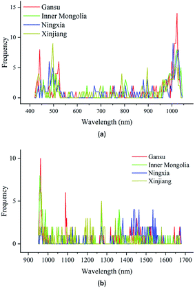
For the classification of the geographical origins of Radix Glycyrrhizae, it is important to know which wavelengths contribute more to the classification results. In this study, after the LR model learned the calibration set, it had a fixed weight w and deviation b, and the model parameters reflected the overall evaluation of the modeling set. It was difficult to find the important wavelengths that contribute more to distinguish different types of spectra. Even if the gradient was solved backward for the classification results, the gradients of all the spectra were constant. SVM looked for a classification hyperplane to separate different types of data, and the basis of the separation was the support vectors. The support vectors were the typical spectra of each category in the calibration set. Regardless of the weight w and gradient, it was difficult to find the important wavelengths of the spectra. The gradient clipping algorithm was used in RNN. It was difficult to find the important wavelengths of the spectra based on the weight and gradient. The weight sharing of CNN did not affect the gradient calculation. Also, the saliency map was a reliable way to interpret the model. It could be used to find the important wavelengths of the CNN model.For the Vis/NIR spectra and NIR spectra, the gradient was calculated according to eqn (4), and the important wavelengths were found according to eqn (5). The frequency of the wavelength with the largest gradient of all samples in the prediction set correctly predicted by the CNN model was calculated. The frequency reflected the influence of wavelength on the identification results in the modeling process. High-frequency wavelengths were more likely to affect the identification results. Thus, these wavelengths were considered important. The important wavelengths of the Vis/NIR and NIR spectra of each geographical origin could be observed intuitively, as shown in Fig. 7. The ordinates in Fig. 7(a) and (b) represent the frequency of the wavelength with the largest gradient of all the correctly classified samples in the prediction set by the CNN model.
As seen in Fig. 7(a), the important wavelengths for distinguishing Radix Glycyrrhizae from different geographical origins are mainly concentrated in the range of 440–540 nm and 950–1040 nm. The wavelengths between 540 and 950 nm had little effect on the classification results. It can be seen from Fig. 7(b) that the wavelengths that have the greatest impact on the classification results are mainly concentrated in the range of 951–1000 nm, 1430–1560 nm, 1320–1380 nm, and around 1100 and 1275 nm. The remaining wavelengths had roughly the same and lower influence on the classification result. These results were matched with the results of ANOVA (Fig. 6). In the range of the Vis spectra, 440–540 nm, involving the blue, cyan, and green Vis spectral range, had a greater impact on the classification results. This may be related to the subtle color differences of Radix Glycyrrhizae from different geographical origins. In the range of the NIR spectra, the wavelengths between 950 nm and 1040 nm represent the second overtone of the O–H stretching vibrations.44 The wavelengths of 1100 nm and 1275 nm can be assigned to the second overtone associated with the C–H stretching vibrations.45,46 The wavelengths in the range of 1320–1380 nm can be attributed to the third overtone and the combination of C–H stretching vibrations.47 The wavelengths in the range of 1430–1560 nm are due to the first overtone of the O–H stretching vibrations. These may be related to the compounds contained in Radix Glycyrrhizae, such as glycyrrhizin, glycyrrhetinic acid and liquiritigenin.
To evaluate the effectiveness of the identified important wavelengths, they were used to build the CNN model. For the spectra in the selected Vis/NIR wavelengths, the classification accuracy of the calibration, validation, and prediction sets was 94.04%, 90.38%, and 90.77%, respectively. For the spectra in the selected NIR wavelengths, the classification accuracy of the calibration, validation, and prediction sets was 99.94%, 96.15%, and 96.15%, respectively. Among them, the number of wavebands of the Vis/NIR spectra was reduced to about 32% of the total wavebands, and the classification accuracy of the validation and prediction sets was roughly reduced by 4.43% and 4.04%, respectively. The number of wavebands of the NIR spectra was reduced to about 35% of the total wavebands, and the classification accuracy of validation and prediction sets was reduced by about 3.27% and 0.97%, respectively. This shows that the visualization method applied to CNN can discover important wavelengths and provide new directions for feature selection.
4. Conclusions
In this study, a Vis/NIR hyperspectral imaging system (376–1044 nm) and NIR hyperspectral imaging system (915–1699 nm) were successfully used to identify the geographical origins of Radix Glycyrrhizae from Gansu, Inner Mongolia, Ningxia, and Xinjiang. The LR, SVM, CNN, and RNN models were established using the Vis/NIR and NIR spectra. For the models using the Vis/NIR spectra, the classification accuracy of the worst-performing classifier in different datasets exceeded 85%. The CNN model performed best, with the classification accuracy of over 94%, followed by the LR and RNN models. For the models using NIR spectra, the LR, CNN, and RNN models obtained a classification accuracy of over 93% in the calibration, validation, and prediction sets. The LR, CNN, and RNN models had similar abilities to identify the geographical origins in the two different spectral ranges. The classification performances of the SVM model were the worst. The results showed that Vis/NIR and NIR hyperspectral imaging combined with deep learning could be used to distinguish different geographical origins of Radix Glycyrrhizae. Besides, the interpretable saliency map was used to visualize the CNN model, and the important wavelengths contributing more to the classification found by the visualization were matched with that identified in ANOVA of the original spectra. The important wavelengths were selected and remodeled by CNN. Based on reducing the number of spectral wavebands by at least 35%, the classification accuracy of the validation and prediction sets was only reduced by up to 4.43%, and the classification accuracy of CNN exceeded 90%. Thus, the overall results provide a new perspective for the geographical origin identification of Radix Glycyrrhizae, as well as a method to identify important wavelengths for its identification.Conflicts of interest
There are no conflicts to declare.Acknowledgements
This research was funded by the National Natural Science Foundation of China, grant number 61965014, and the Scientific and Technological Research Projects in Key Areas of Xinjiang Production and Construction Corps (XPCC), grant number 2020AB005.References
- Y. Sato, J. X. He, H. Nagai, T. Tani and T. Akao, Biol. Pharm. Bull., 2007, 30, 145–149, DOI:10.1248/bpb.30.145.
- H. K. Lee, E. J. Yang, J. Y. Kim, K. S. Song and Y. H. Seong, Arch. Pharmacal Res., 2012, 35, 897–904, DOI:10.1007/s12272-012-0515-y.
- M. Chen, D. Geng, X. Yang, X. Liu, S. Liu, P. Ding, Y. Pang, M. Du, X. Hu and R. Wang, Oxid. Med. Cell. Longevity, 2020, 2020, 6894751, DOI:10.1155/2020/6894751.
- Y. Guo, L. Xu, S. Wu, P. Meng, Q. Qiu, L. Li and X. Song, J. Guangzhou Univ. Tradit. Chin. Med., 2020, 37, 190–194 Search PubMed.
- W. Xie, F. Zeng and C. Lv, Chinese Medicine Modern Distance Education of China, 2019, 17, 92–93 Search PubMed.
- J. Kamei, R. Nakamura, H. Ichiki and M. Kubo, Eur. J. Pharmacol., 2003, 469, 159–163, DOI:10.1016/s0014-2999(03)01728-x.
- J. Kamei, A. Saitoh, T. Asano, R. Nakamura, H. Ichiki, A. Iiduka and M. Kubo, Eur. J. Pharmacol., 2005, 507, 163–168, DOI:10.1016/j.ejphar.2004.11.042.
- Y. A. Woo, H. J. Kim, J. Cho and H. Chung, J. Pharm. Biomed. Anal., 1999, 21, 407–413, DOI:10.1016/s0731-7085(99)00145-4.
- P. K. Sahu, N. R. Ramisetti, T. Cecchi, S. Swain, C. S. Patro and J. Panda, J. Pharm. Biomed. Anal., 2018, 147, 590–611, DOI:10.1016/j.jpba.2017.05.006.
- W. Wei, J. Li and L. Huang, Czech J. Food Sci., 2017, 35, 40–47, DOI:10.17221/126/2016-cjfs.
- A. Marston, J. Kissling and K. Hostettmann, Phytochem. Anal., 2002, 13, 51–54, DOI:10.1002/pca.623.
- Y. Liu, Q. Peng, J. Yu and Y. Tang, J. Sci. Food Agric., 2020, 100, 371–375, DOI:10.1002/jsfa.10060.
- Y. Liu, Z. Xia, L. Yao, Y. Wu, Y. Li, S. Zeng and H. Li, J. Food Compos. Anal., 2019, 84, 103327, DOI:10.1016/j.jfca.2019.103327.
- E. C. Oerke, M. Leucker and U. Steiner, Plant Methods, 2019, 15, 133, DOI:10.1186/s13007-019-0521-x.
- K. Nagasubramanian, S. Jones, A. K. Singh, S. Sarkar, A. Singh and B. Ganapathysubramanian, Plant Methods, 2019, 15, 98, DOI:10.1186/s13007-019-0479-8.
- N. Wu, Y. Zhang, R. Na, C. Mi, S. Zhu, Y. He and C. Zhang, RSC Adv., 2019, 9, 12635–12644, 10.1039/c8ra10335f.
- Q. Xiao, X. Bai and Y. He, Foods, 2020, 9, 94, DOI:10.3390/foods9010094.
- C. Zhang, H. Jiang, F. Liu and Y. He, Food Bioprocess Technol., 2017, 10, 213–221, DOI:10.1007/s11947-016-1809-8.
- X. Lin, J. L. Xu and D. W. Sun, Food Chem., 2020, 332, 127407, DOI:10.1016/J.Foodchem.2020.127407.
- J. Ma and D. W. Sun, Food Chem., 2020, 321, 126695, DOI:10.1016/j.foodchem.2020.126695.
- T. Lei, X. H. Lin and D. W. Sun, Journal of Food Measurement and Characterization, 2019, 13, 3119–3129, DOI:10.1007/s11694-019-00234-0.
- W. H. Su, S. Bakalis and D. W. Sun, Biosyst. Eng., 2019, 180, 70–86, DOI:10.1016/j.biosystemseng.2019.01.005.
- W. Yang, C. Yang, Z. Hao, C. Xie and M. Li, IEEE Access, 2019, 7, 118239–118248, DOI:10.1109/access.2019.2936892.
- A. Sellami, M. Farah, I. R. Farah and B. Solaiman, Expert Syst. Appl., 2019, 129, 246–259, DOI:10.1016/j.eswa.2019.04.006.
- L. C. Mou and X. X. Zhu, IEEE Trans. Geosci. Remote Sens., 2020, 58, 110–122, DOI:10.1109/tgrs.2019.2933609.
- S. Zhu, L. Zhou, P. Gao, Y. Bao, Y. He and L. Feng, Molecules, 2019, 24, 3268, DOI:10.3390/molecules24183268.
- Z. Qiu, J. Chen, Y. Zhao, S. Zhu, Y. He and C. Zhang, Appl. Sci., 2018, 8, 212, DOI:10.3390/app8020212.
- B. Fang, Y. Li, H. K. Zhang and J. C. W. Chan, Remote Sens., 2018, 10, 574, DOI:10.3390/rs10040574.
- J. Yosinski, J. Clune, A. Nguyen, T. Fuchs and H. Lipson, 2015, arXiv:1506.06579.
- K. Simonyan, A. Vedaldi and A. Zisserman, 2013, arXiv:1312.6034.
- B. Zhou, A. Khosla, A. Lapedriza, A. Oliva and A. Torralba, Presented in part at the 2016 IEEE Conference on Computer Vision and Pattern Recognition (CVPR), 27–30 June 2016, DOI:10.1109/CVPR.2016.319.
- Y. Y. Pu, D. W. Sun, M. Buccheri, M. Grassi, T. M. P. Cattaneo and A. Gowen, Food Anal. Methods, 2019, 12, 1693–1704, DOI:10.1007/s12161-019-01506-7.
- Y. He, Y. Zhao, C. Zhang, Y. Li, Y. Bao and F. Liu, Foods, 2020, 9, 199, DOI:10.3390/foods9020199.
- Y. Tian, P. Z. Zhang, Z. W. Zhu and D. W. Sun, J. Food Eng., 2020, 286, 11, DOI:10.1016/j.jfoodeng.2020.110112.
- Y. Yang and M. Loog, Pattern Recogn., 2018, 83, 401–415, DOI:10.1016/j.patcog.2018.06.004.
- M. A. Mansournia, A. Geroldinger, S. Greenland and G. Heinze, Am. J. Epidemiol., 2018, 187, 864–870, DOI:10.1093/aje/kwx299.
- C. Jian, J. Gao and Y. Ao, Neurocomputing, 2016, 193, 115–122, DOI:10.1016/j.neucom.2016.02.006.
- C. Zhang, C. Guo, F. Liu, W. Kong, Y. He and B. Lou, J. Food Eng., 2016, 179, 11–18, DOI:10.1016/j.jfoodeng.2016.01.002.
- J. Dong, J. Yuan, L. Li, X. Zhong, W. Liu and IEEE, Presented in part at the 2019 Ieee 31st International Conference on Tools with Artificial Intelligence, 2019, DOI:10.1109/ICTAI.2019.00-98.
- Z. Xu, X. Zhao, X. Guo and J. Guo, Comput. Intell. Neurosci., 2019, 2019, 3563761, DOI:10.1155/2019/3563761.
- D. Rong, H. Wang, Y. Ying, Z. Zhang and Y. Zhang, Comput. Electron. Agric., 2020, 175, 105553, DOI:10.1016/j.compag.2020.105553.
- B. Su and S. Lu, Pattern Recogn., 2017, 63, 397–405, DOI:10.1016/j.patcog.2016.10.016.
- P. Liu, X. Qiu and X. Huang, Presented in part at the Proceedings of the Twenty-Fifth International Joint Conference on Artificial Intelligence, New York, USA, 2016 Search PubMed.
- A. Shrestha and P. Sirisomboon, MATEC Web Conf., 2018, 192, 03020, DOI:10.1051/matecconf/201819203020.
- J. Yan, L. van Stuijvenberg and S. M. van Ruth, Eur. J. Lipid Sci. Technol., 2019, 121, 1900031, DOI:10.1002/ejlt.201900031.
- B. de la Roza-Delgado, A. Soldado, A. F. G. de Faria Oliveira, A. Martínez-Fernández and A. Argamentería, Food Anal. Methods, 2014, 7, 151–156, DOI:10.1007/s12161-013-9611-y.
- W. C. Aw and J. W. O. Ballard, Ecol. Evol., 2019, 9, 1336–1343, DOI:10.1002/ece3.4847.
| This journal is © The Royal Society of Chemistry 2020 |

