Predicting the emission wavelength of organic molecules using a combinatorial QSAR and machine learning approach

Abstract

Organic fluorescent molecules play critical roles in fluorescence inspection, biological probes, and labeling indicators. More than ten thousand organic fluorescent molecules were imported in this study, followed by a machine learning based approach for extracting the intrinsic structural characteristics that were found to correlate with the fluorescence emission. A systematic informatics procedure was introduced, starting from descriptor cleaning, descriptor space reduction, and statistical-meaningful regression to build a broad and valid model for estimating the fluorescence emission wavelength. The least absolute shrinkage and selection operator (Lasso) regression coupling with the random forest model was finally reported as the numerical predictor as well as being fulfilled with the statistical criteria. Such an informatics model appeared to bring comparable predictive ability, being complementary to the conventional time-dependent density functional theory method in emission wavelength prediction, however, with a fractional computational expense.

---

Introduction

Fluorescent molecules are widely used in various applications. For studying biological science, fluorescent molecules can be used as the analytic and diagnostic tools for understanding the cell biology given the novel photochemical sensitivity and specificity. As shown by modern scientific developments, fluorescent molecules have been used for labeling target cells, RNAs, DNAs, peptides, and live-cell images.¹ Interesting phenomena such as aggregation-induced emission (AIE) were also observed using organic fluorescent dyes.² A single organic molecule of AIE is non-emissive, and the light emission can be enhanced through the aggregation formation of these molecules.² Additionally, fluorescent molecules can also be light-activated switches, being utilized in electronics and optical memory devices.³

All these fluorescent molecule applications and properties are closely related to the interactions of different chemical bonding structures at different electronic states, leading to the conventional schematic representation of Jablonski diagram.⁴ For a long history, chemists have been searching for the fluorescent core structures ranging from biological proteins and peptides, small organic molecules, other synthetic oligomers or polymers.⁵ One of the organic fluorescent core structures is coumarin isolated from tonka beans in 1820.⁶ In 2012, Chen et al. studied the coumarin related chromophores, and discovered two isomers with the inversed tetracyclic pyrazolo[3,4-b]pyridine structures with the distinctive fluorescence emission wavelengths.⁷ In addition to coumarin, various organic core structures have been introduced for the optical applications, e.g. xanthene, cyanine, squaraine, naphthalene, oxadiazole, anthracene, pyrene, oxazine, acridine, arylmethine, and tetrapyrrole.³ In order to build a new fluorescent molecule, chemists are prone to explore the available core structure and modify its chemical bonding environment to advance the corresponding photophysical and photochemical properties.

From the computational perspective, chemists also developed new approaches to describe chemical properties based upon the success in medicinal chemistry, i.e. quantitative structure–activity relationship (QSAR) and quantitative structure–property relationship (QSPR). QSAR and QSPR are designed for predicting complex physical, chemical, biological properties of molecules from the experimental or calculated fundamental characteristics.⁴ Such an approach originated from the early toxicology study on the primary aliphatic alcohols and the water solubility in 1863.⁸

As the successes in predicting many physical/chemical properties of compounds, molecular descriptors have also been developed to characterize and classify structural patterns. Molecular descriptors are the information of molecular physicochemical properties such as constitutional, structural, lipophilicity, electronic, geometrical, hydrophobic, solubility, quantum chemical, and topological descriptors. Another type of descriptor is fingerprints. Fingerprints are the binary type (Yes/No) descriptor indicating the presence of certain functional groups within the molecules.⁹ With the modern computing capability and capacity, chemists are able to assess the chemical space using large-scale molecular descriptors and fingerprints. To analyze the complexity of chemical databases and build chemical-intuitive mathematical models, machine learning plays a key role in these investigations and has been applied in QSAR study since early 80s. The use of machine-learning method was positioned to create the logical and numerical rules of samples as well as the relevant background knowledge.¹⁰ King et al. described the neural networks (NN) and inductive login programming (ILP) models in QSARs and compared the multiple linear regression (MLR) with these machine learning methods on drug design problems.¹¹ The authors observed poorer statistical-characteristics for the NN model and higher interpretive ability with the ILP model. Wang et al. reported an extreme learning machine neural network model to predict the electronic energies of 4,4-difluoro-4-bora-3a,4a-diaza-s-indacene (BODIPY) dyes.¹² Li et al. successfully established the QSAR between overall power conversion efficiency and quantum mechanical descriptors using a cascaded support vector machine (SVM) model for 400 organic dye sensitizers.¹³ Recently, 109 fluorescent proteins were analyzed using neural networks, decision trees (DT), random forests (RF), and SVM where the RF algorithm relatively outperformed than others.¹⁴

The latest advance using deep neural network for the development of data-driven continuous representation has demonstrated the state-of-the-art advancement in describing molecular structures and predicted properties for the drug discovery application.¹⁵ Noh et al. introduced the inverse design pipeline based upon the invertible image-based featurization to design new functional inorganic solid-state materials.¹⁶ In addition to predict the structural functionality, Häse et al. extracted the fundamental knowledge of excited electron transfer properties of light-harvesting systems using artificial neural network to facilitate the development of excitonic devices.³³ Despite the mathematical forms (or said data structures) for the optimal representation of molecules and materials have been actively explored by several pioneering studies,^17–22 molecular physiochemical phenomena is commonly interpreted in terms of stoichiometry, local valence chemical bonding, and the presence of functional groups. Therefore, a prediction model assessing the valence bonding patterns of the ground and excited electronic states on behalf of a large pool of organic fluorescent molecules is attempted in this study. A fast-and-accessible predictor could substantially boost the high throughput screening for the design of organic fluorescent molecules, followed by the refining of quantum mechanics (QM) characterization before entering the synthetic process. We, therefore, conducted the present study using a systematic-and-statistical approach to build a machine-learning QSAR model for the emission wavelength prediction.

Methods

Sample generation

We extracted 11 460 experimentally-synthesized fluorescent organic molecules from Reaxys database²³ with the corresponding emission wavelength between 200–900 nm, and the molecular weight distribution was between 30–3203 g mol⁻¹ as shown in Fig. 1. More details of dataset construction is provided in ESI.† The solvatochromism effect due to the use of different solvents in the experiments was not preferentially filtered for the purpose of maintaining dataset diversity. Subsequently, we inputted the simplified molecular input line entry system (SMILES) files of these molecules to the descriptor generator.

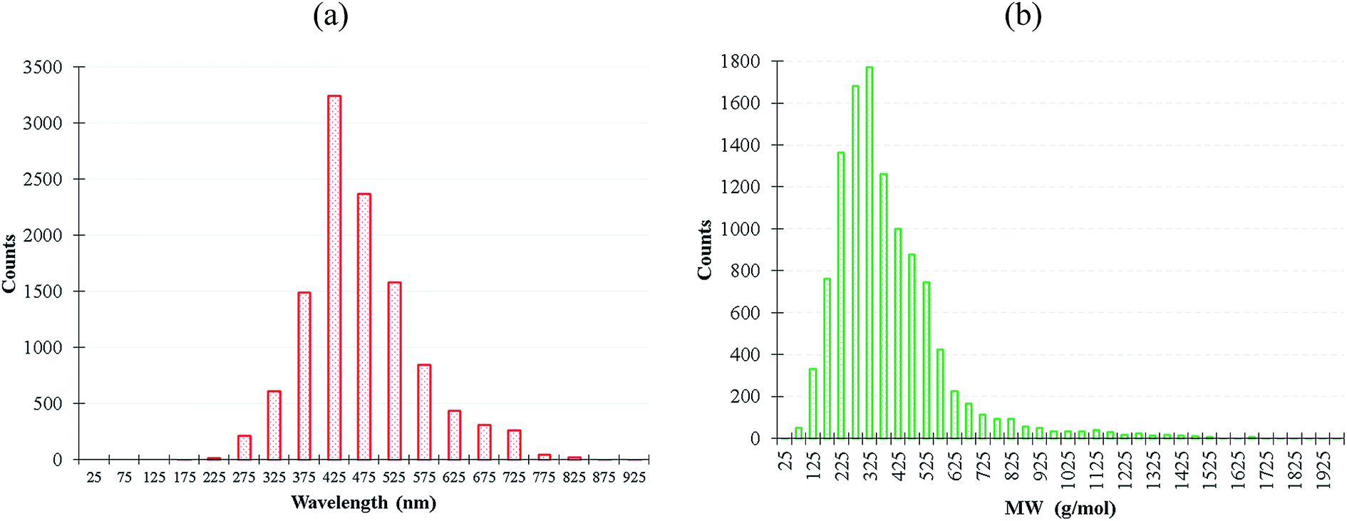Fig. 1 (a) Emission wavelength and (b) molecular weight distribution of the 11 460 fluorescent molecules.

Descriptor generation

We used PaDEL package²⁴ to generate two dimensional molecular descriptors and fingerprints for each fluorescent organic molecule, and the initial number of descriptors per molecule was 11 141. The complete list of the seventy categories of the generated descriptors from PaDEL is summarized in Table S1.†

Result and discussion

Descriptor dimension reduction

We first applied the variance threshold selection (VTS) to reduce the descriptor dimension where the descriptor with the variance σ² < 0.01 was removed. Consequently, the descriptor dimension was reduced from 11 411 to 6208, and most of the removed cases were fingerprint descriptors. We subsequently conducted the multiple linear regressions (MLR) with the 6208 descriptors, and denoted the results as VTS-MLR model.

Additionally, we built two more MLR based models for the comparison purpose. The first one used 4300 out of 6208 descriptors denoted as VTSsel-MLR model, where the dominant 4300 descriptors (|coefficient| > 5) determined by VTS-MLR model were taken into account. The second one contained only the 5158 fingerprint descriptors out of the VTS descriptor ensemble (the rest of the 1050 features are 2D descriptors), being denoted as VTSfp-MLR model.

The predicted results using VTS series MLR models are shown in Fig. 2 in comparison with the experiments. The R² values of these MLR models are summarized in Table 1 with all cases giving R² > 0.86. In order to examine the overfitting problem, we divided the descriptor dimension into 10 equivalent partitions and conducted cross validation to calculate the mean of 10-fold-R² (denoted as Q²) as shown in Table 1 (see Table S2† for the details of R² for each partition). The Q² results indicate that all three MLR models are found to be short of predictability and are not generalized. We believed that the failure of Q² results is due to the diverse characteristic of our collected dataset.

Fig. 2 The 2D histograms of the prediction vs. experiment comparison using the VTS series MLR models.

Table 1 The statistical properties of the VTS series MLR models

Models	# of descriptors	R^2	AdjR^2 ^a	Q^2
a AdjR^2 denotes the adjusted R^2 in respect to the size of the descriptor ensemble.
VTS-MLR	6208	0.92	0.66	−5143.72
VTSsel-MLR	4300	0.86	0.72	−49790.45
VTSfp-MLR	5158	0.89	0.62	−5.64 × 10^15

---

Descriptor dimension classification by Kmeans clustering

In order to gain better insights into the descriptor space, we conducted K-means clustering, an unsupervised machine learning method,²⁵ for classifying the VTS series descriptor ensembles. We first applied principle component analysis (PCA) method to convert the VTS (6208), VTSsel (4300), and VTSfp (5158) descriptor ensembles, respectively, into a finite 3 dimensional space. Subsequently, we used the three effective descriptors for K-means clustering²⁶ in order to identify the optimal number of sub-groups categorizing the 11 460 fluorescence molecules. The predicted inertia and Silhouette scores of k = 2–100 group partitions are shown in Fig. 3 (see ESI† for the details of both scoring functions). The Silhouette score of PCA-transformed VTS ensemble labeled as PCA-VTS (Fig. 3b) is found to be substantially different from other counterparts while no apparent elbow points could be identified form three inertia score curves. The highest Silhouette score at k = 15 suggests that the whole 11 460 molecules maybe reasonably categorized by 15 groups using PCA-VTS descriptor ensemble. In Fig. S1,† we also conducted the non-PCA transformed cases using VTS ensemble, and the corresponding results suggested PCA transformation was not trivial for classifying these complicated descriptor ensembles.

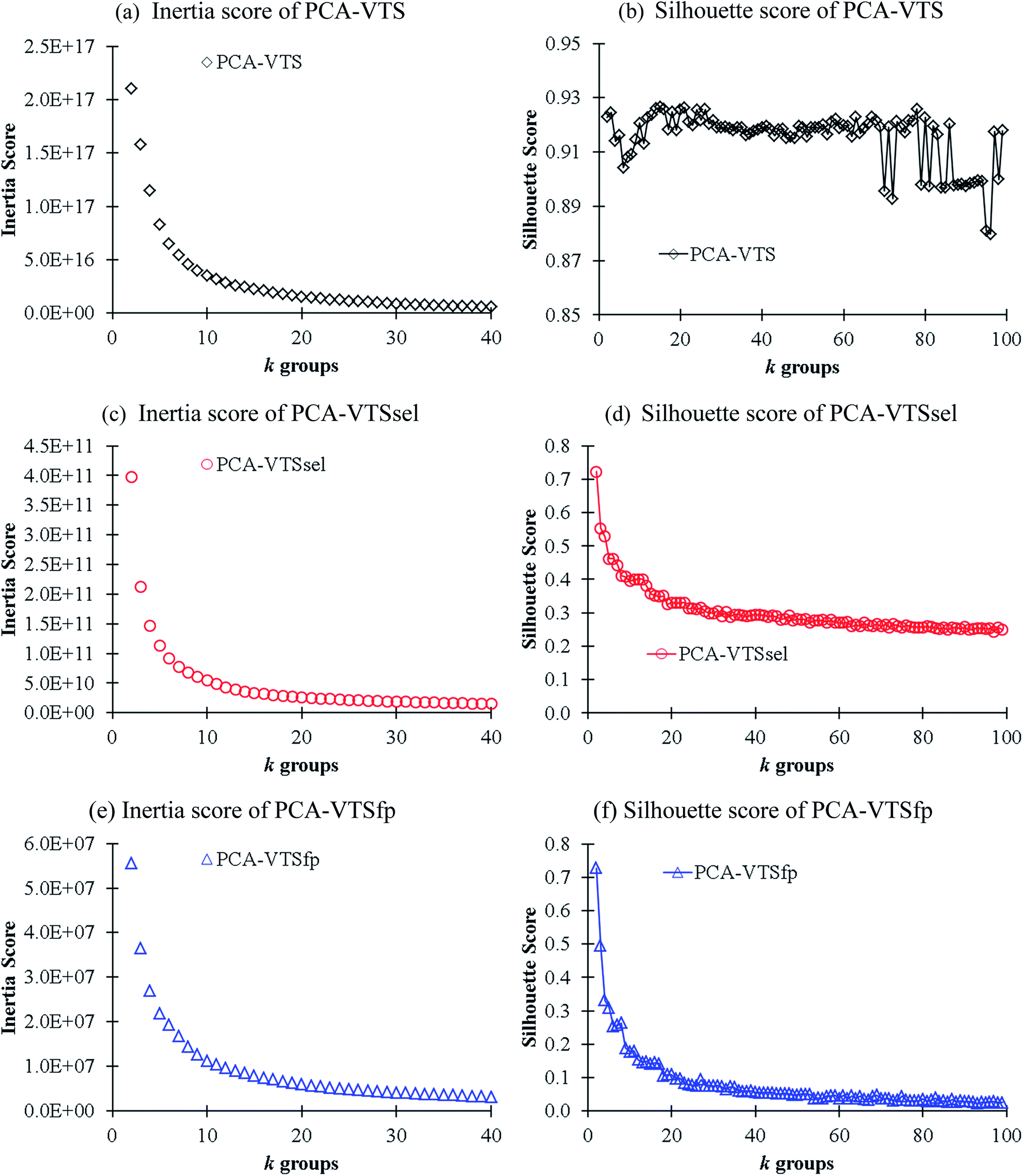Fig. 3 The calculated inertial (a, c and e) and Silhouette (b, d and f) scores in respect to k groups in K-means clustering analysis using the PCA-transformed descriptors of the VTS series ensembles.

With introducing K-means clustering, we intended to identify the general, however subtle, structural characteristics to categorize the collected fluorescent molecules. The visualization of the 15 sub-groups of 11 460 molecules using the PCA-transformed VTS, VTSsel, and VTSfp ensembles are projected onto the ternary plots in Fig. 4 (see Fig. S2† for the corresponding 3-dimentional plots) where the data distribution of the VTS ensemble (Fig. 4a) appeared to be the relatively distinguishable but not the optimal case.

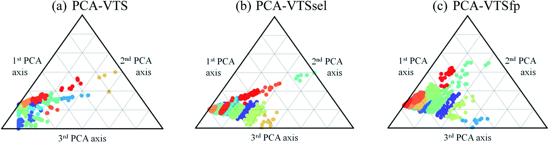Fig. 4 Three ternary plots of the 15 subgroups using the PCA-transformed descriptors for the VTS series ensembles. The 15 types of colors dots denote the subgroup distributions subject to the three PCA-transformed axes.

Extracting the dominant descriptors of each sub-group by Lasso regression

Lasso regression²⁷ was applied to extract the important descriptors for each subgroup (15 subgroups) of VTS ensemble. In according to the Lasso predicted contribution, we finally reduced the VTS ensemble from 6208 to 480 descriptors, denoted as Lasso ensemble, after collecting the filtered descriptor for each subgroup. The elbow curve of the inertia score of Lasso ensemble could be identified at k = 7 (see Fig. 5a and ESI†) while the comparable Silhouette scores predicted the acceptable grouping up to k = 13 (see Fig. 5b). The PCA-transformed ternary plots using k = 7 or 13 are shown in Fig. 5c and d, respectively (see Fig. S3† for the corresponding 3-dimensional plots). All of the color dots appeared to be well separated for both case, and suggests the 480 descriptor (Lasso) ensemble could well represent the overall structural characteristics. We, therefore, conducted the linear regression and nonlinear random forest regression²⁸ for the emission wavelength prediction using Lasso ensemble. A statistical performance comparison for the VTS series and Lasso models were provided in Table S3† based upon R², AdjR², Akaike's information criterion (AIC),²⁹ p-value and mean absolute error (MAE) against the experiments.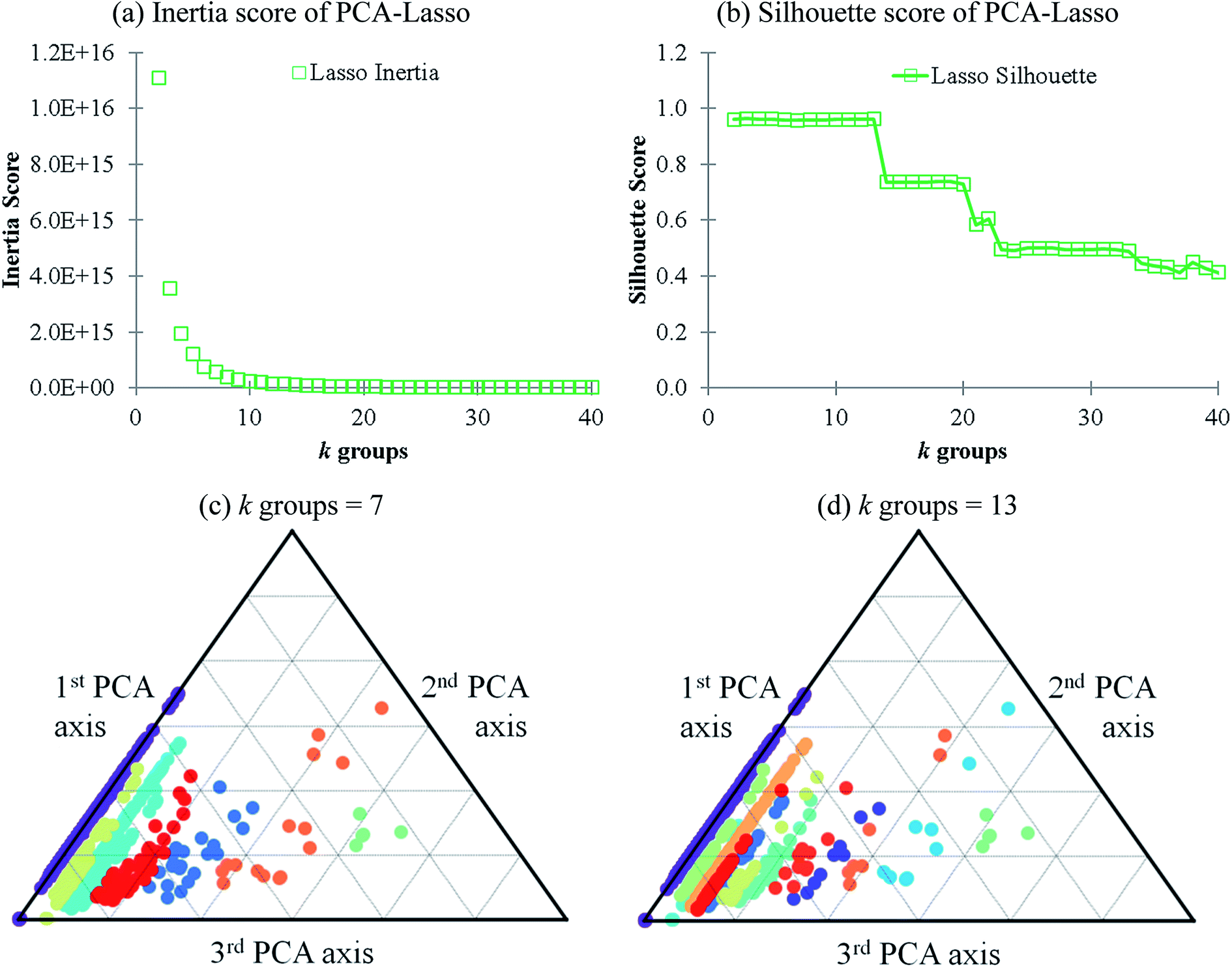

Fig. 5 (a and b) The inertia and Silhouette scores of Lasso ensemble, respectively; (c and d) the visualization of 7 and 13 groups of PCM-transformed 3-dimentional plot of Lasso ensemble, respectively.

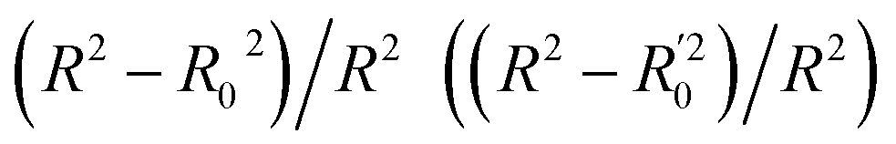
Golbraikh and Tropshas³⁰ suggested a combination of statistical criteria for demonstrating a statistically meaningful regression results as shown in Table 2. The ideal values for these statistical criteria are also summarized in Table 2 with k₀ denoting the linearity of predicted over experiment through the origin, and (R² − R₀²)/R² representing the predictive ability of the regression if the corresponding value <0.1. Both Lasso-LR and Lasso-RF models gave reasonable predictability with MAE at 40 and 24 nm, respectively, and the transferability of these models also appeared to be significantly better than the VTS series models (see Q² values in Tables 2 and S2†). Despite the Lasso-RF model gave better predictability than the LR counterpart, the LR model still provided qualitative results in addition to its interpretability (Fig. 6).

Table 2 The statistical benchmark of Lasso-LR and Lasso-RF models

Criterion	R^2^a	Rtest^2 (MAE)^a	Q^2	^b	^c	^c
a Only 80% of 11 460 samples were selected (randomly) as the training set for the Lasso-LR and Lasso-RF models. The rest of 20% samples were used as the testing set with MAE (in nm) shown in the parentheses.b The value of k0 denotes the slope of the predicted over experimental data through the origin (intercept equal to zero), and is the inverse k0. The detailed information is summarized in ESI.c R0^2 denotes the correlation coefficient of k0, and denotes the case of . See ESI for more details.
Ideal values	>0.6	>0.6	>0.5	0.85 ≤ k ≤ 1.15 (0.85 ≤ k′ ≤ 1.15)	Close to R^2 (close to R^2)	<0.1 (<0.1)
Lasso-LR	0.6632	0.5685 (44)	0.5800	0.9868 (0.9999)	0.6627 (0.4984)	0.0009 (0.2486)
Lasso-RF	0.9227	0.7004 (36)	0.6205	0.9919 (1.0025)	0.8565 (0.7933)	0.0717 (0.1402)

---

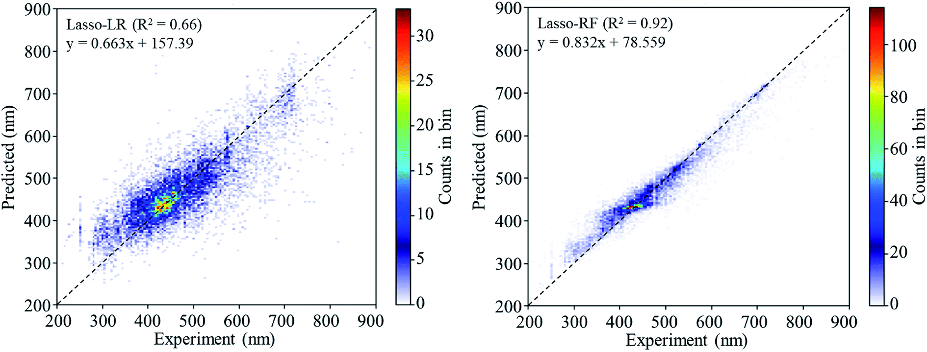Fig. 6 The 2D histograms of the regression results of Lasso-LR and Lasso-RF models. The legend shows the linear equation fitting to the predicted values.

Comparison of informatics vs. quantum mechanics approaches

We selected 20 fluorescence compounds rom Reaxys in addition to the original 11 460 samples, 5 compounds per 100 nm interval between 300–700 nm for carrying out the emission wavelength predictions using time-dependent density functional theory calculations, one of the common methods in predicting emission wavelength using QM approach (see Table S4† for the corresponding SMILES). We employed wB97XD functional³¹ and 6-31+G(d) basis set under the implicit solvation model (PCM of ethanol) with Gassian16 package³² for the S1 state optimization. The emission wavelength was further calibrated by the vertical S0 to S1 excitation energy computed at wB97XD/6-311+G(d,p) level using the prior minimum structure of S1 state. In Fig. 7 and Table S4,† the Lasso-RF model appears to give the reasonable R² value (R² = 0.655, MEA = 48 nm) in comparison against the selected DFT predictions (R² = 0.778, MAE = 60 nm) with significantly less computational expense. The Lasso-RF approach is consequently recommended for the large scale and high-throughput screenings on the emission wavelength of the organic fluorophores being complementary to the TDDFT calculations.

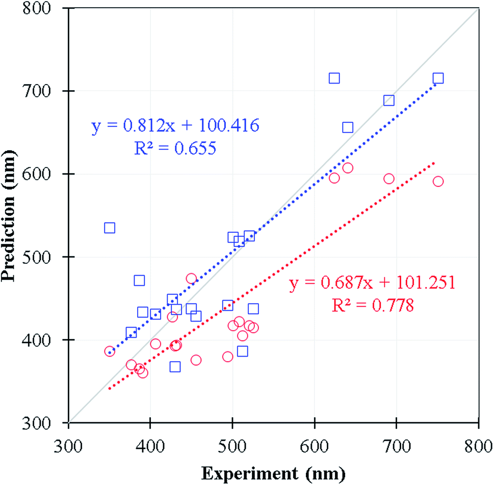Fig. 7 The comparison of the predicted wavelength in nm of DFT (red) and Lasso-RF (blue) models. The linear equations of both predicted data are shown in dotted lines. The grey solid line denotes the ideal fitting of slope = 1.

Important descriptors extracted from Lasso-RF model

We applied an assemble method like random forest where the descriptor importance could be estimated by calculating the decrease in node impurity weighted by the probability of reaching the node. The node probability could be calculated by the number of samples reaching the node, divided by the total number of samples. The current Lasso-RF model is schematically shown in Fig. S4.† The dominant descriptors of Lasso-RF model are summarized in Fig. 8 where the nTG12Ring and nTG12HeteroRing descriptors describing the number of >12-membered homogeneous and heterogeneous rings are the leading two contributions, followed by SubFPC287 for counting the number of conjugated double bonds and nAtomP denoting the number of atoms in the largest π system. All of the leading four descriptors can be used in conjunction with the conventional QM viewpoint that higher degree of conjugated π-bonding patterns shall introduce smaller HOMO–LUMO gaps and lead to the longer fluorescence emission wavelength.

Fig. 8 Top 20 important descriptors predicted by the Lasso-RF model.

Conclusion

In this study, we imported ten-thousand-plus organic fluorophore as the sample dataset and conducted a clustering and machine learning approach using molecular descriptors for predicting the emission wavelength. We demonstrated a systematic procedure in reducing the descriptor dimension in terms of the measurements of several statistical indicators. We finally concluded with the Lasso-RF model for the numerically predicted wavelength as well as being fulfilled with the statistical criteria. The model identified four conjugated π-bonding related descriptors to dominantly contribute to the predicted emission wavelength. Such an informatics model appeared to bring comparable predictive ability in complementary to the conventional time-dependent density functional theory method in emission wavelength prediction, however, with a fractional computational expense.

Conflicts of interest

There are no conflicts to declare.

Acknowledgements

This study is supported by the Ministry of Science and Technology of Taiwan (108-2113-M-003-003) and the Innovation-Oriented Trilateral Research Fund for Young Investigators of NTU system. The authors acknowledge the preliminary explorations by Mr Yi-Ming Chou and Shao-Ting Luo. The authors are grateful for the computational resources provided by the National Center for High-Performance Computing of Taiwan and the Center for Cloud Computing in National Taiwan Normal University.

References

1. E. A. Specht, E. Braselmann and A. E. Palmer, Annu. Rev. Physiol., 2017, 79, 93–117.
2. Z. He, C. Ke and B. Z. Tang, ACS Omega, 2018, 3, 3267–3277.
3. E. Kim and S. B. Park, in Advanced Fluorescence Reporters in Chemistry and Biology, Springer, Berlin Heidelberg, 2010, pp. 149–186.
4. M. Sauer, J. Hofkens and J. Enderlein, Handbook of Fluorescence Spectroscopy and Imaging: From Single Molecules to Ensembles, WileyVCH, Weinheim, 2011.
5. J. Liu, C. Liu and W. He, Curr. Org. Chem., 2013, 17, 564–579.
6. A. Vogel, Ann. Phys., 1820, 64, 161–166.
7. J. Chen, W. Liu, J. Ma, H. Xu, J. Wu, X. Tang, Z. Fan and P. Wang, J. Org. Chem., 2012, 77, 3475–3482.
8. A. F. A. Cros, Action de l'alcool amylique sur l'organisme, Faculté de médecine de Strasbourg, Strasbourg, 1863.
9. R. Todeschini and V. Consonni, Handbook of Molecular Descriptors, WileyVCH, Weinheim, 2000.
10. S. M. Weiss and C. A. Kulikowski, Computer Systems that Learn: Classification and Prediction Methods from Statistics, Neural Nets, Machine Learning, and Expert Systems, Morgan Kaufmann Publishers Inc., Burlington, 1991.
11. R. D. King, J. D. Hirst and M. J. E. Sternberg, Perspect. Drug Discovery Des., 1993, 1, 279–290.
12. J.-N. Wang, J.-L. Jin, Y. Geng, S.-L. Sun, H.-L. Xu, Y.-H. Lu and Z.-M. Su, J. Comput. Chem., 2013, 34, 566–575.
13. H. Li, Z. Zhong, L. Li, R. Gao, J. Cui, T. Gao, L. H. Hu, Y. Lu, Z. M. Su and H. Li, J. Comput. Chem., 2015, 36, 1036–1046.
14. R. S. da Silva, L. F. Marins, D. V. Almeida, K. dos Santos Machado and A. V. Werhli, Comput. Biol. Chem., 2019, 83, 107089.
15. R. Gómez-Bombarelli, J. N. Wei, D. Duvenaud, J. M. Hernández-Lobato, B. Sánchez-Lengeling, D. Sheberla, J. Aguilera-Iparraguirre, T. D. Hirzel, R. P. Adams and A. Aspuru-Guzik, ACS Cent. Sci., 2018, 4, 268–276.
16. J. Noh, J. Kim, H. S. Stein, B. Sanchez-Lengeling, J. M. Gregoire, A. Aspuru-Guzik and Y. Jung, Matter, 2019, 1, 1370–1384.
17. L. Himanen, M. O. J. Jäger, E. V. Morooka, F. Federici Canova, Y. S. Ranawat, D. Z. Gao, P. Rinke and A. S. Foster, Comput. Phys. Commun., 2020, 247, 106949.
18. K. Rossi and J. Cumby, Int. J. Quantum Chem., 2020, 120, e26151.
19. M. F. Langer, A. Goeßmann and M. Rupp, 2020, arXiv:2003.12081.
20. M. Rupp, A. Tkatchenko, K.-R. Müller and O. A. von Lilienfeld, Phys. Rev. Lett., 2012, 108, 058301.
21. E. O. Pyzer-Knapp, K. Li and A. Aspuru-Guzik, Adv. Funct. Mater., 2015, 25, 6495–6502.
22. K. Ghosh, A. Stuke, M. Todorović, P. B. Jørgensen, M. N. Schmidt, A. Vehtari and P. Rinke, Adv. Sci., 2019, 6, 1970053.
23. Reaxys, http://www.reaxys.com/, accessed on June 1, 2018.
24. C. W. Yap, J. Comput. Chem., 2011, 32, 1466–1474.
25. S. Lloyd, IEEE Trans. Pattern Anal. Mach. Intell., 1982, 28, 129–137.
26. C. Ding and X. He, presented in part at the proceedings of the twenty-first international conference on machine learning, Banff, Alberta, Canada, 2004.
27. R. Tibshirani, J. Roy. Stat. Soc. B Stat. Methodol., 2011, 73, 273–282.
28. H. Tin Kam, IEEE Trans. Pattern Anal. Mach. Intell., 1998, 20, 832–844.
29. H. Akaike, IEEE Trans. Autom. Control, 1974, 19, 716–723.
30. A. Golbraikh and A. Tropsha, J. Mol. Graphics Modell., 2002, 20, 269–276.
31. J.-D. Chai and M. Head-Gordon, Phys. Chem. Chem. Phys., 2008, 10, 6615–6620.
32. M. J. Frisch, G. W. Trucks, H. B. Schlegel, G. E. Scuseria, M. A. Robb, J. R. Cheeseman, G. Scalmani, V. Barone, G. A. Petersson, H. Nakatsuji, X. Li, M. Caricato, A. V. Marenich, J. Bloino, B. G. Janesko, R. Gomperts, B. Mennucci, H. P. Hratchian, J. V. Ortiz, A. F. Izmaylov, J. L. Sonnenberg, D. Williams-Young, F. Ding, F. Lipparini, F. Egidi, J. Goings, B. Peng, A. Petrone, T. Henderson, D. Ranasinghe, V. G. Zakrzewski, J. Gao, N. Rega, G. Zheng, W. Liang, M. Hada, M. Ehara, K. Toyota, R. Fukuda, J. Hasegawa, M. Ishida, T. Nakajima, Y. Honda, O. Kitao, H. Nakai, T. Vreven, K. Throssell, J. A. Montgomery Jr, J. E. Peralta, F. Ogliaro, M. J. Bearpark, J. J. Heyd, E. N. Brothers, K. N. Kudin, V. N. Staroverov, T. A. Keith, R. Kobayashi, J. Normand, K. Raghavachari, A. P. Rendell, J. C. Burant, S. S. Iyengar, J. Tomasi, M. Cossi, J. M. Millam, M. Klene, C. Adamo, R. Cammi, J. W. Ochterski, R. L. Martin, K. Morokuma, O. Farkas, J. B. Foresman and D. J. Fox, Gaussian, Inc., Wallingford CT, 2016.
33. F. Häse, C. Kreisbeck and A. Aspuru-Guzik, Machine learning for quantum dynamics: deep learning of excitation energy transfer properties, Chem. Sci., 2017, 8, 8419–8426.

---

Footnote

† Electronic supplementary information (ESI) available: All of the descriptor categories from PaDEL, the selected compounds for DFT vs. Lasso-RF comparison, the schematic representation of Lasso-RF model. See DOI: 10.1039/d0ra05014h

---