DOI:
10.1039/D0RA03031G
(Paper)
RSC Adv., 2020,
10, 20646-20653
Relative cooling power modeling of lanthanum manganites using Gaussian process regression
Received
3rd April 2020
, Accepted 24th May 2020
First published on 1st June 2020
Abstract
Efficient solid-state refrigeration techniques at room temperature have drawn increasing attention due to their potential for improving energy efficiency of refrigeration, air-conditioning, and temperature-control systems without using harmful gas in conventional gas compression techniques. Recent developments of increased magnetocaloric effects and relative cooling power (RCP) in ferromagnetic lanthanum manganites show promising results of further developments in magnetic refrigeration devices. By incorporating chemical substitutions, oxygen content modifications, and various synthesis methods, these manganites experience lattice distortions from perovskite cubic structures to orthorhombic structures. Lattice distortions, revealed by changes in lattice parameters, have significant influences on adiabatic temperature changes and isothermal magnetic entropy changes, and thus RCP. Empirical results and previous models through thermodynamics and first-principles have shown that changes in lattice parameters correlate with those in RCP, but correlations are merely general tendencies and obviously not universal. In this work, the Gaussian process regression model is developed to find statistical correlations and predict RCP based on lattice parameters among lanthanum manganites. This modeling approach demonstrates a high degree of accuracy and stability, contributing to efficient and low-cost estimations of RCP and understandings of magnetic phase transformations and magnetocaloric effects in lanthanum manganites.
1 Introduction
Energy efficiency and sustainability are priority topics in modern society. Refrigeration and air conditioning account for a significant amount of power consumption among various end uses of energy in both commercial and residential areas.10 Most refrigeration technology relies on the conventional gas compression (CGC) technique, which has drawn increasing criticisms due to its lack of efficiency and use of air-pollutant gas. Recent developments of magnetic refrigeration (MR) technology, based on the magnetocaloric effect in magnetic materials particularly near room temperature, have offered an exciting alternative to vapor compression refrigeration.20 Advantages of MR technology over CGC include, but not limited to, almost ten-fold higher cooling efficiency in magnetic refrigerators, much smaller footprints, complete solid-state operation, and being environmentally friendly.21 Furthermore, recent developments in high-temperature superconductors with enhanced critical temperature and magnetic fields that can be generated have prompted developments of high-efficiency MR devices with superconducting magnetic field sources.8,22,28–30 An early development of a gadolinium (Gd) rare earth metal with a large magnetocaloric effect (MCE) marked a significant starting point in developing room-temperature MR, but its application in large-scale commercial usage was greatly limited due to the very high price of Gd.9 Therefore, numerous research has been conducted to search for new materials with large MCEs, large relative cooling power (RCP), and cheap prices.
Among these materials, ferromagnetic lanthanum manganites, with the general formula, La1−x−yRExAyMn1−zTMzO3 where RE is a rare earth element that partially or totally substitutes lanthanum, A is an element of the IA or IIA group, and TM is a transition element that partially substitutes Mn, are of practical importance. These materials have unique properties such as small magnetic and thermal hysteresis, a large MCE around Curie temperature TC, and a broad working temperature range. Furthermore, manganites are inexpensive to prepare, chemically stable, and highly electrically resistive.6 The parent LaMnO3 compound is semiconducting and orders antiferromagnetically at 150 K, but a formation of mixed valence in Mn ions via a double exchange mechanism between Mn4+ and Mn3+ can induce ferromagnetism. A wide range of TC from ∼150 K to 375 K can be obtained by, for example, substitution of a divalent ion (Ca2+, Ba2+, Sr2+, etc.) or a monovalent ion (Na1+, K1+, etc.) for La3+, and an excess of oxygen. Furthermore, the ground state of manganites can be tuned by partial substitution of La3+ by a trivalent rare earth, or in a La-free Pr or Nd manganites. These perovskite-based structures show lattice distortions as a result of modifications from the cubic structure by the deformation of the MnO6 octahedron arising from the Jahn–Teller effect and/or changes in the connective pattern of the MnO6 octahedra in the perovskite structure.26,27 Values of TC, magnetic entropy changes ΔSm, adiabatic temperature changes ΔTad, and the resultant RCP are strongly dependent on the doping mechanisms and thus lattice distortions.
Qualitative analysis on the effect of dopant types and levels on RCP of lanthanum manganites has been conducted through experiments, mainly by varying synthesis methods (solid-state reaction, wet chemistry, sol–gel, etc.), morphologies (particle size, shape, etc.), crystalline states, and final forms (powder, pellet, film, etc.).1,3,4,11–14,16–18,23–25 Quantitative analysis through thermodynamics models and first-principle models has been utilized to aid the understanding of magnetothermal responses of these materials and facilitate the searching of new candidates for MR devices.2,5,7,15 However, these models require a significant amount of data inputs, such as variables for equations of state, exchange coupling energies, and magnetic moments of magnetocaloric materials, which can only be obtained by extensive measurements.
In this work, the Gaussian process regression (GPR) model is developed to elucidate the statistical relationship between RCP and lattice parameters of orthorhombic lanthanum manganites. The model generalizes well in the presence of only a few descriptive features, where intelligent algorithms are able to learn and recognize the patterns. This modeling approach demonstrates a high degree of accuracy and stability, contributing to efficient and low-cost estimations of RCP and understandings of which based on lattice parameters. As one of the computational intelligence techniques, the GPR model has already been utilized in other materials systems to predict significant physical parameters in different fields of applications.31–44 On one hand, the model can serve as a guideline for searching for doped-manganites with a large RCP value by screening the lattice parameters. On the other hand, the model can be used as part of machine learning to aid the understanding of the magnetic phase transformation in various types of doped-manganites.
The remaining of this work is organized as follows. Section 2 proposes the GPR model. Section 3 describes the data and computational methodology. Section 4 presents and discusses results, and Section 5 concludes.
2 Proposed methodology
2.1 Brief description of Gaussian process regression
GPRs are nonparametric kernel-based probabilistic models. Consider a training dataset, {(xi,yi); i = 1, 2, …, n} where  and
and  , from an unknown distribution. A trained GPR predicts values of the response variable ynew given an input matrix xnew.
Recall a linear regression model, y = xTβ + ε, where ε ∼ N(0,σ2). A GPR aims at explaining y by introducing latent variables, l(xi) where i = 1, 2, …, n, from a Gaussian process such that the joint distribution of l(xi)'s is Gaussian, and explicit basis functions, b. The covariance function of l(xi)'s captures the smoothness of y and basis functions project x into a feature space of dimension p.
A GP is defined by the mean and covariance. Let m(x) = E(l(x)) be the mean function and k(x,x′) = Cov[l(x),l(x′)] the covariance function, and consider now the GPR model, y = b(x)Tβ + l(x), where l(x) ∼ GP(0,k(x,x′)) and  . k(x,x′) is often parameterized by the hyperparameter, θ, and thus might be written as k(x,x′|θ). In general, different algorithms estimate β, σ2, and θ for model training and would allow specifications of b and k, as well as initial values for parameters.
The current study explores four kernel functions, namely exponential, squared exponential, Matern 5/2, and rational quadratic, whose specifications are listed in eqn (1)–(4), respectively, where σl is the characteristic length scale defining how far apart x's can be for y's to become uncorrelated, σf is the signal standard deviation,  , and α is a positive-valued scale-mixture parameter. Note that σl and σf should be positive. This could be enforced through θ such that θ1 = log
![[thin space (1/6-em)]](https://www.rsc.org/images/entities/char_2009.gif) σl and θ2 = log
σl and θ2 = log![[thin space (1/6-em)]](https://www.rsc.org/images/entities/char_2009.gif) σf.
σf.
| |
 | (1) |
| |
 | (2) |
| |
 | (3) |
| |
 | (4) |
Similarly, three basis functions are investigated here, namely constant, linear, and pure quadratic, whose specifications are listed in eqn (5)–(7), respectively, where B = (b(x1), b(x2), …, b(xn))T, X = (x1, x2, …, xn)T, and 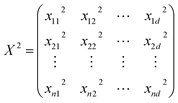 .
.
To estimate the GPR model, a Bayesian optimization algorithm is utilized. With a Gaussian process model of f(x), the algorithm evaluates yi = f(xi) for Ns points xi taken at random within the variable bounds, where Ns points stand for the number of initial evaluation points and 4 is used. If there are evaluation errors, it takes more random points until Ns successful evaluations are arrived-at. The algorithm then repeats the following two steps: (1) updating the Gaussian process model of f(x) to obtain a posterior distribution over functions Q(f|xi,yi for i = 1, … ,n); (2) finding the new point x that maximizes the acquisition function a(x). It stops after reaching 30 iterations. The acquisition function, a(x), evaluates the goodness of a point, x, based on the posterior distribution function, Q. This work employs the lower-confidence-bound (LCB) acquisition function, which looks at the curve G two standard deviations, σQ, below the posterior mean, μQ, at each point: G(x) = μQ(x) − 2σQ(x). Therefore, G(x) is the 2σQ lower confidence envelope of the objective function model. The algorithm then maximizes the negative of G: LCB = 2σQ(x) − μQ(x). The optimization is carried out on σ, the noise standard deviation. θ and β are estimated by maximizing the log likelihood function.
2.2 Performance evaluation
Performance of the proposed GPR models is evaluated using the root mean square error (RMSE), mean absolute error (MAE), and correlation coefficient (CC) in eqn (8), (9), and (10) respectively, where n is the number of data points, Texpi and Testi are the i-th (i = 1, 2, …, n) experimental and estimated magnetic cooling power, and  and
and  are their averages.
| |
 | (8) |
| |
 | (9) |
| |
 | (10) |
3 Empirical study
3.1 Description of dataset
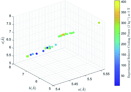
The experimental data used, shown in Table 1 (Columns 1–5), are obtained from ref. 1, 3, 4, 11–14, 16–18 and 23–25, most of which have been modeled through the support vector machine regression model.19 The dataset covers a wide range of doped lanthanum manganites in the form of bulk polycrystalline, single crystal, powders, and sintered pellets, by different synthesis routes including the solid-state reaction, wet-mix processing, and sol–gel processing. RCP values are calculated from ΔSm and the full width at half maximum (FWHM) of the ΔSm vs. T curve under Δ(μ0H) of 5 T. Data visualization in Fig. 1 reveals nonlinear relationships, which are modeled through the GPR.
Table 1 Experimental data and relative cooling power predictionsa
| Sample |
a (Å) |
b (Å) |
c (Å) |
Experimental relative cooling power (J kg−1) |
Predicted relative cooling power (J kg−1) |
Reference |
Magnetic property |
| “a (Å),” “b (Å),” and “c (Å)” are lattice parameters. “Predicted relative cooling power (J kg−1)” shows the result from the current work, meaning predicted values based on the Gaussian process regression. “Experimental relative cooling power (J kg−1)” and “Predicted relative cooling power (J kg−1)” are visualized in Fig. 2. “□” in sample names stands for “vacancy.” “FM” means “ferromagnetism,” “AFM” means “anti-ferromagnetism,” and “PM” means “paramagnetism”. |
| La0.8Ca0.2MnO3 |
5.4972 |
7.7771 |
5.5149 |
3.67 |
3.70 |
13 |
2nd order FM–PM transition |
| Pr0.7Ca0.3MnO3 |
5.4598 |
7.6741 |
5.4303 |
9.72 |
9.87 |
25 |
2nd order FM–PM transition |
| Pr0.7Ca0.3MnO3 |
5.4598 |
7.6741 |
5.4303 |
10.00 |
9.87 |
4 |
2nd order FM–PM transition |
| La0.6Pr0.1Ba0.3Mn0.7Ni0.3O3 |
5.4813 |
7.6853 |
5.4519 |
62.00 |
62.02 |
18 |
2nd order FM–PM transition |
| La0.67Ca0.33Mn0.75Cr0.25O3 |
5.4419 |
7.6921 |
5.4608 |
88.00 |
88.02 |
17 |
2nd order FM–PM transition |
| La0.6Pr0.1Ba0.3Mn0.9Ni0.1O3 |
5.5032 |
7.7200 |
5.4690 |
123.00 |
123.01 |
18 |
2nd order FM–PM transition |
| La0.67Ca0.33Mn0.9Cr0.1O3 |
5.4486 |
7.7000 |
5.4673 |
147.00 |
147.01 |
17 |
2nd order FM–PM transition |
| La0.8Ca0.05□0.15MnO3 |
5.5253 |
7.8002 |
5.5152 |
175.00 |
175.01 |
13 |
2nd order FM–PM transition |
| La0.8Ca0.1□0.1MnO3 |
5.5050 |
7.7866 |
5.5255 |
179.00 |
179.01 |
13 |
2nd order FM–PM transition |
| La0.8Ca0.15□0.05MnO3 |
5.5066 |
7.7937 |
5.5084 |
183.00 |
183.01 |
13 |
2nd order FM–PM transition |
| Pr0.7Ca0.3Mn0.9Fe0.1O3 |
5.4319 |
7.6753 |
5.4646 |
183.50 |
183.52 |
23 |
2nd order FM–PM transition |
| Pr0.6Ca0.1Sr0.3Mn0.975Fe0.025O3 |
5.4384 |
5.4624 |
7.6776 |
192.00 |
192.01 |
14 |
2nd order FM–PM transition |
| Pr0.2Sm0.35Sr0.45MnO3 |
5.4533 |
5.4380 |
7.6786 |
219.03 |
219.03 |
16 |
1st order (AFM, FM)–PM transition |
| Pr0.7Ca0.3Mn0.9Cr0.1O3 |
5.4293 |
7.6691 |
5.4552 |
222.78 |
246.39 |
23 |
2nd order FM–PM transition |
| La0.5Sm0.2Sr0.3Mn0.85Fe0.15O3 |
5.5038 |
7.7388 |
5.4746 |
226.00 |
226.00 |
1 |
2nd order FM–PM transition |
| La0.6Pr0.1Ba0.3MnO3 |
5.5121 |
7.7508 |
5.4859 |
230.00 |
230.00 |
18 |
2nd order FM–PM transition |
| Pr0.3Sm0.25Sr0.45MnO3 |
5.4623 |
5.4387 |
7.6779 |
230.01 |
230.01 |
16 |
1st order (AFM, FM)–PM transition |
| Pr0.6Ca0.1Sr0.3Mn0.95Fe0.05O3 |
5.4382 |
5.4632 |
7.6826 |
233.00 |
233.00 |
14 |
2nd order FM–PM transition |
| Pr0.4Sm0.15Sr0.45MnO3 |
5.4718 |
5.4399 |
7.6773 |
240.00 |
240.00 |
16 |
1st order (AFM, FM)–PM transition |
| Pr0.5K0.05Sr0.45MnO3 |
5.4825 |
5.4429 |
7.6503 |
241.20 |
241.20 |
12 |
2nd order FM–PM transition |
| Nd0.67Ba0.33Mn0.98Fe0.02O3 |
5.4917 |
7.7602 |
5.5196 |
242.00 |
242.00 |
11 |
2nd order FM–PM transition |
| Pr0.6Ca0.1Sr0.3MnO3 |
5.4375 |
5.4647 |
7.6814 |
243.00 |
243.00 |
14 |
2nd order FM–PM transition |
| Pr0.6Ca0.1Sr0.3Mn0.925Fe0.075O3 |
5.4427 |
5.4669 |
7.6919 |
256.00 |
256.00 |
14 |
2nd order FM–PM transition |
| Pr0.1Sm0.45Sr0.45MnO3 |
5.4427 |
5.4415 |
7.6800 |
258.82 |
258.82 |
16 |
1st order (AFM, FM)–PM transition |
| Nd0.67Ba0.33MnO3 |
5.4915 |
7.7591 |
5.5519 |
265.00 |
265.00 |
11 |
2nd order FM–PM transition |
| Pr0.5Na0.05Sr0.45MnO3 |
5.4772 |
5.4420 |
7.6441 |
266.20 |
266.20 |
12 |
2nd order FM–PM transition |
| La0.5Sm0.2Sr0.3MnO3 |
5.5019 |
7.7321 |
5.4696 |
268.00 |
268.00 |
1 |
2nd order FM–PM transition |
| Pr0.7Ca0.3Mn0.98Co0.02O3 |
5.4303 |
7.6729 |
5.4599 |
268.14 |
268.14 |
25 |
2nd order FM–PM transition |
| Pr0.7Ca0.3Mn0.9Cr0.1O3 |
5.4293 |
7.6691 |
5.4552 |
270.00 |
246.39 |
4 |
1st order FM–PM transition |
| La0.5Sm0.2Sr0.3Mn0.95Fe0.05O3 |
5.5036 |
7.7252 |
5.4678 |
280.00 |
279.99 |
1 |
2nd order FM–PM transition |
| La0.5Sm0.2Sr0.3Mn0.9Fe0.1O3 |
5.5027 |
7.7403 |
5.4740 |
285.00 |
284.99 |
1 |
2nd order FM–PM transition |
| Pr0.8Na0.1K0.1MnO3 |
5.4578 |
5.4588 |
7.7263 |
292.24 |
292.23 |
3 |
2nd order FM–PM transition |
| Pr0.8Na0.05K0.15MnO3 |
5.5641 |
5.4661 |
7.7374 |
293.21 |
293.20 |
3 |
2nd order FM–PM transition |
| Pr0.7Ca0.3Mn0.9Co0.1O3 |
5.4306 |
7.6705 |
5.4484 |
300.80 |
300.80 |
23 |
2nd order FM–PM transition |
| Pr0.7Ca0.3Mn0.9Co0.1O3 |
5.4306 |
7.6705 |
5.4484 |
300.80 |
300.80 |
25 |
2nd order FM–PM transition |
| Pr0.7Ca0.3Mn0.9Ni0.1O3 |
5.4328 |
7.6892 |
5.4195 |
308.70 |
308.69 |
23 |
2nd order FM–PM transition |
| Pr0.8Na0.15K0.05MnO3 |
5.4507 |
5.4525 |
7.7165 |
325.98 |
325.97 |
3 |
1st order FM–PM transition |
| Pr0.7Ca0.3Mn0.95Fe0.05O3 |
5.4321 |
7.6743 |
5.4648 |
337.40 |
337.38 |
24 |
2nd order FM–PM transition |
| Pr0.7Ca0.3Mn0.95Ni0.05O3 |
5.4295 |
7.6708 |
5.4508 |
352.20 |
352.19 |
24 |
2nd order FM–PM transition |
| Pr0.8Na0.2MnO3 |
5.4460 |
5.4481 |
7.7113 |
355.62 |
355.61 |
3 |
1st order (AFM, FM)–PM transition |
| Pr0.7Ca0.3Mn0.95Co0.05O3 |
5.4299 |
7.6696 |
5.4572 |
378.20 |
378.20 |
24 |
2nd order FM–PM transition |
| Pr0.7Ca0.3Mn0.95Co0.05O3 |
5.4314 |
7.6711 |
5.4591 |
378.20 |
378.18 |
25 |
2nd order FM–PM transition |
| Pr0.7Ca0.3Mn0.95Cr0.05O3 |
5.4300 |
7.6679 |
5.4572 |
405.72 |
405.85 |
24 |
2nd order FM–PM transition |
| Pr0.7Ca0.3Mn0.95Cr0.05O3 |
5.4300 |
7.6679 |
5.4572 |
406.00 |
405.85 |
4 |
2nd order FM–PM transition |
| Mean |
5.4636 |
6.9903 |
6.1761 |
239.44 |
239.44 |
— |
— |
| Median |
5.4520 |
7.6710 |
5.4743 |
249.50 |
246.39 |
— |
— |
| Standard deviation |
0.0340 |
1.0638 |
1.0452 |
98.66 |
98.52 |
— |
— |
| Minimum |
5.4293 |
5.4380 |
5.4195 |
3.67 |
3.70 |
— |
— |
| Maximum |
5.5641 |
7.8002 |
7.7374 |
406.00 |
405.85 |
— |
— |
| Correlation coefficient with relative cooling power |
−30.47% |
−15.67% |
14.69% |
— |
99.87% |
— |
— |
 |
| | Fig. 1 Magnetic cooling power and lattice parameters, a (Å), b (Å), and c (Å). | |
3.2 Computational methodology
MATLAB is utilized for computations and simulations in this work. All observations are used to train the final GPR model given the relative small sample size. The stability of the GPR approach is confirmed by bootstrap analysis.
4 Result and discussion
4.1 Comparison with previous study
The final GPR model is detailed in Fig. 2, whose performance is compared with that based on the SVM regression in ref. 19.† Switching from the SVM to GPR, the CC increases from 85.07% to 99.87%, the RMSE decreases from 50.5315 to 5.0339, and the MAE decreases from 26.3802 to 1.0923. The GPR model thus provides more accurate relative cooling power predictions than the SVM regression. The result in Fig. 2 shows good alignment between GPR predicted and experimental data.
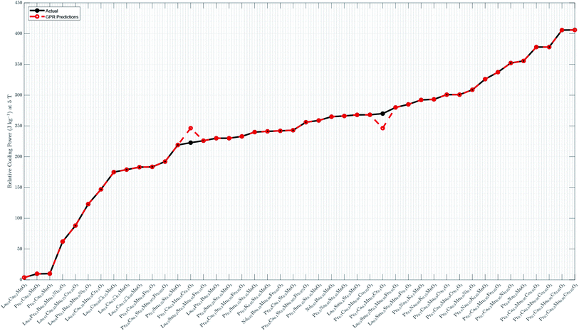 |
| | Fig. 2 Experimental vs. predicted relative cooling power. The GPR model is built using the whole sample with the Matern 5/2 kernel, constant basis function, and standardized lattice parameters. It has a log-likelihood of −813.7988, ![[small beta, Greek, circumflex]](https://www.rsc.org/images/entities/i_char_e114.gif) of 233.9604, of 233.9604, ![[small sigma, Greek, circumflex]](https://www.rsc.org/images/entities/i_char_e111.gif) of 0.9866, of 0.9866, ![[small sigma, Greek, circumflex]](https://www.rsc.org/images/entities/i_char_e111.gif) l of 0.0053, and l of 0.0053, and ![[small sigma, Greek, circumflex]](https://www.rsc.org/images/entities/i_char_e111.gif) f of 89.8778. Detailed numerical predictions are listed in Table 1 (Column 6). “□” in sample names stands for “vacancy”. f of 89.8778. Detailed numerical predictions are listed in Table 1 (Column 6). “□” in sample names stands for “vacancy”. | |
4.2 Prediction stability
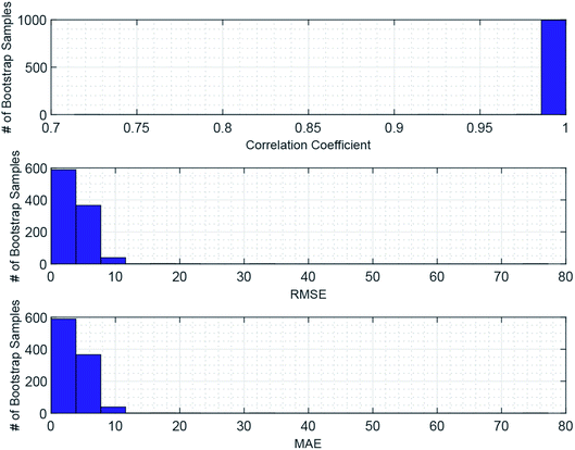
Given the small sample size (see Table 1) used, the prediction stability of the GPR is assessed through bootstrap analysis in Fig. 3, which shows that the modeling approach maintains high CCs, low RMSEs, and low MAEs over the bootstrap samples. This result suggests that the GPR might be generalized for magnetic cooling power modeling of manganite materials based on larger samples.
 |
| | Fig. 3 Bootstrap analysis of GPR prediction stability. 1000 bootstrap samples are drawn with replacements from the whole sample. Each bootstrap sample is used to train the GPR based on the Matern 5/2 kernel and constant basis function with lattice parameters standardized, and obtain the associate model performance. The histograms show distributions of the CC, RMSE, and MAE over the 1000 bootstrap samples, whose averages are 99.87%, 2.7915, and 0.9800, respectively. | |
4.3 Prediction sensitivity
Table 2 shows that GPR predictions are not so sensitive to choices of kernels or basis functions. Because predictions based on different kernel–basis function pairs are so close and nearly visually indistinguishable, they are not plotted for comparisons. However, it is worth noting that estimated model parameters are different across these kernel–basis function pairs.
Table 2 GPR prediction sensitivities to kernel and basis function choicesa
| Kernel |
Basis function |
CC |
RMSE |
RMSE/sample mean |
MAE |
MAE/sample mean |
| The final GPR model is based on the Matern 5/2 kernel and constant basis function. |
| Matern 5/2 |
Constant |
99.87% |
5.0339 |
2.10% |
1.0923 |
0.46% |
| Rational quadratic |
Constant |
99.87% |
5.0458 |
2.11% |
1.3362 |
0.56% |
| Squared exponential |
Constant |
99.87% |
5.0345 |
2.10% |
1.1389 |
0.48% |
| Exponential |
Constant |
99.87% |
5.1248 |
2.14% |
1.7993 |
0.75% |
| Matern52 |
Linear |
99.87% |
5.0339 |
2.10% |
1.0947 |
0.46% |
| Matern52 |
Pure quadratic |
99.87% |
5.0339 |
2.10% |
1.0940 |
0.46% |
5 Conclusions
The Gaussian process regression (GPR) model is developed to predict relative cooling power of manganite materials based on lattice parameters. The high correlation coefficient between the predicted and experimental magnetic cooling power, the low prediction root mean square error and mean absolute error, and stable model performance suggest the usefulness of the GPR for modeling and understanding the relationship between lattice parameters and relative cooling power. This modeling approach is straightforward and simple and requires less parameters as compared to thermodynamics models and first-principle models. It can be used as part of computational intelligence approaches for new magnetocaloric materials searches.
Conflicts of interest
There are no conflicts to declare.
References
- K. Abdouli, W. Cherif, H. Omrani, M. Mansouri, M. A. Valent, M. P. F. Graça and L. Ktari, Structural, magnetic and magneto caloric properties of La0.5Sm0.2Sr0.3Mn1−xFexO3 compounds with (0 ≤ x ≤ 0.15), J. Magn. Magn. Mater., 2019, 475, 635–642 CrossRef CAS.
- V. Basso, G. Bertotti, M. LoBue and C. P. Sasso, Theoretical approach to the magnetocaloric effect with hysteresis, J. Magn. Magn. Mater., 2005, 290, 654–657 CrossRef.
- H. Ben Khlifa, Y. Regaieg, W. Cheikhrouhou-Koubaa, M. Koubaa and A. Cheikhrouhou, Structural, magnetic and magnetocaloric properties of K-doped Pr0.8Na0.2−xKxMnO3 manganites, J. Alloys Compd., 2015, 650, 676–683 CrossRef CAS.
- A. Bettaibi, R. M'nassri, A. Selmi, H. Rahmouni, N. Chniba-Boudjada, A. Cheikhrouhou and K. Khirouni, Effect of chromium concentration on the structural, magnetic and electrical properties of praseodymium-calcium manganite, J. Alloys Compd., 2015, 650, 268–276 CrossRef CAS.
- V. Franco, J. S. Blázquez and A. Conde, Field dependence of the magnetocaloric effect in materials with a second order phase transition: a master curve for the magnetic entropy change, Appl. Phys. Lett., 2006, 89(22), 222512 CrossRef.
- V. Franco, J. S. Blázquez, J. J. Ipus, J. Y. Law, L. M. Moreno-Ramírez and A. Conde, Magnetocaloric effect: from materials research to refrigeration devices, Prog. Mater. Sci., 2018, 93, 112–232 CrossRef.
- V. Franco, T. Gottschall, K. P. Skokov and O. Gutfleisch, First-order reversal curve (FORC) analysis of magnetocaloric heusler-type alloys, IEEE Magn. Lett., 2016, 7, 1–4 Search PubMed.
- R. Gimaev, Y. Spichkin, B. Kovalev, K. Kamilov, V. Zverev and A. Tishin, Review on magnetic refrigeration devices based on HTSC materials, Int. J. Refrig., 2019, 100, 1–12 CrossRef CAS.
- K. A. GschneidnerJr, V. K. Pecharsky and A. O. Tsokol, Recent developments in magnetocaloric materials, Rep. Prog. Phys., 2005, 68(6), 1479 CrossRef.
- O. Gutfleisch, M. A. Willard, E. Brück, C. H. Chen, S. G. Sankar and J. P. Liu, Magnetic materials and devices for the 21st century: stronger, lighter, and more energy efficient, Adv. Mater., 2011, 23(7), 821–842 CrossRef CAS PubMed.
- S. Hcini, M. Boudard, S. Zemni and M. Oumezzine, Effect of Fe-doping on structural, magnetic and magnetocaloric properties of Nd0.67Ba0.33Mn1−xFexO3 manganites, Ceram. Int., 2014, 40(10), 16041–16050 CrossRef CAS.
- A. Jerbi, A. Krichene, N. Chniba-Boudjada and W. Boujelben, Magnetic and magnetocaloric study of manganite compounds Pr0.5A0.05Sr0.45MnO3 (A= Na and K) and composite, Phys. B, 2015, 477, 75–82 CrossRef CAS.
- M. Khlifi, M. Bejar, O. E. Sadek, E. Dhahri, M. A. Ahmed and E. K. Hlil, Structural, magnetic and magnetocaloric properties of the lanthanum deficient in La0.8Ca0.2−x□xMnO3 (x = 0–0.20) manganites oxides, J. Alloys Compd., 2011, 509(27), 7410–7415 CrossRef CAS.
- S. Mahjoub, M. Baazaoui, R. M'nassri, H. Rahmouni, N. C. Boudjada and M. Oumezzine, Effect of iron substitution on the structural, magnetic and magnetocaloric properties of Pr0.6Car0.1Srr0.3Mnr1−xFexOr3 (0 ≤ x ≤ 0.075) manganites, J. Alloys Compd., 2014, 608, 191–196 CrossRef CAS.
- M. Mihalik, J. Vejpravová, J. Rusz, M. Diviš, P. Svoboda, V. Sechovský and M. Mihalik, Anisotropic magnetic properties and specific-heat study of a TbFe2Si2 single crystal, Phys. Rev. B: Condens. Matter Mater. Phys., 2004, 70(13), 134405 CrossRef.
- A. Mleiki, S. Othmani, W. Cheikhrouhou-Koubaa, M. Koubaa, A. Cheikhrouhou and E. K. Hlil, Effect of praseodymium doping on the structural, magnetic and magnetocaloric properties of Sm0.55−xPrxSr0.45MnO3 (0.1 ≤ x ≤ 0.4) manganites, J. Alloys Compd., 2015, 645, 559–565 CrossRef CAS.
- P. Nisha, S. S. Pillai, M. R. Varma and K. G. Suresh, Critical behavior and magnetocaloric effect in La0.67Ca0.33Mn1−xCrxO3 (x = 0.1, 0.25), Solid State Sci., 2012, 14(1), 40–47 CrossRef CAS.
- E. Oumezzine, S. Hcini, E. K. Hlil, E. Dhahri and M. Oumezzine, Effect of Ni-doping on structural, magnetic and magnetocaloric properties of La0.6Pr0.1Ba0.3Mn1−xNixO3 nanocrystalline manganites synthesized by Pechini sol–gel method, J. Alloys Compd., 2014, 615, 553–560 CrossRef CAS.
- T. O. Owolabi, L. E. Oloore, K. O. Akande and S. O. Olatunji, Modeling of magnetic cooling power of manganite-based materials using computational intelligence approach, Neural Comput. Appl., 2019, 31(2), 1291–1298 CrossRef.
- M. H. Phan and S. C. Yu, Review of the magnetocaloric effect in manganite materials, J. Magn. Magn. Mater., 2007, 308(2), 325–340 CrossRef CAS.
- K. G. Sandeman, Magnetocaloric materials: the search for new systems, Scr. Mater., 2012, 67(6), 566–571 CrossRef CAS.
- J. Schwartz, C. C. Koch, Y. Zhang and X. Liu, Formation of bismuth strontium calcium copper oxide superconductors, US Pat., US9773962B2, September 26, 2017, https://patents.google.com/patent/US9773962B2/en.
- A. Selmi, R. M'nassri, W. Cheikhrouhou-Koubaa, N. C. Boudjada and A. Cheikhrouhou, Influence of transition metal doping (Fe, Co, Ni and Cr) on magnetic and magnetocaloric properties of Pr0.7Ca0.3MnO3 manganites, Ceram. Int., 2015, 41(8), 10177–10184 CrossRef CAS.
- A. Selmi, R. M'nassri, W. Cheikhrouhou-Koubaa, N. C. Boudjada and A. Cheikhrouhou, Effects of partial Mn-substitution on magnetic and magnetocaloric properties in Pr0.7Ca0.3Mn0.95X0.05O3 (Cr, Ni, Co and Fe) manganites, J. Alloys Compd., 2015, 619, 627–633 CrossRef CAS.
- A. Selmi, R. M'nassri, W. Cheikhrouhou-Koubaa, N. C. Boudjada and A. Cheikhrouhou, The effect of Co doping on the magnetic and magnetocaloric properties of Pr0.7Ca0.3Mn1−xCoxO3 manganites, Ceram. Int., 2015, 41(6), 7723–7728 CrossRef CAS.
- R. Thiyagarajan, S. Esakki Muthu, R. Mahendiran and S. Arumugam, Effect of hydrostatic pressure on magnetic and magnetocaloric properties of Mn-site doped perovskite manganites Pr0.6Ca0.4Mn0.96B0.04O3 (B = Co and Cr), J. Appl. Phys., 2014, 115(4), 043905 CrossRef.
- J. Töpfer and J. B. Goodenough, LaMnO3+δRevisited, J. Solid State Chem., 1997, 130(1), 117–128 CrossRef.
- Y. Zhang, S. Johnson, G. Naderi, M. Chaubal, A. Hunt and J. Schwartz, High critical current density Bi2Sr2CaCu2Ox/Ag wire containing oxide precursor synthesized from nano-oxides, Supercond. Sci. Technol., 2016, 29(9), 095012 CrossRef.
- Y. Zhang, C. C. Koch and J. Schwartz, Formation of Bi2Sr2CaCu2Ox/Ag multifilamentary metallic precursor powder-in-tube wires, Supercond. Sci. Technol., 2016, 29(12), 125005 CrossRef.
- Y. Zhang, C. C. Koch and J. Schwartz, Synthesis of Bi2Sr2CaCu2Ox superconductors via direct oxidation of metallic precursors, Supercond. Sci. Technol., 2014, 27(5), 055016 CrossRef.
- Y. Zhang and X. Xu, Fe-based superconducting transition temperature modeling through Gaussian process regression, submitted for publication.
- Y. Zhang and X. Xu, Yttrium barium copper oxide superconducting transition temperature modeling through Gaussian process regression, Comput. Mater. Sci., 2020, 179, 109583 CrossRef CAS.
- Y. Zhang and X. Xu, Disordered MgB2 superconductor critical temperature modeling through regression trees, submitted for publication.
- Y. Zhang and X. Xu, Predicting doped MgB2 superconductor critical temperature from lattice parameters using Gaussian process regression, Phys. C, 2020, 573, 1353633 CrossRef CAS.
- Y. Zhang and X. Xu, Curie temperature modeling of magnetocaloric lanthanum manganites using Gaussian process regression, J. Magn. Magn. Mater., 2020, 166998 CrossRef.
- Y. Zhang and X. Xu, Gaussian process modeling of magnetocaloric lanthanum manganites Curie temperature, submitted for publication.
- Y. Zhang and X. Xu, Machine learning the magnetocaloric effect in manganites from lattice parameters, Appl. Phys. A: Mater. Sci. Process., 2020, 126, 341 CrossRef CAS.
- Y. Zhang and X. Xu, Machine learning the magnetocaloric effect in manganites from compositions and structural parameters, AIP Adv., 2020, 10(3), 035220 CrossRef.
- Y. Zhang and X. Xu, Predicting the thermal conductivity enhancement of nanofluids using computational intelligence, Phys. Lett. A, 2020, 384, 126500 CrossRef CAS.
- Y. Zhang and X. Xu, Transformation temperature predictions through computational intelligence for NiTi-based shape memory alloys, submitted for publication.
- Y. Zhang and X. Xu, Machine learning modeling of lattice constants for half-Heusler alloys, AIP Adv., 2020, 10, 045121 CrossRef.
- Y. Zhang and X. Xu, Machine learning modeling of metal surface energy, submitted for publication.
- Y. Zhang and X. Xu, Machine learning optical band gaps of doped-ZnO films, Optik, 2020, 164808 CrossRef CAS , in press.
- Y. Zhang and X. Xu, Machine learning band gaps of doped-TiO2 photocatalysts from structural and morphological parameters, ACS Omega, 2020 Search PubMed.
Footnote |
| † The comparison is not 100% one-to-one because nine additional observations are used in ref. 19. The data are split into the training and validation sub-samples in ref. 19, where the former has 43 observations and the latter 10. We compare model performance of the GPR with that of the SVM regression19 by focusing on their 43 training observations. |
|
| This journal is © The Royal Society of Chemistry 2020 |
Click here to see how this site uses Cookies. View our privacy policy here.  Open Access Article
 * and
Xiaojie Xu
 and
and  , from an unknown distribution. A trained GPR predicts values of the response variable ynew given an input matrix xnew.
 . k(x,x′) is often parameterized by the hyperparameter, θ, and thus might be written as k(x,x′|θ). In general, different algorithms estimate β, σ2, and θ for model training and would allow specifications of b and k, as well as initial values for parameters.
 , and α is a positive-valued scale-mixture parameter. Note that σl and σf should be positive. This could be enforced through θ such that θ1 = log
![[thin space (1/6-em)]](https://www.rsc.org/images/entities/char_2009.gif) σl and θ2 = log
σl and θ2 = log![[thin space (1/6-em)]](https://www.rsc.org/images/entities/char_2009.gif) σf.
σf.


 .
. and
and  are their averages.


![[small beta, Greek, circumflex]](https://www.rsc.org/images/entities/i_char_e114.gif) of 233.9604,
of 233.9604, ![[small sigma, Greek, circumflex]](https://www.rsc.org/images/entities/i_char_e111.gif) of 0.9866,
of 0.9866, ![[small sigma, Greek, circumflex]](https://www.rsc.org/images/entities/i_char_e111.gif) l of 0.0053, and
l of 0.0053, and ![[small sigma, Greek, circumflex]](https://www.rsc.org/images/entities/i_char_e111.gif) f of 89.8778. Detailed numerical predictions are listed in Table 1 (Column 6). “□” in sample names stands for “vacancy”.
f of 89.8778. Detailed numerical predictions are listed in Table 1 (Column 6). “□” in sample names stands for “vacancy”.
