An efficient variable selection method based on random frog for the multivariate calibration of NIR spectra

Abstract

Variable selection is a critical step for spectrum modeling. In this study, a new method of variable interval selection based on random frog (RF), known as Interval Selection based on Random Frog (ISRF), is developed. In the ISRF algorithm, RF is used to search the most likely informative variables and then, a local search is applied to expand the interval width of the informative variables. Through multiple runs and visualization of the results, the best informative interval variables are obtained. This method was tested on three near infrared (NIR) datasets. Four variable selection methods, namely, genetic algorithm PLS (GA-PLS), random frog, interval random frog (iRF) and interval variable iterative space shrinkage approach (iVISSA) were used for comparison. The results show that the proposed method is very efficient to find the best interval variables and improve the model's prediction performance and interpretation.

---

Introduction

In recent years, near-infrared (NIR) spectroscopy¹ has been widely used due to its simplicity, rapidity and non-destruction of samples, and it has proven to be useful for the rapid determination of the compositions or properties of analytical samples in the fields of agriculture,² food,³ environment,⁴ etc. The main purpose of NIR spectral analysis is to construct a calibration model between the spectral variables (wavelength) and properties of the samples. However, as advances in modern spectroscopic analytical instrumentation have brought a closer observation on the samples to be analysed with high resolution, large amounts of data have poured from the analytical systems. This has also brought great challenges to the analysis of the relationship between the spectral wavelengths and the properties of analytical samples. This is the so-called “large p, small n” problem.^5,6 To address this problem, latent variable (LV) methods have been proposed, including principal component regression (PCR)⁷ and partial least squares (PLS).⁸ Although latent variables extracted from full-spectrum data reduce the impact of multi-collinearity, they are hardly interpretable. In fact, spectral data contain large amounts of redundant information and noise information. Many researchers have shown that removing irrelevant and interfering variables can significantly improve the performance of the models and enhance the interpretability of the models by selecting informative variables.^9–12 Therefore, variable selection methods have played a significant role in the analysis of high-dimensional datasets.

To date, a number of procedures have been developed for wavelength selection in the field of multivariate calibration. These procedures can be distinguished from each other either based on single wavelength selection or wavelength interval selection. Typical single wavelength selection methods include forward selection,¹³ backward elimination,¹⁴ stepwise selection,¹⁵ uninformative variable elimination (UVE),¹⁶ Monte Carlo-based UVE (MC-UVE),¹⁷ successive projection algorithm (SPA),¹⁸ iterative predictor weighting (IPW),¹⁹ competitive adaptive reweighted sampling (CARS),^20,21 random frog (RF),²² recursive weighted partial least squares (rPLS),²³ iteratively retaining informative variables (IRIV),²⁴ variable combination population analysis (VCPA),²⁵ variable iterative space shrinkage approach (VISSA),²⁶ bootstrapping soft shrinkage (BOSS),²⁷ latent projective graph (LPG),²⁸ methods based on optimization algorithms, such as genetic algorithm (GA),^29,30 particle swarm optimization (PSO),³¹ and ant colony optimization (ACO),³² and methods based on regularization, such as least absolute shrinkage and selection operator (LASSO),³³ elastic net (EN)³⁴ and sampling error profile analysis-LASSO (SEPA-LASSO).³⁵ Due to the fact that the absorption band of a functional group corresponds to a relatively short wavelength band in the spectrum, it makes more sense to find the most useful spectral band interval instead of a single spectral point and it is also easier to obtain a stable model and explain the model.³⁶ Therefore, a series of methods of wavelength interval selection have been designed, including interval PLS (iPLS),³⁷ backward iPLS (biPLS),³⁸ synergy interval PLS (siPLS),³⁹ moving window PLS (MWPLS),⁴⁰ interval partial least square with genetic algorithm (iPLS-GA),⁴¹ interval successive projection algorithm (iSPA),⁴² interval random frog (iRF),⁴³ interval variable iterative space shrinkage approach (iVISSA)⁴⁴ and ordered homogeneity pursuit LASSO (OHPL).⁴⁵ It is worth noting that most of methods mentioned above are based on model population analysis (MPA),⁴⁶ such as MC-UVE,¹⁷ CARS,^20,21 RF,^22,43 IRIV,²⁴ VCPA,²⁵ VISSA^26,44 and BOSS.²⁷ MPA is a general framework for developing new procedures in chemometrics and bioinformatics. It mainly computes the statistical information of every variable from a large population of sub-models built with a large population of variable subsets which are generated by different sampling methods. Many papers^{20,22,24–27,43,44} based on MPA have shown that there is a great improvement in model prediction ability.

If one variable is useful for modelling, other variables surrounding that variable may also be useful for modelling.⁴⁰ If different variables in an NIR spectrum have the same information, then it seems sufficient to use only one when modelling. However, there may be a phenomenon in which, although the same variable selection algorithm is used, different models are occasionally obtained. This is disadvantageous in terms of model interpretation and model stability because the results cannot be reproduced. Therefore, it is best to build the model with as many information variables as possible to obtain more stable results. In addition, the use of interval variables is more conducive to the stability of the instrument for rapid on-line measurements. Therefore, in this study, a new method called Interval Selection based on Random Frog (ISRF) is proposed to select the optimal intervals for modelling and interpretation. It is based on the RF algorithm²² and combines the selection of wavelength intervals and local searches to automatically optimize the wavelength intervals and their widths. In the ISRF algorithm, RF is used to search the most likely informative wavelengths, and then a local search is applied to expand the width of the informative wavelengths. The performance of ISRF was tested on three groups of NIR spectral datasets and compared with PLS, GA-PLS,³⁰ RF,²² iRF,⁴³ and iVISSA.⁴⁴ The results show that ISRF is an efficient wavelength interval selection method for multivariate calibration.

Theory and algorithm

Random frog coupled with PLS

Random frog is a novel selection algorithm developed for selecting cancer-related genes²² and extracting the framework of Reversible Jump Markov Chain Monte Carlo (RJMCMC).⁴⁷ However, it is noteworthy that no demanding mathematical formulation is needed and no prior distributions are required to be specified as in RJMCMC methods, which makes it easier to implement. It uses partial least squares to construct the regression model and works iteratively. Let X(n × p) define the data matrix with the spectroscopic data, while y(n × 1) defines the vector of the property of samples. X contains n samples and p variables. When modelling, both X and y were mean-centered.

RF works in four steps as follows.

Step 1. A variable subset V₀ containing Q variables is initialized randomly. V contains all p variables. Q is the number of variables (1 ≤ Q ≤ p) contained in the initialised variable set.

Step 2. Q* is generated according to a normal distribution Norm(Q,θQ). Here Q and θQ are the mean and standard deviation of this distribution, respectively. θ is a factor tuning the variance of a normal distribution. A candidate variable subset V*, which contains Q* variables, is produced as follows: (1) if Q* = Q, let V* = V₀; (2) if Q* < Q, a PLS model is first created using V₀, the absolute regression coefficient of every variable in this model is sorted and the first Q* variables with the largest absolute regression coefficients are maintained as V*; (3) if Q* > Q, first randomly select ω(Q* − Q) variables from V − V₀ as variable subset S, then build the PLS model with V₀ and S, and finally retain the Q* variables with the largest absolute regression coefficients as V*. Here, ω is a factor tuning the number of variables added to the candidate variable subset when the number of candidate variables is larger than that of current variables and its value should be larger than 1. V is the set containing all the original variables. To make this step easier to understand, an example is given as follows. Suppose V = {1, 2, 3, 4, 5, 6, 7, 8, 9, 10, 11, 12, 13, 14, 15}, V₀ = {1, 2, 3, 4, 5}, Q = 5, θ = 0.4 and ω = 2. Since Q* is generated from the normal distribution Norm(5,0.4 × 5), so V* is produced under three different situations. If Q* = 5, then V* = V₀ = {1, 2, 3, 4, 5}; if Q* < Q and assuming Q* = 4, then use V₀ to build the PLS model and retain the Q* variables with the largest absolute regression coefficients, that is V* = {2, 3, 4, 5}; if Q* > Q and assuming Q* = 7, then first compute V − V₀ = {6, 7, 8, 9, 10, 11, 12, 13, 14, 15} and choose ω(Q* − Q) variables from V − V₀, such as S = {6, 7, 8, 9}, then use V₀ ∪ S = {1, 2, 3, 4, 5, 6, 7, 8, 9} to build the PLS model and finally retain the Q* variables with the largest absolute regression coefficients, that is V* = {3, 4, 5, 6, 7, 8, 9}.

Step 3. Compute the root mean squared error of cross-validation (RMSECV) using V₀ and V* respectively, denoted as RMSECV and RMSECV*. If RMSECV* ≤ RMSECV, update V₀ as V*; else update V₀ as V* with probability ηRMSECV/RMSECV*. Then return to Step 2 until N iterations. Here, η is a parameter that is the upper bound of the probability of accepting a candidate variable subset whose performance is not better than the current variable subset. Its value is larger than 0, but less than 1.

Step 4. After N iterations, a selection probability of every variable is computed following the formula

where N denotes the number of iterations, which needs to be sufficiently large to achieve convergence. Prob_j denotes the selection probability for the jth variable and N_j denotes the times it is selected in these N models.

Here, selection probability is used as a measure of variable importance, because the more important a variable is, the more likely it is to be selected into the variable subsets for modelling.

Interval selection based on random frog (ISRF)

The ISRF algorithm proposed in this study is based on random frog coupled with PLS. Although RF is based on the analysis of a large number of sub-models sampled from the model space, there is still no guarantee that every variable selected is actually an informative variable. It is necessary to check any variable selected from RF. In addition, due to the continuity of spectral responses, the variables at nearby channels contain almost the same information. So, we expand the variable into the spectral interval, which can provide more stable results and is easier to interpret. As can be expected, the larger the selection probability of a variable is, the stronger the correlation with the properties of samples and the greater the priority of a variable to enter into the subset for building the predictive model. The detail procedure is listed here.

Step 1: descend the selection probability of each variable from RF method above. That is,

Prob₁ ≥ Prob₂ ≥ … ≥ Prob_j ≥ … ≥ Prob_p, 1 ≤ j ≤ p.

Step 2: build a series of PLS models with an increasing number of variables. In this process, if the performance of a PLS model with j variables is no better than that of the previous one with j − 1 variables, exclude the variable which was just added. This process lasts until all the variables are checked and is called filtering variables. After this step, a model M(k₁, k₂, …, k_i, …, k_q) containing q variables is obtained with selection probabilities meeting the following conditions.

Prob_k1 ≥ Prob_k2 ≥ … ≥ Prob_ki ≥ … ≥ Prob_kq

Step 3: expand the variables, which have been selected into the model M(k₁, k₂, …, k_i, …, k_q) in Step 2, to be the interval variables as follows.

(1) First initialize the model M only containing the variable k_i(i = 1).

(2) Create a new model M* by adding the adjacent variable of k_i. Compare the prediction errors of M and M* using RMSECV method, respectively denoting as RMSECV and RMSECV*. If RMSECV* < RMSECV, the adjacent variable of k_i is added into the model; in other words, update M as M* until no more adjacent variables of k_i are added.

(3) Add variable k_i+1 into model M as a new model M*.

(4) Compare the prediction errors of M and M*. If RMSECV* < RMSECV, update M as M* and go to (2), otherwise go to (3).

The model with the lowest RMSECV is obtained at last.

This strategy coupled with the RF method realizes the optimization of the locations, widths and combinations of spectral intervals.

Comparison of ISRF and iRF

iRF is also a variable interval selection method based on RF coupled with PLS. It first uses a fixed-size window that moves through the entire spectrum and obtains all the possible intervals. These overlapping intervals are treated as variable when applying RF coupled with PLS. The main characteristics of iRF are to increase both the probability that adjacent variables jointly build the model and the ease of finding the informative variable intervals. However, the disadvantage is that the size of each interval is fixed, which inevitably brings uninformative or interfering variables into the model.

In comparison, in order to overcome the overestimation of the selection probability of each variable in RF, the model constructed by ISRF method not only contains the variables with large selection probability but also uses a small number of variables with lower selection probability. In addition, the larger the selection probability of a variable is, the greater the priority of that variable and its adjacent variables is for building the predictive model. So, the selection of variable interval is not random but through expansion of the single variable with higher priority; the width of the corresponding interval is formed automatically. Finally, the model with the best variables is obtained. In summary, the ISRF method reflects the idea of progressive refinement.

Datasets

Three publicly available NIR datasets were used in this study to validate the ISRF method.

Soy moisture dataset

This dataset consists of 54 soy flour samples. The samples are measured on an NIR spectrometer. Each spectrum was recorded at intervals of 8 nm from 1104 nm to 2496 nm (175 spectral points). The moisture value was considered the property of interest. In addition, the dataset was divided into a calibration set (40 samples) and a validation set (14 samples) in terms of the ref. 48.

Corn dataset

This is a benchmark NIR spectra dataset of corn that is freely available at http://www.eigenvector.com/data/Corn/index.html. This dataset consists of 80 samples of corn measured on three different NIR spectrometers. Each spectrum was recorded at intervals of 2 nm within the range from 1100 nm to 2498 nm (700 wavelength points). In this study, the NIR spectra measured on the m5 instrument were considered and the moisture values were used as the response. 64 samples were used as a calibration set and the other 16 samples were used as the validation set according to the Kennard–Stone (KS) method.⁴⁹

Wheat dataset

This dataset³⁰ consists of 100 wheat samples and each spectrum was compressed into 175 variables from 701 spectral variables in the range 1100–2500 nm at an interval of 2 nm.⁵⁰ The protein content of wheat samples was used as the response. 80 samples of the dataset were used for the calibration set and 20 samples were used for the validation set by the Kennard–Stone (KS) method.⁴⁹

Results and discussion

To evaluate the performance of ISRF, five promising wavelength selection methods, PLS, GA-PLS, RF, iRF, and iVISSA, were considered for comparison. All the data were mean-centred before modelling. The root mean square error of cross-validation (RMSECV), root mean square error of the calibration set (RMSEC) and root mean square error of the validation set (RMSEP) were used to assess model performance. In addition, the number of variables selected (nVAR) and the number of optimal latent variables (nLV) were also recorded. Except for PLS, the results of other methods cannot be reproduced due to random sampling. To reduce this randomness, each method was conducted 50 times for evaluation of reproducibility and stability.

As discussed before, there are five parameters, N, Q, θ, ω, and η, which should be initialized before running the RF method. The larger N is, the more likely and stable the RF method is to get the best variable set but the higher the running time is. As for the parameters θ, ω, and η, they do not have significant influences on the results according to the work of ref. 22. For the parameter Q, different values were tested on three datasets, such as 2, 10, 30, and 50. As can be seen from Table 1, when the number of iterations is 10 000, the value of Q does not have significant effect on the model results, which is consistent with the ref. 22. In this study, the parameters N, Q, θ, ω and η were set to 10 000, 50, 0.3, 3 and 0.1, respectively.

Table 1 Results of the RMSECV of the PLS model constructed by RF algorithm with 5-fold cross-validation and statistical results with the form mean value ± standard deviation in 20 runs

Q	Soy moisture	Corn	Wheat
2	0.7296 ± 0.0018	0.00028 ± 0.00001	0.3073 ± 0.0044
10	0.7295 ± 0.0011	0.00028 ± 0.00001	0.3075 ± 0.0022
30	0.7297 ± 0.0009	0.00028 ± 0.00001	0.3077 ± 0.0040
50	0.7298 ± 0.0014	0.00028 ± 0.00001	0.3074 ± 0.0033

---

Soy moisture dataset

For this dataset, the maximum number of latent variables was set at 4 by 5-fold cross-validation on the full spectra, according to the ref. 44. The results of variable selection methods PLS, GA-PLS, RF, iRF and iVISSA are displayed in Table 2. As can be seen, compared with the full spectrum, all of the selection methods showed improved performance. In this experiment, iRF showed the lowest RMSEP (0.9643), followed by RF (0.9834), GA-PLS (0.9843), ISRF (1.0151) and iVISSA (1.0354), while GA-PLS showed the lowest RMSEP (0.9873), followed by iVISSA (0.9950) and iRF (0.9967) in the ref. 44. In fact, because these variable selection algorithms use random methods, the results are not unique; the order of the performances of models using these variable selection algorithms will change when the algorithms are re-executed, but they are all within the allowable error range. As can be seen from Table 2, the differences of the average RMSECV, RMSEC and RMSEP values of these variable selection methods are not obvious. So, a Wilcoxon signed rank test is applied to compare RMSEP values with median values. The results showed there was significant difference between ISRF and other methods at the 5% significance level. ISRF was slightly worse than iRF, RF and GA-PLS, but was better than iVISSA.

Table 2 Results of soy dataset. nVAR: the number of variables; nLV: the number of latent variables; RMSEC: the root-mean-square error of calibration; RMSECV: the root-mean-square error of cross-validation; RMSEP: the root-mean-square error of prediction; statistical results with the form mean value ± standard deviation in 50 runs

Method	nVAR	nLV	RMSECV	RMSEC	RMSEP
PLS	175	4	0.8702	0.7230	1.1090
GA-PLS	16.04 ± 5.3755	2.12 ± 0.4798	0.7289 ± 0.0054	0.7116 ± 0.0162	0.9843 ± 0.0233
RF	18.78 ± 10.2684	2.00 ± 0.0000	0.7298 ± 0.0013	0.7070 ± 0.0012	0.9834 ± 0.0087
iRF	23.12 ± 2.9182	2.36 ± 0.4849	0.7403 ± 0.0047	0.7118 ± 0.0038	0.9643 ± 0.0078
iVISSA	25.40 ± 0.9258	2.00 ± 0.0000	0.7273 ± 0.0014	0.7031 ± 0.0004	1.0354 ± 0.0012
ISRF	6.12 ± 5.5200	2.92 ± 0.4445	0.7224 ± 0.0066	0.6934 ± 0.0073	1.0151 ± 0.0360

---

It is worth noting that the number of variables selected by different algorithms varies widely. ISRF showed the least variables (6.12), followed by GA-PLS (16.04), RF (18.78), iRF (23.12) and iVISSA (25.4). The RMSECV of the union of the first top n variables ranked by averaging the RF methods 50 times was computed and is displayed in Fig. 1. As can be seen, the model with the top 31 variables has the lowest RMSECV (0.7292) on the calibration set, but they are not the best variable combination. The RMSECV value of the model built using the three variables, one of which is not in the first top 31 variables, marked in red on Fig. 1, can reach 0.7303. In Fig. 1, as the number of variables increases, RMSECV does not decrease continuously, which indicates that some variables that make RMSECV rise suddenly may be uninformative variables or interference variables. These variables may be not good for subsequent variable interval expansion and need to be eliminated. So, there are fewer variables in the model built with variables by ISRF than that in those built with variables selected by RF alone with lowest RMSECV value.

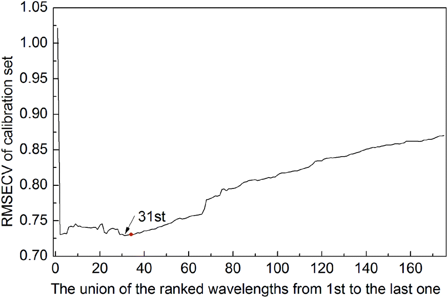Fig. 1 The RMSECV of the union of the top ranked wavelengths from 1st to last (175th) on the soy dataset. The top 31 wavelengths are the optimal wavelengths with the lowest RMSECV on the calibration set.

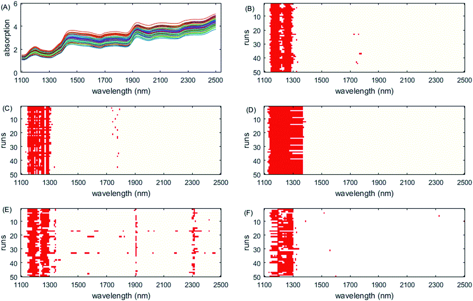
The selected variables are shown in Fig. 2. All methods except PLS select the informative region between 1944 nm and 2172 nm. They correspond to water absorption and the combination of O–H bonds.⁴⁴ Except ISRF and iRF, other algorithms have also chosen the interval 2480–2500 nm; however, there is no chemical explanation as to whether these variables are informative variables. It can be seen from Fig. 2 that in the 50 run tests, the variables selected by iVISSA are basically the same, so the iVISSA algorithm is relatively stable, but the results are not optimal. For GA-PLS, RF and iRF, the variables selected are basically irregular. For ISRF, we find that there is a certain complementarity between the selected intervals, although this feature is not very obvious in this dataset. Complementarity is defined here that the absence of variables in an important interval requires the addition of other interval variables to achieve a good model. This complementarity is mainly due to the selection probability of variables obtained by RF method being changed, leading to change in the order of interval expansion in each test run. It is this change that makes it easier to find the most informative variable intervals. In order to better demonstrate the complementarity between the variable intervals, we re-rank the results of the 50 tests according to the RMSEP value. In Fig. 6, the model performance decreases from top to bottom. As can be seen from Fig. 6A, in the 1st, 2nd, 3rd, 9th, and 10th tests, some important variables in the interval 2000–2024 nm are not included, so the variables in the interval 2072–2104 nm need to be supported to improve the prediction ability of the model, which indicates these two regions are two informative variable intervals. The variables contained in these two intervals are also selected as informative variables by GA-PLS, iRF and iVISSA. In the model built with these two variable intervals (9 variables), the obtained RMSEC and RMSEP were 0.6662 and 0.8831, respectively. This result is better than those obtained by other methods.

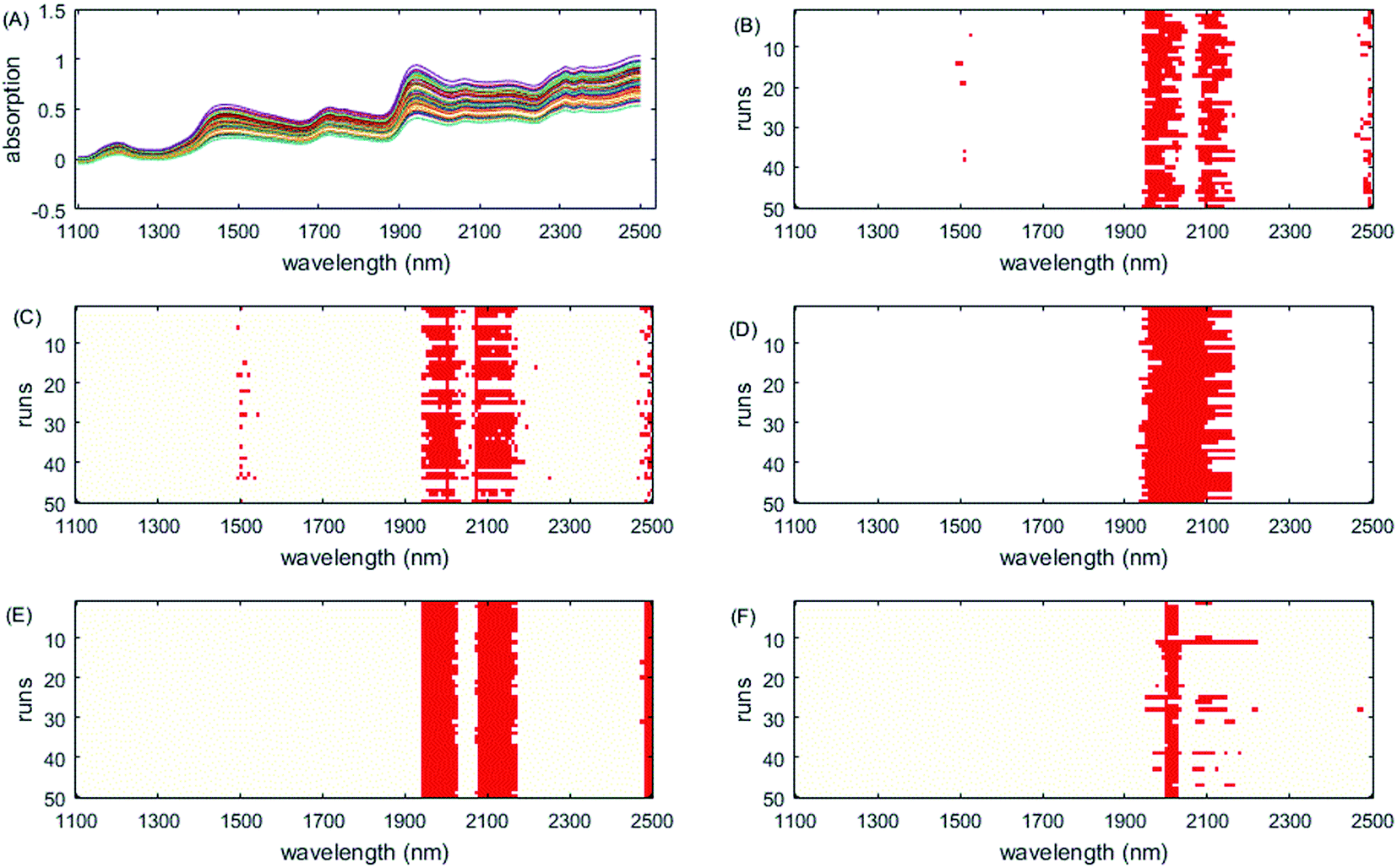Fig. 2 Wavelengths selected by different methods on the soy dataset. (A) Original spectra, (B) GA-PLS, (C) RF, (D) iRF, (E) iVISSA and (F) ISRF.

Corn dataset

In this dataset, the maximum number of latent variables was set at 10 by 5-fold cross-validation on the full spectra, according to the ref. 44. The results of the variable selection methods, PLS, GA-PLS, RF, iRF and iVISSA, are summarized in Table 3. As can be seen, compared with the full spectrum, all of the selection methods show great improvement on the test set. GA-PLS has the fewest variables but the worst result, compared with other variable selection methods. Compared with iRF and iVISSA, ISRF selects the fewest variables and shows the best prediction ability in terms of RMSECV, RMSEC and RMSEP. A Wilcoxon signed rank test is applied to compare RMSEP values with median values. The results showed there was no significant difference between ISRF and RF at the 5% significance level. There was significant difference between ISRF and GA-PLS, iRF, and iVISSA at the 5% significance level.

Table 3 Results of corn dataset. nVAR: the number of variables; nLV: the number of latent variables; RMSEC: the root-mean-square error of calibration; RMSECV: the root-mean-square error of cross-validation; RMSEP: the root-mean-square error of prediction; statistical results with the form mean value ± standard deviation in 50 runs

Method	nVAR	nLV	RMSECV	RMSEC	RMSEP
PLS	700	10	0.0187	0.0142	0.0192
GA-PLS	5.36 ± 1.2249	5.86 ± 1.4709	0.00031 ± 0.00001	0.01180 ± 0.05240	0.01010 ± 0.04240
RF	6.84 ± 2.8526	6.70 ± 2.7049	0.00028 ± 0.00001	0.00025 ± 0.00002	0.00037 ± 0.00003
iRF	42.36 ± 3.0600	10.00 ± 0.0000	0.00250 ± 0.00012	0.00120 ± 0.00021	0.00210 ± 0.00036
iVISSA	16.60 ± 3.8386	9.86 ± 0.4953	0.00040 ± 0.00017	0.00027 ± 0.00008	0.00038 ± 0.00014
ISRF	9.68 ± 1.9213	9.04 ± 1.3845	0.00030 ± 0.00000	0.00026 ± 0.00000	0.00037 ± 0.00002

---

The selected variables on the corn dataset are displayed in Fig. 3. All the variable selection methods select the two informative regions around 1900 nm and 2100 nm, which correspond to water absorption⁵¹ and the combination of O–H bonds,⁴⁰ respectively. Although RF chooses some variables from these two interval variables each time, it also chooses other variables scattered in different locations, which is not easy for interpretation of the properties of samples. In addition, the interval widths of GA-PLS are too narrow, failing to include more informative interval variables, while the interval widths of iRF are too large, including more uninformative variables, both leading to relatively high prediction error. iVISSA uses more variables to achieve comparable results to ISRF. In this corn dataset, the complementarity between the selected intervals is very obvious and missing one of these two regions does not build a satisfactory model (Fig. 6B). Through visualization of the results, the intervals 1896–1912 nm and 2106–2114 nm are found to be two informative variable intervals. Among these variables, 1898–1912 nm and 2106–2114 nm are also selected as informative variables by iRF, iVISSA and GA-PLS and 1896 nm is selected as informative by iRF and iVISSA. In the model built with these two variable intervals (14 variables), the obtained RMSEC and RMSEP were 0.00025 and 0.00038, respectively.

Fig. 3 Wavelengths selected by different methods on the corn dataset. (A) Original spectra, (B) GA-PLS, (C) RF, (D) iRF, (E) iVISSA and (F) ISRF.

It is noteworthy that the informative variable intervals obtained in the soy dataset above are different from those of this corn dataset. One of intervals for the soy dataset is around 2000 nm, while it is around 1900 nm for the corn dataset. Another interval is very close, around 2100 nm for the two datasets. This reveals that informative variable intervals can be different for the same property of different samples.

Wheat dataset

The results of the wheat protein dataset are shown in Table 4. In this experiment, variable selection methods, except GA-PLS, can achieve better results with a smaller number of variables than the full spectrum. Among them, the ISRF method selects the fewest informative variables. A Wilcoxon signed rank test is applied to compare RMSEP values with median values. The results showed there was no significant difference between ISRF and RF at the 5% significance level. However, there was significant difference between ISRF and GA-PLS, iRF, and iVISSA at the 5% significance level.

Table 4 Results of the wheat dataset. nVAR: the number of variables; nLV: the number of latent variables; RMSEC: the root-mean-square error of calibration; RMSECV: the root-mean-square error of cross-validation; RMSEP: the root-mean-square error of prediction; statistical results with the form mean value ± standard deviation in 50 runs

Method	nVAR	nLV	RMSECV	RMSEC	RMSEP
PLS	175	10	0.6007	0.4038	0.2585
GA-PLS	17.78 ± 2.8805	9.16 ± 2.4525	0.3079 ± 0.0049	0.2667 ± 0.0233	0.2658 ± 0.0369
RF	16.82 ± 3.7071	8.16 ± 1.4049	0.3074 ± 0.0029	0.2652 ± 0.0159	0.2195 ± 0.0286
iRF	28.06 ± 4.5284	8.58 ± 0.9278	0.2969 ± 0.0098	0.2551 ± 0.0076	0.2472 ± 0.0089
iVISSA	19.20 ± 7.1514	8.80 ± 1.0498	0.3136 ± 0.0165	0.2648 ± 0.0164	0.2182 ± 0.0385
ISRF	14.42 ± 1.8526	8.12 ± 0.9179	0.3046 ± 0.0131	0.2639 ± 0.0108	0.2176 ± 0.0426

---

Due to the ISRF method being based on the RF method, Fig. 4 displays the RMSECV of the union of the first top n variables ranked by averaging the RF method 50 times. As can be seen, the model with the top 22 variables has the lowest RMSECV (0.3042) on the calibration set, but they are not the best variable combination. The RMSECV of the union of the 13th to 22nd of the ranked variables does not decrease continuously, which implies that these variables may be uninformative variables or interference variables. After running Step 1 of the ISRF method, equivalent results can be achieved with only 13 variables, two of which are not among the first 22 variables, as marked on Fig. 4 with red circles.

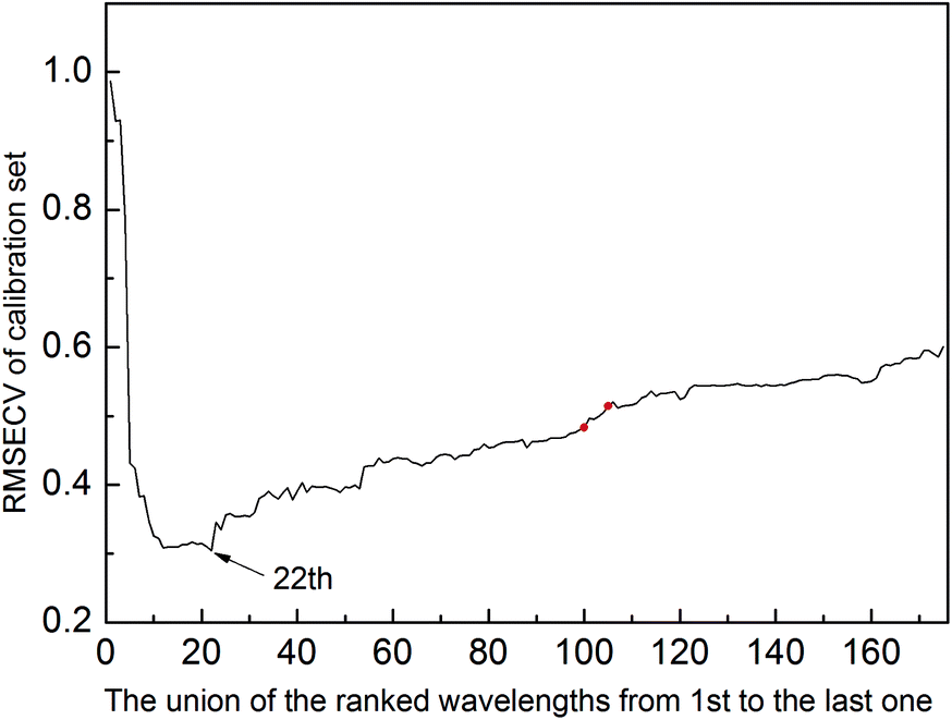Fig. 4 The RMSECV of the union of the top ranked wavelengths from 1st to last (175th) on the wheat dataset. The top 22 wavelengths are the optimal wavelengths with the lowest RMSECV on the calibration set.

The selected variables on this dataset are displayed in Fig. 5. All methods select the informative region around 1100–1300 nm, which is consistent with the results of the literature.^52,53 However, as iRF uses a fixed window size, it has a wide width of interval and iVISSA additionally selects variables from other intervals. Through the visualization of the 50 run test results, the complementarity between the selected intervals of the ISRF method is very obvious (Fig. 6C). The absence of variables in the interval 1204–1308 nm leads to the addition of the interval 1164–1204 nm, indicating that these variable intervals are the informative variables. Moreover, all these variables are also selected as informative variables by iRF, iVISSA and GA-PLS methods. In the model built with this interval (19 variables), the obtained RMSEC and RMSEP were 0.2654 and 0.1757, respectively. This result is the best compared with other methods.

Fig. 5 Wavelengths selected by different methods on the wheat dataset. (A) Original spectra, (B) GA-PLS, (C) RF, (D) iRF, (E) iVISSA and (F) ISRF.

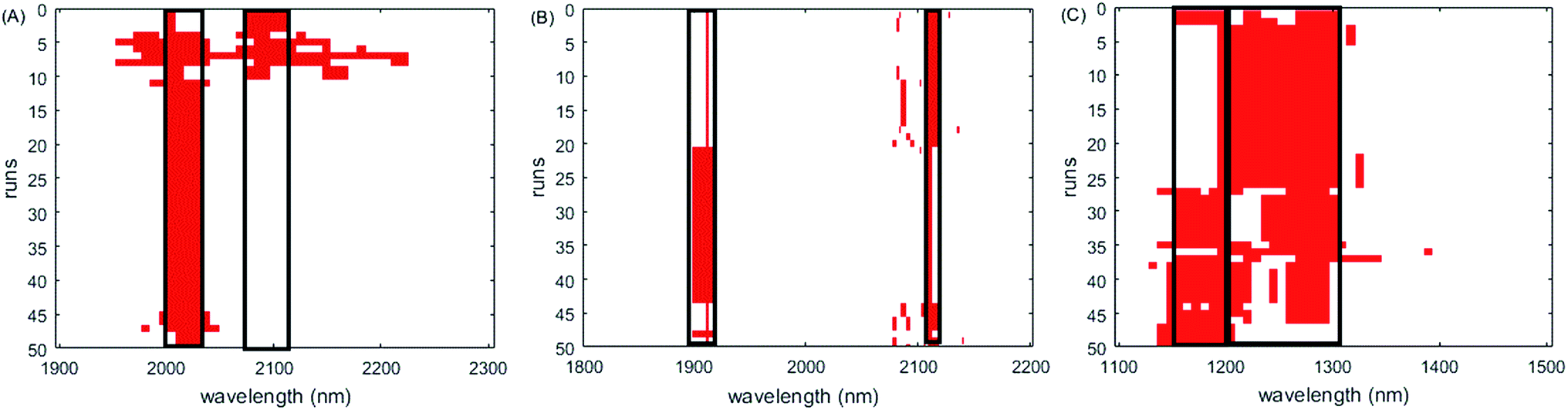Fig. 6 Wavelengths selected by ISRF on three datasets. (A) Soy dataset, (B) corn dataset, and (C) wheat dataset. The intervals marked by black blocks are the final variable composition.

Algorithm performance comparison

From the results above, we can see that, compared with other algorithms, the ISRF algorithm obtains comparable results with the fewest variables of the three data sets, which makes establishment of the prediction model easier. Each algorithm has its advantages and disadvantages and our algorithm does not seem to be optimal in terms of model stability. But it is precisely this unstable performance that helps us find useful informative variables. As can be seen from Fig. 6, through 50 runs, we found that there exists a certain complementarity between the intervals of the informative variables selected. The performance decreases in the absence of any interval, which is particularly obvious in Fig. 6B and C. It is also a good choice to visualize the results when studying the features of variables selected by the variable selection algorithm because the result of each run of the algorithm may be different. Therefore, we run each algorithm 50 times and take the average running time over these 50 runs as the criterion for assessing the time efficiency of the algorithm. Taking the corn data set containing 700 variables as an example, the average running times of iVISSA, iRF, GA-PLS, RF and ISRF are 634 s, 165 s, 81 s, 76 s and 70 s, respectively. So, our algorithm has a slight advantage for time.

Conclusions

This study proposes a new method for variable selection based on the RF method, called Interval Selection based on Random Frog (ISRF). Tested on three NIR datasets, ISRF shows the capacity to automatically optimize the positions and widths of intervals and obtains variable intervals with good prediction ability. In addition, through multiple runs of ISRF method and visualization of the results, it can help to quickly find the best informative intervals, which are more reasonable and easier to interpret for the model. It can be said that ISRF is an efficient method to be applied for spectral calibration.

Conflicts of interest

There are no conflicts to declare.

Acknowledgements

This work was supported by the National Natural Science Foundation of China (Grants No. 31871571), Shanxi Provincial Key Research and Development Project, China (Grants No. 201903D211002 and Grants No. 201603D221037-3), China Postdoctoral Science Foundation (Grants No. 2017M621105), Shanxi Excellent Doctor financial Foundation (Grants No. SXYBKY2018040), Youth Science and Technology Research Fund of Shanxi Province Applied Basic Research Project (Grants No. 201701D221105) and the Science and Technology Innovation Fund of Shanxi Agricultural University (Grants No. 2015ZZ03, Grants No. 201308).

References

1. C. Pasquini, J. Braz. Chem. Soc., 2003, 14, 198–219.
2. B. Stenberg, R. A. V. Rossel, A. M. Mouazen and J. Wetterlind, in Advances in agronomy, Elsevier, 2010, vol. 107, pp. 163–215.
3. S. Sans, J. Ferré, R. Boqué, J. Sabaté, J. Casals and J. Simó, Food Chem., 2018, 262, 178–183.
4. A. Gredilla, S. F.-O. de Vallejuelo, N. Elejoste, A. de Diego and J. M. Madariaga, TrAC, Trends Anal. Chem., 2016, 76, 30–39.
5. E. Candes and T. Tao, Annals of Statistics, 2007, 35, 2313–2351.
6. I. M. Johnstone and D. M. Titterington, Statistical challenges of high-dimensional data, The Royal Society Publishing, 2009.
7. N. M. Al-Kandari and I. T. Jolliffe, Environmetrics, 2005, 16, 659–672.
8. S. Wold, M. Sjöström and L. Eriksson, Chemom. Intell. Lab. Syst., 2001, 58, 109–130.
9. T. Mehmood, K. H. Liland, L. Snipen and S. Sæbø, Chemom. Intell. Lab. Syst., 2012, 118, 62–69.
10. C. H. Spiegelman, M. J. McShane, M. J. Goetz, M. Motamedi, Q. L. Yue and G. L. Coté, Anal. Chem., 1998, 70, 35–44.
11. Q. Wang, H.-D. Li, Q.-S. Xu and Y.-Z. Liang, Analyst, 2011, 136, 1456–1463.
12. Z. Xiaobo, Z. Jiewen, M. J. Povey, M. Holmes and M. Hanpin, Anal. Chim. Acta, 2010, 667, 14–32.
13. F. G. Blanchet, P. Legendre and D. Borcard, Ecology, 2008, 89, 2623–2632.
14. J. M. Sutter and J. H. Kalivas, Microchem. J., 1993, 47, 60–66.
15. S. Derksen and H. J. Keselman, Br. J. Math. Stat. Psychol., 1992, 45, 265–282.
16. V. Centner, D.-L. Massart, O. E. de Noord, S. de Jong, B. M. Vandeginste and C. Sterna, Anal. Chem., 1996, 68, 3851–3858.
17. W. Cai, Y. Li and X. Shao, Chemom. Intell. Lab. Syst., 2008, 90, 188–194.
18. M. C. U. Araújo, T. C. B. Saldanha, R. K. H. Galvao, T. Yoneyama, H. C. Chame and V. Visani, Chemom. Intell. Lab. Syst., 2001, 57, 65–73.
19. M. Forina, C. Casolino and C. Pizarro Millan, J. Chemom., 1999, 13, 165–184.
20. H. Li, Y. Liang, Q. Xu and D. Cao, Anal. Chim. Acta, 2009, 648, 77–84.
21. K. Zheng, Q. Li, J. Wang, J. Geng, P. Cao, T. Sui, X. Wang and Y. Du, Chemom. Intell. Lab. Syst., 2012, 112, 48–54.
22. H.-D. Li, Q.-S. Xu and Y.-Z. Liang, Anal. Chim. Acta, 2012, 740, 20–26.
23. Å. Rinnan, M. Andersson, C. Ridder and S. B. Engelsen, J. Chemom., 2014, 28, 439–447.
24. Y.-H. Yun, W.-T. Wang, M.-L. Tan, Y.-Z. Liang, H.-D. Li, D.-S. Cao, H.-M. Lu and Q.-S. Xu, Anal. Chim. Acta, 2014, 807, 36–43.
25. Y.-H. Yun, W.-T. Wang, B.-C. Deng, G.-B. Lai, X.-b. Liu, D.-B. Ren, Y.-Z. Liang, W. Fan and Q.-S. Xu, Anal. Chim. Acta, 2015, 862, 14–23.
26. B.-c. Deng, Y.-h. Yun, Y.-z. Liang and L.-z. Yi, Analyst, 2014, 139, 4836–4845.
27. B.-C. Deng, Y.-H. Yun, D.-S. Cao, Y.-L. Yin, W.-T. Wang, H.-M. Lu, Q.-Y. Luo and Y.-Z. Liang, Anal. Chim. Acta, 2016, 908, 63–74.
28. X. Shao, G. Du, M. Jing and W. Cai, Chemom. Intell. Lab. Syst., 2012, 114, 44–49.
29. R. Leardi and A. L. Gonzalez, Chemom. Intell. Lab. Syst., 1998, 41, 195–207.
30. R. Leardi, J. Chemom., 2000, 14, 643–655.
31. Q. Shen, J.-H. Jiang, C.-X. Jiao, S.-Y. Huan, G.-l. Shen and R.-Q. Yu, J. Chem. Inf. Comput. Sci., 2004, 44, 2027–2031.
32. M. Shamsipur, V. Zare-Shahabadi, B. Hemmateenejad and M. Akhond, J. Chemom., 2006, 20, 146–157.
33. R. Tibshirani, Journal of the Royal Statistical Society: Series B (Methodological), 1996, 58, 267–288.
34. H. Zou and T. Hastie, Journal of the Royal Statistical Society: Series B (Statistical Methodology), 2005, 67, 301–320.
35. R. Zhang, F. Zhang, W. Chen, H. Yao, J. Ge, S. Wu, T. Wu and Y. Du, Chemom. Intell. Lab. Syst., 2018, 175, 47–54.
36. A. Höskuldsson, Chemom. Intell. Lab. Syst., 2001, 55, 23–38.
37. L. Nørgaard, A. Saudland, J. Wagner, J. P. Nielsen, L. Munck and S. B. Engelsen, Appl. Spectrosc., 2000, 54, 413–419.
38. R. Leardi and L. Nørgaard, J. Chemom., 2004, 18, 486–497.
39. Q. Chen, J. Zhao, M. Liu, J. Cai and J. Liu, J. Pharm. Biomed. Anal., 2008, 46, 568–573.
40. J.-H. Jiang, R. J. Berry, H. W. Siesler and Y. Ozaki, Anal. Chem., 2002, 74, 3555–3565.
41. Q. Chen, P. Jiang and J. Zhao, Spectrochim. Acta, Part A, 2010, 76, 50–55.
42. A. de Araújo Gomes, M. R. Alcaraz, H. C. Goicoechea and M. C. U. Araújo, Anal. Chim. Acta, 2014, 811, 13–22.
43. Y.-H. Yun, H.-D. Li, L. R. Wood, W. Fan, J.-J. Wang, D.-S. Cao, Q.-S. Xu and Y.-Z. Liang, Spectrochim. Acta, Part A, 2013, 111, 31–36.
44. B.-C. Deng, Y.-H. Yun, P. Ma, C.-C. Lin, D.-B. Ren and Y.-Z. Liang, Analyst, 2015, 140, 1876–1885.
45. Y.-W. Lin, N. Xiao, L.-L. Wang, C.-Q. Li and Q.-S. Xu, Chemom. Intell. Lab. Syst., 2017, 168, 62–71.
46. H.-D. Li, Y.-Z. Liang, D.-S. Cao and Q.-S. Xu, TrAC, Trends Anal. Chem., 2012, 38, 154–162.
47. P. J. Green, Biometrika, 1995, 82, 711–732.
48. M. Forina, G. Drava, C. Armanino, R. Boggia, S. Lanteri, R. Leardi, P. Corti, P. Conti, R. Giangiacomo and C. Galliena, Chemom. Intell. Lab. Syst., 1995, 27, 189–203.
49. R. W. Kennard and L. A. Stone, Technometrics, 1969, 11, 137–148.
50. J. H. Kalivas, Chemom. Intell. Lab. Syst., 1997, 37, 255–259.
51. D. Jouan-Rimbaud, D.-L. Massart, R. Leardi and O. E. De Noord, Anal. Chem., 1995, 67, 4295–4301.
52. W. Wang, Y.-H. Yun, B. Deng, W. Fan and Y. Liang, RSC Adv., 2015, 5, 95771–95780.
53. Y.-H. Yun, D.-S. Cao, M.-L. Tan, J. Yan, D.-B. Ren, Q.-S. Xu, L. Yu and Y.-Z. Liang, Chemom. Intell. Lab. Syst., 2014, 130, 76–83.

---