DOI:
10.1039/D0RA00669F
(Paper)
RSC Adv., 2020,
10, 19258-19275
Fast automated processing of AFM PeakForce curves to evaluate spatially resolved Young modulus and stiffness of turgescent cells†
Received
21st January 2020
, Accepted 8th May 2020
First published on 20th May 2020
Abstract
Atomic Force Microscopy (AFM) is a powerful technique for the measurement of mechanical properties of individual cells in two (x × y) or three (x × y × time) dimensions. The instrumental progress makes it currently possible to generate a large amount of data in a relatively short time, which is particularly true for AFM operating in so-called PeakForce tapping mode (Bruker corporation). The latter corresponds to an AFM probe that periodically hits the sample surface while the pico-newton level interaction force is recorded from cantilever deflection. The method provides unprecedented high-resolution (a few tens of nm) imaging of the mechanical features of soft biological samples (e.g. bacteria, yeasts) and of hard abiotic surfaces (e.g. minerals). The rapid conversion of up to several tens of thousands spatially resolved force curves typically collected in AFM PeakForce tapping mode over a given cell surface area into comprehensive nanomechanical information requires the development of robust data analysis methodologies and dedicated numerical tools. In this work, we report an automated algorithm for (i) a rapid and unambiguous detection of the indentation regimes corresponding to non-linear and linear deformations of bacterial surfaces upon compression by the AFM probe, (ii) the subsequent evaluation of the Young modulus and cell surface stiffness, and (iii) the generation of spatial mappings of relevant nanomechanical properties at the single cell level. The procedure involves consistent evaluation of the contact point between the AFM probe and sample biosurface and that of the threshold indentation value marking the transition between non-linear and linear deformation regimes. For comparison purposes, the former regime is here analyzed on the basis of Hertz and Sneddon models corrected or not for effects of finite sample thickness. Analysis of AFM measurements performed on a selected Escherichia coli strain is detailed to demonstrate the feasibility, rapidity and robustness of the here-proposed PeakForce data treatment process. The flexibility of the algorithm allows consideration of force curve parameterizations other than that detailed here, which may be desired for investigation of e.g. eukaryotes nanomechanics. The performance of the adopted Hertz-based and Sneddon-based contact mechanics formalisms in recovering experimental data and in identifying nanomechanical heterogeneities at the bacterium scale is further thoroughly discussed.
1. Introduction
Atomic Force Microscopy (AFM) is based on the analysis of a given sample surface scanned by a local probe of given geometry and chemical composition.1 This technique makes it possible to map locally the defining physical and chemical properties of various abiotic and biological materials like minerals and bacteria, e.g. electrostatic charge,2 hydrophobic/hydrophilic balance,3–5 surface elasticity,6 and surface depressions/asperities,7 under well-controlled vacuum,8 liquid,9 or ambient10 environments. The force operational between the probe and the sample surface leads to bending of the cantilever that supports the probe. The resulting change in probe deflection is measured via a dedicated optical system, and so is the vertical position of the sample surface modulated via piezoelectric scanning. In turn, to each pixel of the probed sample surface is associated a force versus separation or indentation curve, depending on whether or not sample and probe are in contact. Physical models are then required to extract the desired spatially resolved physical or chemical features of the sample from the force measurements performed over the whole scanned sample surface area. Atomic force microscopy (AFM) is now recognized as a valuable tool for measuring mechanical characteristics of biological samples like bacteria, yeasts or animal and human cells.11,12 Via the acquisition of such nanomechanical properties used as proxies to follow (bio)surface reactivity patterns, AFM provides a way to apprehend the impact of various factors such as temperature, humidity or medium salinity on e.g. biomaterial swelling features.13,14 The technique further allows the analysis of the effects of underlying substrate on cellular stiffness,15 or the investigation of drugs action on biological surface integrity,16 on cell–cell interactions,17 cell migration18,19 and on pathogenicity.20,21 The mechanical characterization of biological surfaces has gained a prominent position in a large spectrum of applications, e.g. in (micro)biology, pharmaceutics, environmental sciences and cell engineering.16,22–24
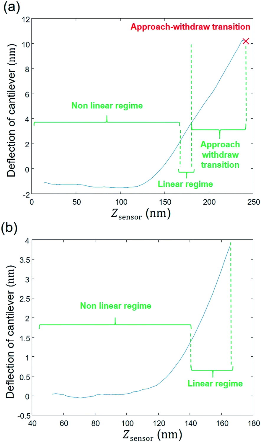
Over the last ten years, the need to lower the limits of spatial detection for addressing the biomolecular processes that control cells response to changes of neighboring environments, has given rise to the development of faster and more accurate force curve measurement technologies, in particular the PeakForce AFM tapping mode (Bruker technology).25,26 This mode of force curves acquisition allows a precise control of the sample to AFM probe interactions and a high resolution (nanometer scale) for AFM surface imaging. Methodologies differ according to e.g. sinusoidal or linear paths (the former is the one considered in this study) imposed to the probe upon approach/withdraw to/from the sample surface.27 The magnitude of the forces applied on the samples lies in the pico- to nano-newton range, which preserves probe shape and prevents samples damage during measurements, a feature that is particularly attractive when studying fragile biological structures (Fig. 1a). The amount of data typically generated during an AFM experiment may be large, which is partly due to the rapidity and relative simplicity in acquiring data by PeakForce tapping mode (e.g. 65![[thin space (1/6-em)]](https://www.rsc.org/images/entities/char_2009.gif) 536 force curves recorded on a 500 × 500 nm2 bacteria surface for a total experiment duration of ca. 4 minutes at 1 Hz scan). As a consequence, the development of efficient data treatments and of accompanying numerical tools has become mandatory for a robust exploitation and interpretation of spatially resolved force curves measurements. Fig. 1a provides a schematic representation for the measurement principle of nanomechanical interactions between an AFM probe and a soft biological sample (here a bacterium) in PeakForce tapping mode. As a first order approach, the force versus indentation curves constructed from raw data measured on bacteria may be decomposed into a non-linear and linear (or compliance) regime operational at sufficiently weak and large indentation values, respectively (Fig. 1b).23 The former regime reflects the propensity of the peripheral cell envelope to deform upon compression by the AFM probe, a feature that is quantified by the value of the Young modulus (E) or elasticity. The latter linear regime arises from the internal cell (turgor) pressure that counteracts the force exerting on the cell surface via the probe.28 The intracellular turgor (or hydrostatic) pressure is known to be operational in all bacteria and also in fungi and plants.14,23,29 For turgescent cells, the linear compliance regime is always measurable providing the magnitude of the loading force is sufficiently large depending on how rigid the cell envelope is. In practice, this turgor pressure may be expressed in terms of a so-called cell spring constant or stiffness (kcell) that can be estimated from the slope of the force versus indentation curve in the compliance regime.23,28,30 Various theories of contact mechanics are classically adopted to evaluate Young modulus from raw force measurements in the non-linear indentation regime, e.g. the Hertz,31 Johnson–Kendall–Roberts (JKR)32 or Derjaguin–Muller–Toporov (DMT)33 models whose validity differs according to AFM probe size/geometry, material stiffness or extent of AFM probe/material adhesion.
536 force curves recorded on a 500 × 500 nm2 bacteria surface for a total experiment duration of ca. 4 minutes at 1 Hz scan). As a consequence, the development of efficient data treatments and of accompanying numerical tools has become mandatory for a robust exploitation and interpretation of spatially resolved force curves measurements. Fig. 1a provides a schematic representation for the measurement principle of nanomechanical interactions between an AFM probe and a soft biological sample (here a bacterium) in PeakForce tapping mode. As a first order approach, the force versus indentation curves constructed from raw data measured on bacteria may be decomposed into a non-linear and linear (or compliance) regime operational at sufficiently weak and large indentation values, respectively (Fig. 1b).23 The former regime reflects the propensity of the peripheral cell envelope to deform upon compression by the AFM probe, a feature that is quantified by the value of the Young modulus (E) or elasticity. The latter linear regime arises from the internal cell (turgor) pressure that counteracts the force exerting on the cell surface via the probe.28 The intracellular turgor (or hydrostatic) pressure is known to be operational in all bacteria and also in fungi and plants.14,23,29 For turgescent cells, the linear compliance regime is always measurable providing the magnitude of the loading force is sufficiently large depending on how rigid the cell envelope is. In practice, this turgor pressure may be expressed in terms of a so-called cell spring constant or stiffness (kcell) that can be estimated from the slope of the force versus indentation curve in the compliance regime.23,28,30 Various theories of contact mechanics are classically adopted to evaluate Young modulus from raw force measurements in the non-linear indentation regime, e.g. the Hertz,31 Johnson–Kendall–Roberts (JKR)32 or Derjaguin–Muller–Toporov (DMT)33 models whose validity differs according to AFM probe size/geometry, material stiffness or extent of AFM probe/material adhesion.
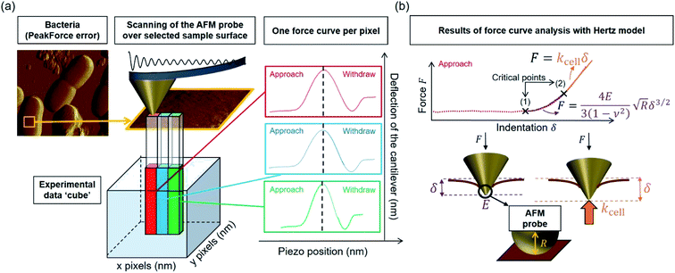 |
| | Fig. 1 (a) Representation of experimental data ‘cube’ collected by Atomic Force Microscopy (AFM) operating in PeakForce tapping mode; (b) illustration of the procedure according to which cell spring constant (kcell) and Young modulus (E) of the cell envelope are retrieved from the analysis of a force versus indentation curve constructed from the corresponding cantilever deflection versus piezo position raw data measured upon approach of the probe to the sample. For the sake of example, the equations that define the dependence of the force F on the indentation δ refer here to the Hertz model in sphere/plane geometry without Dimitriadis correction (in purple the non-linear deformation regime, and in orange the linear compliance component). The Poisson ratio is denoted as ν (=0.5). R corresponds to the radius of the hemi-spherical AFM probe apex (20 nm in this study). The critical points (1) and (2) stand for the AFM probe-to-sample contact point (CP) and for the onset of the linear compliance regime, respectively. The physical meaning of the indentation δ is further illustrated in the schemes both for the non-linear and linear domains of the force curve. See text for details. | |
The major difficulty for an adequate application of these models, independently of their underlying approximations, is a clear identification of the non-linear indentation domain in the force curve and of the onset of the compliance regime (Fig. 1b). Such identification goes in pair with a proper definition of the contact point34 (CP in short, hereafter denoted as the critical point (1), see Fig. 1b) between the AFM probe and the sample surface within the force versus indentation curve representation. Unambiguous positioning of the CP is generally not an easy task as it is inferred from both probe deflection and vertical position of the piezoelectric. As a result, it is impaired by the action of probe–sample intermolecular forces (e.g. hydrostatic, electrostatic or van der Waals) and by the low signal-to-noise ratio in the domain of the force curve where probe and sample are close to contact. Evaluation of the critical indentation value marking the transition between non-linear and linear regimes (denoted hereafter as the critical point (2), see Fig. 1b) is less prone to controversy: the most straightforward method for that purpose is by ‘visual’ inspection of the data, but then results may significantly differ from one investigator to another. The suitable option for locating the aforementioned transition and contact point is thus the elaboration of a reliable and automated data-treatment strategy. To the best of our knowledge, this possibility is currently not offered by PeakForce data processing proposed by AFM manufacturers (and by the often adopted visual, ‘point and shoot’ determination of contact point), not to mention the limits of such processings for treating tens of thousands force curves at once and for delivering associated spatial maps and distributions of relevant nanomechanical parameters.
In order to automatize mechanical data treatment, several solutions have been elaborated for a variety of samples.22,31,35–46 These solutions refer mostly to the analysis of force curves acquired in force volume (FV) mode, which – unlike the PeakForce tapping mode – results in a more limited amount of data (few thousands force curves collected over a 500 × 500 nm2 scanned surface area) and thus in a reduced resolution of the spatial maps derived for the physical parameters of interest. The fast force volume (FFV) mode offers a better performance than the FV mode in terms of acquisition speed and amount of measured force curves, but still it does not seem to compete with PeakForce Tapping (PFT) solution. Indeed, Efremov et al.,45 with the AFM settings operational in their work, argue that ‘the acquisition time was ∼10 min for FV (32 × 32 points), ∼4 min for FFV (64 × 64 points), and ∼10 min for PFT (256 × 256 points, but only 64 × 64 points array was saved due to the hardware limitations)’. Accordingly, from these data one can estimate that a FFV measurement delay of ca. 15 min corresponds to ca. 128 × 128 force curves. In other words, one requires 5 min extra FFV acquisition time as compared to PFT to collect 4 times less force curves. In addition, FV and FFV solutions rarely interpret the linear compliance regime of the force curves as measured for e.g. bacterial cells.23,28,30 The methodology proposed by Chang et al.6 is of particular interest due its simplicity in terms of implementation, and its robustness for the derivation of CP. The main underlying idea consists in exploiting a significant signal-to-noise ratio domain of the force curves rather than that corresponding to the indentation regime located in the direct vicinity of the contact point where this ratio is necessarily low. Accordingly, Chang et al.6 developed and successfully tested a novel algorithm for automated contact point detection through the analysis of 64 × 64 force curves recorded by AFM in force–volume mode.6 Though efficient, the approach solely integrates Hertzian mechanics and thus discards the evaluation of the additional critical point (Fig. 1b) marking the transition between linear and non-linear indentation regimes (Fig. 1b), an operation that is however required for bacterial cells.23,28 Aware of this limitation, Chang et al.6 emphasized that efforts were further needed to extent their approach for a proper treatment of more complex scenario where non-linear and linear changes of the force with increasing indentation are measured. In this report, we propose a data treatment methodology that addresses the aforementioned limitations of previous methods while allowing for a clear and automated definition of the critical contact point and of the transition point between non-linear deformation regime and compliance domain (Fig. 1b). This step is all the more crucial as any error in the identification of these two critical points may lead to significantly biased maps of cells Young modulus and stiffness. Additional strengths of the here-developed numerical data treatment are its capacity (i) to handle a large amount of data, a feature that is mandatory for the interpretation of force curves collected in PeakForce tapping mode, (ii) to easily test the suitability of different mechanical models (here, the Hertz31 and Sneddon46 models, corrected or not for effects of finite sample thickness) in reproducing the non-linear dependence of the force on indentation in the non-linear deformation regime, and (iii) to easily exclude, if necessary (e.g. when working on eukaryotes), the treatment of the linear compliance regime that is relevant to turgescent cells. The performance of our numerical algorithm, implemented in the form of a MATLAB program run with a regular laptop, was tested on more than hundred thousands of force curves collected on Escherichia coli cells, the completion of the analysis being achieved after only ca. 25 minutes for treatment of 65536 force curves acquired on a 500 × 500 nm2 cell surface area.
The article is organized as follows. First, we provide a description of the Escherichia coli cells selected for the AFM PeakForce measurements. We then present the key steps of our algorithm together with the physical models adopted for analysis of data measured on bacteria, i.e. the Hertz31 and Sneddon46 contact mechanics formalisms corrected (or not) for finite sample thickness, and the evaluation of cells surface stiffness from exploitation of the linear compliance regime. Finally, illustrative force curves data are analyzed according to our numerical data strategy using the MATLAB home-made program, leading in fine to the elaboration of resolved spatial maps of cell Young's modulus, cells stiffness and critical indentation at the transition between non-linear and linear deformations of the biological sample. Given the approximations underlying the applicability of the Hertz and Sneddon models – that are classically adopted for the lack of better tractable alternatives – to analyse nanomechanics of biological samples, a comparison of their respective performance is here further reported and thoroughly discussed.
2. Materials and methods
2.1 Bacterial culture
AFM force curves were measured on the deep rough Escherichia coli bacterial strain BW25113 (rod-shaped cells with 700 to 800 nm diameter and 2 to 3 μm length47) obtained from the Coli Genetic Stock Center of Yale University, USA,48–53 and selected here for testing the performance of our automated treatment of force curves. For the experiments, cells were streaked from glycerol stocks on LB agar plates. Overnight initial pre-cultures were obtained by inoculating single cell colonies in 4 mL of M9 minimal medium (composition per liter: MgSO4 1 mM, CaCl2 0.1 mM, thiamine 10 μg mL−1, 2 g L−1 glucose, proline 20 μg mL−1, uridine 25 μg mL−1) and incubation at 37 °C under 150 rpm agitation. The next day, 1 mL precultures volume was introduced in 100 mL of M9 minimal medium, incubated at 37 °C and 150 rpm until OD600 nm reached 0.4–0.6. Then, cells were washed twice by centrifugation–resuspension (5000 × g for 8 min) in 10 mM KNO3 aqueous solution and adjusted to OD600 nm 0.4 prior to experiments. The deep rough mutant selected in this work is decorated by lipopolysaccharides (LPS) lacking the O-antigen part,53 with a resulting LPS length of ca. 4 nm as independently confirmed by detailed electrohydrodynamic analysis of BW25113 electrophoretic properties.51
2.2 AFM PeakForce measurements
Drops of cell suspension obtained as described above were first deposited on cleaned borosilicate glass slide previously covered with a layer of polyethyleneimine (PEI) (Sigma, Mw = 750000 g mol−1), a cationic polymer, upon immersion in 0.1% PEI solution during 30 min. Then, the glass slide was rinsed with 1 mM KNO3 solution to remove unbound or loosely bond bacteria from the surface. The living bacteria fixed on the surface were then maintained in a 1 mM KNO3 environment during AFM experiments performed at ambient temperature and natural pH. Measurements were then conducted with a FastScan Dimension Icon with Nanoscope V controller (Bruker) operating in PeakForce tapping mode in fluid medium. This mode has the advantage to provide simultaneously both cell surface images with ca. 20 nm resolution (size of the hemi-spherical AFM probe apex) and loading force measurements as a function of the AFM probe-to-cell surface separation distance (Fig. 1a). The adopted AFM probes were NPG Silicon Nitride probes (NPG-10, Bruker corporation) with cantilever spring constant of 0.40 ± 0.2 N m−1 determined as detailed elsewhere.54 Force curves were measured systematically at the apex area of the bacterial cells and not at their periphery so as to minimize convolution between probe geometry and sample surface topography. Prior to each experiment, the deflection sensitivity was determined from measurement on a hard substrate and the thermal tuning method was adopted for fine evaluation of the cantilever spring constant. Force versus indentation curves were then derived from raw data (i.e. cantilever deflection [nm] versus vertical piezo position [nm]) collected during the approach of the AFM probe to the bacterial surface (see details in Section 3). These raw AFM data were recorded pixel-by-pixel at the apex of the cell with 500 nm scan size at 1 Hz scan rate and probe velocity displacement of 1 μm s−1, which corresponds to 256 × 256 local force measurements on the investigated cell surface area. As a result, 65536 force curves were generated on 500 × 500 nm2 surface area of a single cell, which asks for a rapid and robust numerical tool to handle their automatic analysis done according to the methodology detailed below. Reproducibility of the obtained data was addressed upon repeating the experiments on several bacteria issued from one or different colonies. Completion of the analysis of the force curves acquired on a single cell was achieved after 25 minutes at most with use of a computer whose technical specificities are: Intel® Xeon® CPU E3-1505M v5 @ 2.80–2.81 GHz and installed RAM memory of 32.0 GB with an operating system of 64 bits. The algorithm reported in this work can be easily implemented in a computer cluster.
2.3 Non-linear deformation models and corrections for finite thickness of the probed sample
The formalism implemented in the algorithm which is detailed below and is dedicated to PeakForce data treatment, refers to the Hertz or Sneddon model (which is specified by the user in the code), corrected or not for effects of finite sample thickness (option also specified by the user), for interpretation of the non-linear deformation regime achieved at sufficiently small indentations (Fig. 1). This section briefly recalls the fundaments of each model and details how they are fully integrated in the procedure elaborated for e.g. the automatic search of the probe-to-sample contact point.
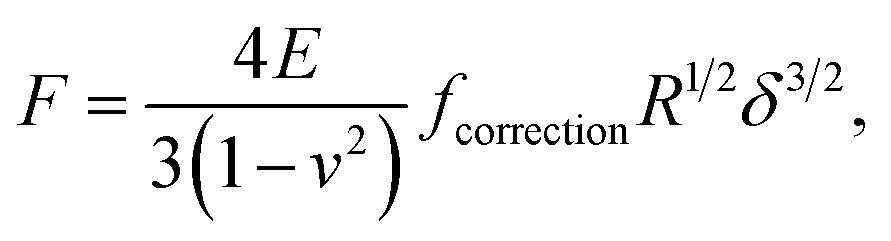
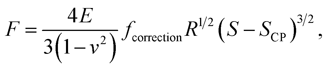
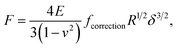
2.3.1 Hertz model and Dimitriadis correction. Unlike Chang et al.6 who considered the standard Hertz model31 for analysis of the non-linear deformation domain of the force versus indentation curves, the algorithm detailed in this paper integrates the factor formulated by Dimitriadis et al.36 which corrects the classical Hertzian formulation of the force for the effect of the finite thickness of the probed sample. In turn, the relation between the force F and the indentation δ is defined for a spherical indenter of radius R by (eqn (1)):| |
 | (1) |
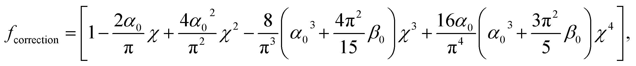
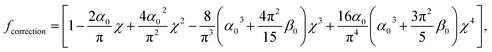
where ν is the Poisson coefficient with value 0.5 (i.e. bacteria samples are viewed as incompressible materials36,55,56), R is the radius of the hemi-spherical AFM probe apex, and fcorrection is the Dimitriadis' correction factor expressed by (eqn (2)):| |
 | (2) |
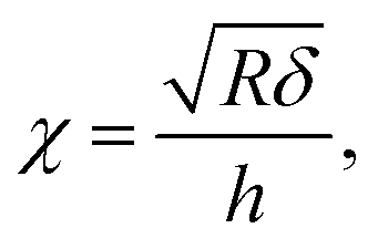
with χ defined by| |
 | (3) |
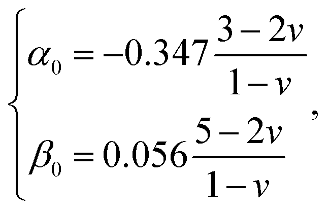
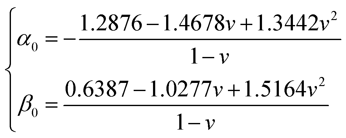
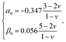
and h refers to the height of the sample (typically 800 nm for a bacterium cell, the value adopted in this study). The constants α0 and β0 involved in eqn (2) depend on the Poisson coefficient ν and differ for situations where sample is ‘not bonded’ or ‘bonded’ to the underlying substrate. In the former case, we have (eqn (4)):| |
 | (4) |
whereas in the latter situation, expressions become (eqn (5)):| |
 | (5) |
It is stressed that the expression of the correction factor fcorrection by Dimitriadis et al. (2002) is valid for h ≥ 0.1R and δ ≪ h,36 conditions that are applicable under the PeakForce acquisition conditions for bacterial cells with probe radius R = 20 nm (mean δ is of the order of ∼50–60 nm, see Section 4 and Fig. 9, and h is ca. 800 nm). In the limit fcorrection → 1, eqn (1) reduces to the standard Hertz expression. A key advantage of Dimitriadis' expression is that, depending on sample properties, the analysis of the force curves based on eqn (1) may lead to a refined estimate of Young modulus and, in turn, to a better evaluation of the compliance regime via explicit account of the sample height (eqn (2)). Eqn (1) is valid for low indentations δ compared to probe curvature radius R (δ ≪ R). This equation further approximates the sample as a linear elastic and isotropic material, which is an obvious and well-recognized approximation for bacterial cell envelopes.57 For the lack of better, this model is however widely used in AFM literature, and our purpose is here to test its applicability for capturing or not the power-law indentation-dependence of forces measured by PeakForce tapping mode on bacteria. Given these elements, eqn (1) may be rewritten in terms of the contact point CP (eqn (6)):
| |
 | (6) |
with
S the probe-to-sample separation distance (nm) and
SCP the value taken by
S at the contact point where
F = 0. In practice,
SCP deviates from the intuitively anticipated 0 value due to effects of short-range AFM probe–sample interactions that contribute to signal noise.
Eqn (6) makes explicit the requirement to properly estimate the magnitude of
SCP for an adequate evaluation of the Young modulus from force
versus indentation curve analysis. It is recalled that the radius of the AFM probe chosen in this work is orders of magnitude lower than the curvature of the cell surface, which guarantees the validity of a sphere (probe) to planar surface (cell) indentation configuration despite of the cylindrical shape of the bacteria.
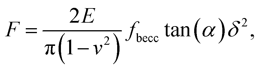
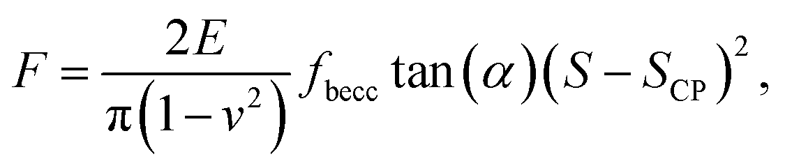
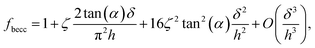
2.3.2 Sneddon model and bottom effect cone correction. For indentations δ exceeding the tip radius R, Young moduli are classically extracted from force curves measurements by use of Sneddon model.46 The latter relates the load force to indentation depth for a conical shape indenter in an elastic and isotropic material according to:46,58| |
 | (7) |
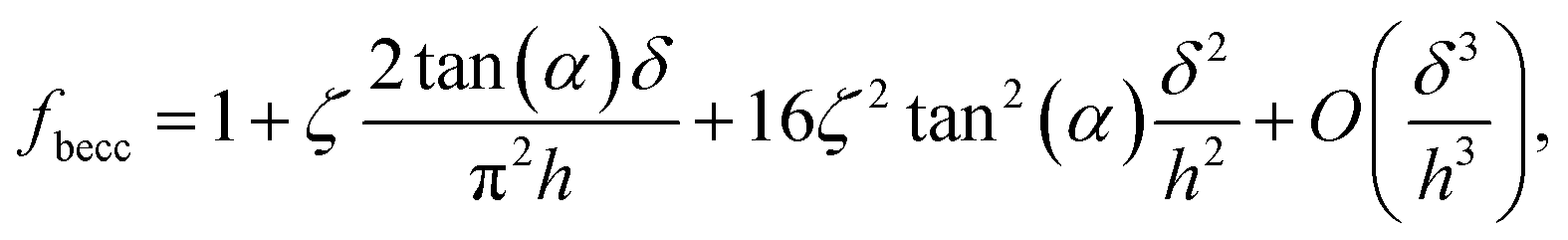
where α represents the half opening angle of the cone (here 17.5°) and fbecc is the bottom effect cone correction (becc, in short) that corresponds to the counterpart of the Dimitriadis factor fcorrection in the sphere-plane indentation geometry. Similarly to the factor fcorrection, the corrective scalar fbecc is defined by two expressions depending on whether the sample is bonded or not bonded to the underlying substrate, namely:| |
 | (8) |
with ζ = 1.7795 and ζ = 0.388 applying to adherent or non-adherent cells, respectively. Eqn (7) can be recast in the form:| |
 | (9) |
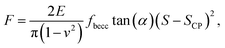
where we made explicit the dependence of F on SCP, similarly to eqn (6). It is stressed that the equivalent of eqn (7) for a pyramidal indenter, as reported by Bilodeau,59 also displays a load force that varies according to the power law ∼ δ2. In turn, it is virtually impossible to discriminate between conical and pyramidal shape effects on force curves from the analysis of the dependence of F on indentation δ: consideration of both geometries will necessarily lead to equivalent data fitting quality, with a resulting Young modulus that simply differs according to a constant multiplier.
3. Description of the algorithm
Fig. 2 reports a flowchart that details step-by-step the here-proposed algorithm for treatment of the force curves. To summarize, the automated processing of AFM PeakForce curves leading to evaluation of spatially resolved Young modulus and cell spring constant (or stiffness) of biological samples proceeds according to five main actions: the extraction of the raw data (i.e. 65536 curves for 256 × 256 pixels covering a 500 × 500 nm2 scanned cell surface area) (Fig. 2, STEP 1), the establishment of a baseline correction for each extracted curve (Fig. 2, STEP 2), the determination of their respective linear (compliance) domain (Fig. 2, STEP 3) and the subsequent calculation of the associated cell spring constant kcell (Fig. 2, STEP 4), and finally, the evaluation of Young's modulus from each measured force curve (Fig. 2, STEP 5). Each step is thoroughly discussed in the following sections.
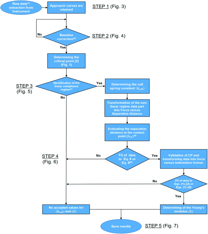 |
| | Fig. 2 Flowchart detailing the program. 1Raw data correspond to cantilever deflection versus piezo position (Zsensor). 2The test ‘Yes’ or ‘No’ is based on the minimal amount of data required for proper definition of the baseline, set here to 30% of the total number of measured points per force curve. 3This ‘Yes’ or ‘No’ test is based on whether an imposed criterion evaluating the quality of the linear regression of the data within the compliance regime is satisfied or not. 4This first evaluation of SCP makes use of a signal-to-noise criterion. 5The fit is performed upon adjustment of SCP (initial guess value derived in the previous step) and of the Young modulus E (initial guess value to be updated according to the type of sample considered, typically 1 MPa for bacterial cells). This fit is performed to achieve a clear identification of the range of S values corresponding to the non-linear deformation domain of the force curves. | |
3.1 STEP 1: raw data extraction from Bruker instrument
The raw AFM data are first extracted from the PeakForce Curve file (.PFC format) generated by the Bruker instrument, with the help of the MATLAB ‘utilities’ toolbox delivered by the Bruker company. Accordingly, right from the beginning of the data process and all during data treatment (i.e. from raw data extraction to generation of outputs and post-processing) work is continuously performed in MATLAB® environment (version: 9.0.0.370719 (R2016a)), starting with a ‘cell array’ where the first column corresponds to the name given by the user to the experiment with specification of the amount of measured force curves; the second and third columns pertain to the approach curve data, i.e. the AFM probe deflection (in nm) versus the piezo position (denoted as Zsensor in nm) (Fig. 3a). The onset of the retraction force curves (i.e. measured when the probe moves away from the sample surface) is marked by a maximum in the deflection versus piezo position (red cross in Fig. 3a). As the analysis is intended for the force curves collected upon approach of the probe to the sample surface, the data corresponding to Zsensor values above that maximum were not considered in the following treatment steps.
 |
| | Fig. 3 Illustration of STEP 1: extracting the raw data (in panel (b), baseline correction was further applied). | |
Fig. 3b further illustrates that data with Zsensor values slightly less than the maximum in piezo position were not subjected to further analysis since they correspond to a transition between the approach and the withdraw phases and, as such, they involve a complex interplay between the probe-to-surface interactions of interest and cantilever dynamics. To put it in a nutshell, data corresponding to piezo positions where the derivative of the signal increases or remains constant with increasing Zsensor were retained for subsequent numerical treatment (Fig. 3b). The second step consists in defining properly a baseline.
3.2 STEP 2: establishment of a baseline correction
Defining a proper baseline is a key element for any data interpretation. In practice, force curve measurements may be affected by noise and thermal drift, which results in steady changes of the force applied by the instrument on the sample. As a consequence, a non-zero probe deflection is measured in the pre-contact region between the probe and the sample surface. Also, the hydrodynamic force due to viscous friction of the cantilever with the liquid results in a drag that contributes to baseline deviation. Magnitude of the latter depends on, among other parameters, probe velocity, damping effect or type of force measurements performed. In the program, an option allows the user to select a number of points to be considered for defining the baseline. This number may vary from one experiment to another depending on the nature of the sample considered and on the liquid composition adopted for the experiments. A linear regression of the selected data is then applied as indicated in Fig. 4a and the obtained expression is then subtracted to the complete set of deflection data (Fig. 4b). There are literature reports where baseline is fitted according to a non-linear procedure upon correction of the instrumental response force versus time.60 For the data of interest in this work, our adopted linear baseline correction procedure is similar to that employed by Efremov et al.45 and the typical pattern of our approach and retraction force curves significantly differs from that given by Ortega-Esteban et al.60 (Fig. 2c therein).60 Our baseline correction procedure was applied to each force curve measured over the sample surface. The next step aims at determining the cell spring constant or stiffness.
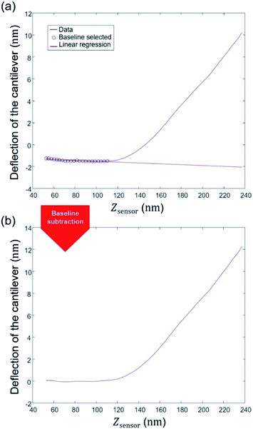 |
| | Fig. 4 Illustration of STEP 2: establishment of a baseline correction. | |
3.3 STEP 3: determination of the cell spring constant (cell stiffness)
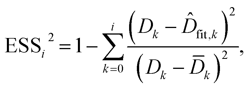
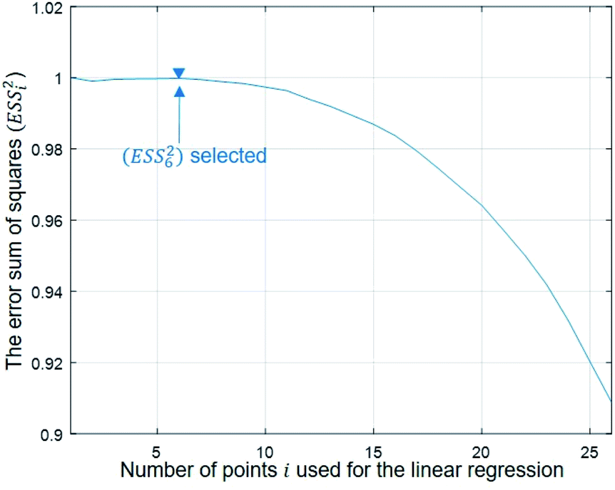
To evaluate the cell stiffness denoted as kcell (Fig. 1b), the piezo position marking the frontier between the Hertz regime and the linear compliance regime needs to be clearly identified. For that purpose, several linear regressions of the tip deflection (hereafter denoted as D) versus piezo position (Zsensor) data are performed over distinct ranges of Zsensor values in the interval [Zsensor,i; Zsensor,0] where Zsensor,0 corresponds to the largest piezo position at the edge of the compliance regime and Zsensor,i < Zsensor,i−1 the indexed piezo position where i is iterated from 1 to N and N is lower than the total number of measured data points (Fig. 4). The error sum of squares ESS2 is then computed for each linear regression (indexed i) over the range [Zsensor,i; Zsensor,0] (range of deflection values [Di; D0]) and the corresponding ESSi2 is defined here by eqn (10):| |
 | (10) |
where ![[D with combining macron]](https://www.rsc.org/images/entities/i_char_0044_0304.gif) k is the average of the Dk, and
k is the average of the Dk, and ![[D with combining circumflex]](https://www.rsc.org/images/entities/i_char_0044_0302.gif) fit,k is the estimated value of the deflection at Zsensor,k on the basis of the linear regression in the compliance regime. The number N of points and, therewith, the [Zsensor,N; Zsensor,0] range of piezo positions defining the searched linear compliance regime corresponds to a ESS2 value that does not significantly deviate (i.e. by less than 0.1%) from that obtained on the basis of the regression performed over N − 1 points. The further condition imposed when identifying this number N of points is that it should satisfy the inequality N ≥ 5 (Fig. 5). The cell stiffness, kcell, is obtained from the (dimensionless and positive) slope a of the now identified linear compliance regime of the deflection (nm) versus piezo displacement (nm) curve according to eqn (11):23
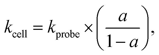
fit,k is the estimated value of the deflection at Zsensor,k on the basis of the linear regression in the compliance regime. The number N of points and, therewith, the [Zsensor,N; Zsensor,0] range of piezo positions defining the searched linear compliance regime corresponds to a ESS2 value that does not significantly deviate (i.e. by less than 0.1%) from that obtained on the basis of the regression performed over N − 1 points. The further condition imposed when identifying this number N of points is that it should satisfy the inequality N ≥ 5 (Fig. 5). The cell stiffness, kcell, is obtained from the (dimensionless and positive) slope a of the now identified linear compliance regime of the deflection (nm) versus piezo displacement (nm) curve according to eqn (11):23| |
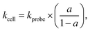 | (11) |
where kprobe (N m−1) is the spring constant of the probe evaluated according to the procedure detailed by Arnoldi et al.28 and Velegol et al.61 The next step of the analysis deals with the estimation of the cell Young's modulus (E) on the basis of Hertz or Sneddon model corrected for the Dimitriadis or becc term (eqn (1) and (2) and eqn (7) and (8), respectively). The relevant range of Zsensor values to be considered for that operation is Zsensor < Zsensor,N and the evaluation of E requires the prior identification of the contact point CP.
 |
| | Fig. 5 Dependence of the error sum of squares on the number of points used for regression (see text for details). | |
3.4 STEP 4: determination of the Young's modulus for a given probed pixel of the cell surface
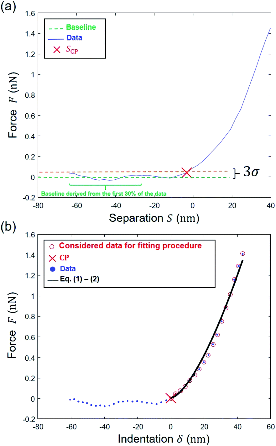
The data are now transformed into force (nN) versus separation distance (nm) curve format according to Hook's law:where we recall that D is the deflection [nm], S is the separation distance [nm] and Z = Zsensor is the piezo displacement [nm] satisfying the inequality Zsensor < Zsensor,N. In line with the strategy adopted by Chang et al.6 a range of S values to be further considered for data fitting to eqn (6) or eqn (9) is first determined by choosing ‘arbitrarily’ an initial guess value for SCP on the basis of a signal-to-noise ratio-based criterion. In detail, an estimation of that noise level in the pre-contact region (baseline domain) is done by averaging the force values measured in that region and by evaluating the associated standard deviation (denoted as σ, Fig. 6a). This operation is performed by considering the 30% fraction of the data that corresponds to the lowest separation distance S values recorded (Fig. 6a). Then, the searched SCP guess value is that for which the force corresponds to the mean force value plus 3 times σ, the value ‘3’ being classically adopted for evaluation of noise in e.g. spectroscopic data. We verified that defining the SCP guess value as that where the force is the mean force value plus 4 or 5 times σ does not modify the outcome of the nanomechanical end results (Fig. S1†).
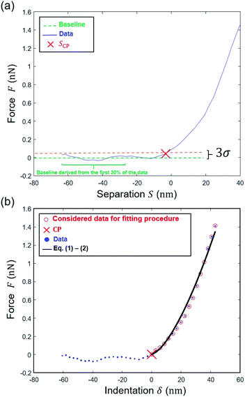 |
| | Fig. 6 Determination of the Young's modulus for a given pixel on the basis here of Hertz–Dimitriadis model. (a) Estimation of SCP by finding the point above the 3σ threshold level; (b) determination of the region where a first regression is performed to find the ‘correct’ CP and then data are fitted to the Hertz–Dimitriadis model for determination of the Young's modulus (corresponding ESS2 = 0.99). | |
The experimental force versus separation distance data corresponding to S varying between the SCP value previously determined and the onset of the linear compliance regime are then fitted to the Hertz–Dimitriadis expression (eqn (6)) with α0 and β0 defined by eqn (5), or by the Sneddon–becc expression (eqn (9)), recalling here that the deposited Escherichia coli cells are considered ‘bonded’ to the PEI substrate. The variables SCP and E are here adjusted using mean-square Levenberg–Marquardt regression procedure (Fig. 6b). The obtained SCP solution is subsequently used to transform the S range into indentation range via δ = S − SCP (Fig. 6b). The so-obtained force versus indentation curves are then fitted to eqn (1) and (2) or eqn (7) and (8) with adjustment of the Young's modulus E (the latter is the ‘true’ modulus, i.e. obtained upon consideration of the non-linear domain properly scaled to a CP where separation distance is rigorously zero). The quality of the theoretical reconstruction of the force curve by means of eqn (1) and (2) or eqn (7) and (8) is estimated by computing the error sum of squares (ESS2) defined by eqn (10) where the deflection D is replaced by the indentation δ. If ESS2 is less than a prescribed value specified by the user in the range 0.9–0.99, the elastic modulus (E) is rejected and so is the corresponding force curve (and the associated kcell value).
3.5 STEP 5: saving the results for each probed pixel of the cell surface
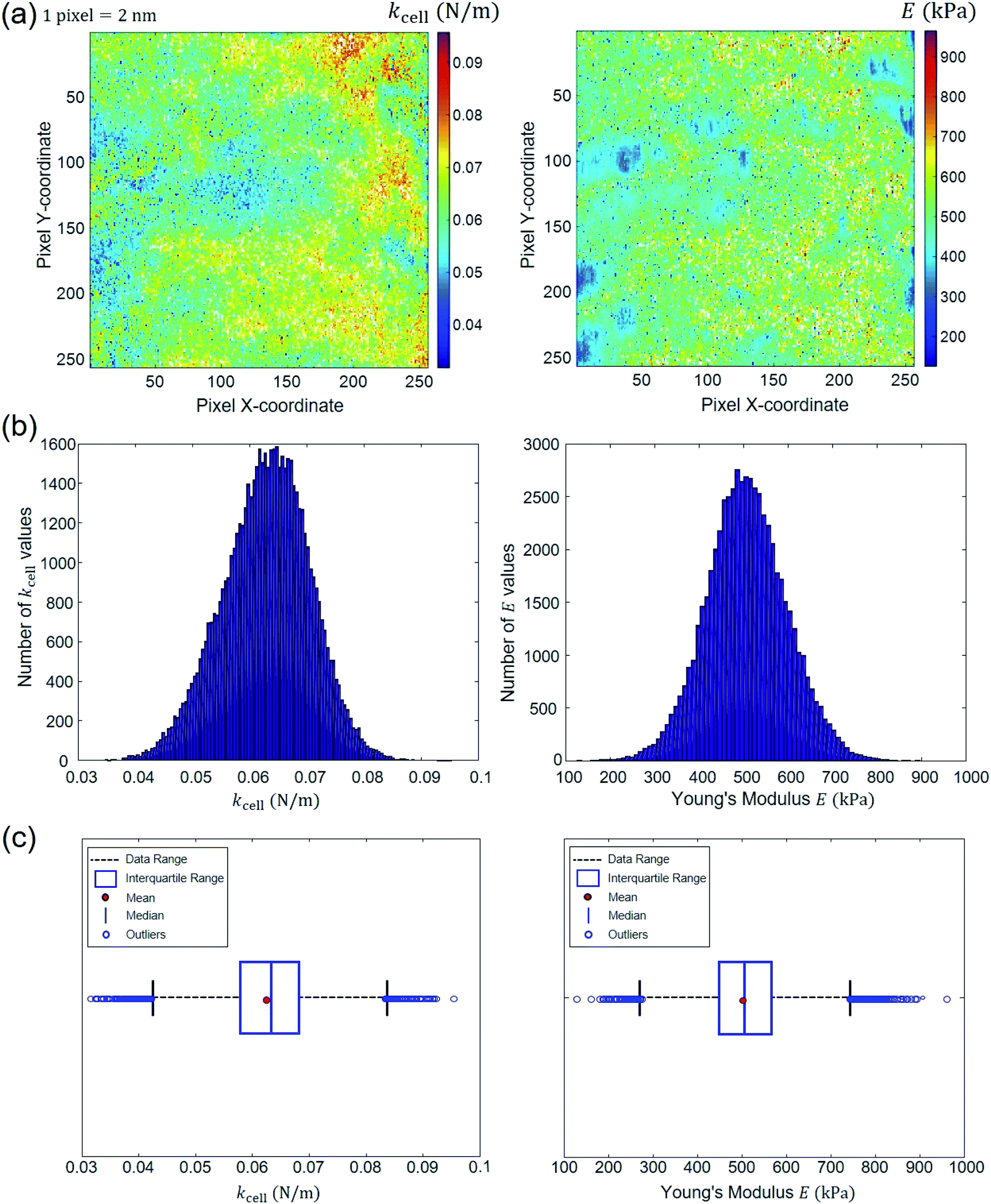
All different STEPS of the algorithm detailed above are saved in a MATLAB ‘cell array’. This provides the possibility to post-process the results pixel by pixel. In particular, the evaluation of the Young's modulus (E) and the cell spring constant (kcell) pertaining to each pixel of the scanned cell surface area makes it possible to generate spatial maps of these nanomechanical parameters and to address their homogeneous or heterogeneous distributions depending on samples and measurement conditions. For the specific example adopted in this study to illustrate data treatment methodology, the E (as inferred from Hertz–Dimitriadis or Sneddon–becc formalisms) and kcell maps can be used to infer information on e.g. the spatial distribution of LPS structures at the periphery of the bacterial cells. Another proxy of interest is the critical indentation value δ* marking the transition between non-linear deformation and compliance regimes. We shall further comment on this in Section 4. Following the strategy indicated by the flowchart in Fig. 2, we report in Fig. 7 illustrative spatial maps of E and kcell values derived from analysis of the 65536 force curves (corresponding to 65536 pixels) measured over the 500 × 500 nm2 probed area of the Escherichia coli cells described in Section 2.1. In detail, the E maps given in Fig. 7 are those derived from treatment of the force curves for which the error sum of squares ESS2 associated with data fitting to Hertz–Dimitriadis theory is higher than 0.95. In the given example, these curves represent 92% of the total force curves collected over the scanned cell surface area. The spatially resolved nanomechanical properties of the bacterial cells highlight irregular surface at the nanometer scale and the existence of patches that likely reflect the heterogeneous distribution of lipopolysaccharides all over the probed cell surface area, in agreement with literature.62 The spatial distributions of E and kcell provided in Fig. 7a are further given in the form of histograms (Fig. 7b). Another so-called whisker–box representation of such data is commonly reported in literature for evaluation of statistical dispersion.63 Therefore, for the sake of completeness, this mode of representation is also provided in Fig. 7c. Therein, the left and right borders of the boxes correspond to the 25th and the 75th percentiles denoted as 25Q and 75Q, respectively. The blue bold band at the middle of the box corresponds to the median. The red point within the box is the mean of the data. Finally, the lower (upper) limits of the whiskers representation correspond to the smallest (largest, respectively) E and kcell values minus (plus, respectively) 1.5 times the interquartile range. The data that fall outside the whisker box are called ‘outliers’. The automated force curves processing also provides Young's modulus E and kcell mean values with corresponding standard deviations. For the treated example, the results read as E = 507.07 ± 90.43 kPa and kcell = 0.0629 ± 0.0077 N m−1, which is in line with order of magnitudes typically reported for bacteria.6,23,58 Furthermore, the program estimates median values for the variables of interest, here 505.31 kPa and 0.0633 N m−1 for E and kcell, respectively. The white points on the E and kcell spatial maps are pixels that do not contain information as they correspond to rejected force curves for which quantitative analysis according to Hertz–Dimitriadis model failed. These safe-guards are necessary to avoid over- or mis-interpretation of force curves of poor quality that may bias the representation of cell mechanical properties. Finally, the procedure detailed in this work was applied to polydimethylsiloxane (PDMS) samples with known Young modulus E = 2.5 ± 0.7 MPa provided by Bruker company for calibration purpose (Fig. S2†). The median value derived for E after applying our automated data treatment procedure using Hertz model without Dimitriadis correction (and without consideration of the compliance domain, not applicable for PDMS material) leads to E = 2550.4 ± 207.2 kPa, which is in correct agreement with tabulated value. For samples like PDMS, we emphasize that there is no compliance regime operational, and the flexibility of our software allows treatment of such data after simple deactivation of the numerical module in charge of identifying and treating the compliance part of the approach force curve. In addition, may the Hertz and Sneddon models be inappropriate to properly capture the nonlinear part of the force curves, then more relevant physical equations can be straightforwardly implemented in our code: it is simply an affair of updating the specific subroutine that details the dependence of the force on indentation. As a last element of this section, in Strauss et al.64 focus is given on the contribution of LPS to the approach force curve. In this study, the analysis is performed on the force versus separation distance (S) curves on the basis of the Alexander-de Gennes expression for brush layer compression.64 In turn, the separation distance S in this work refers to the distance between the AFM probe and the cell membrane that supports the LPS layer assimilated to a brush. Apparently, the contact point in their representation is set at the location where the force dramatically increases (kind of hard wall behavior of the ‘rigid membrane’), which putatively refers to the position where the impact of the membrane on the force curves is most easily detectable. The force profile pattern we obtain significantly differs from the one reported by Strauss et al.64 as our profile rather exhibits a continuous increase of the force with approaching/indenting the probe to/in the cell envelope, and we do not observe any discontinuity in the profile, which contrasts with the abrupt increase of the force at the ‘contact point’ detailed by Strauss et al.64 It is stressed that the continuous type of profile we get very well conforms to that recurrently found in AFM work on Escherichia coli, see e.g. the work by Mathelié-Guinlet et al.57 and others14,23,52 where data were collected on Escherichia coli with AFM set up different from that adopted here. We have tried to fit our force profile measured in the nonlinear indentation regime with help of the Alexander-de Gennes expression and the fit quality was dramatic as it is difficult to assimilate a power law dependence to an exponential one. This suggests that the LPS contribution, if present, is less significant than that of the overall elastic cell envelop under our measurement conditions. This motivates our ignoring of the LPS compression contribution.
 |
| | Fig. 7 Outputs of the automated force curves processing. (a) Spatial maps of E and kcell; (b) corresponding histogram distribution; (c) whisker–box plot distributions. These results derive from analysis of typical force curves collected over a 500 × 500 nm2 cell surface area located at the center of bacterial specimen devoid of septum. Data correspond to a processing performed on the basis of Hertz–Dimitriadis formalism and with considering an error sum of squares for the non-linear deformation regime that is above 0.95. See text for details. | |
4. Discussion
We provide here a discussion of the respective merits of Hertz–Dimitriadis and Sneddon–becc formalisms for fitting the non-linear deformation regimes of the experimental force curves and their implications – if any – on the nanomechanical proxies kcell and δ* (the latter corresponds to the indentation value marking the transition between non-linear and linear force versus indentation regimes). We further detail the results obtained with/without account of the finite sample thickness and discuss maps of the nanomechanical cell properties corresponding to different values of the error sum of squares ESS2 (range 0.9–0.99) specified by the user within the procedure adopted for fitting the non-linear deformation regime. Fig. 8 reports the spatial maps of the Young modulus E derived for BW25113 strain from application of Hertz (hereafter denoted as H) and Sneddon (S) models without the contribution stemming from the finite thickness of the sample, i.e. fcorrection and fbecc are set to unity in eqn (1) and (7), respectively. Histograms of E values associated to the maps displayed in Fig. 8 are provided in ESI (Fig. S3).† The results derive from analysis of the force curves in line with an error sum of squares ESS2 that is larger than 99% (Fig. 8a and c) and 95% (Fig. 8b and d). The percentage of force curves (counted with respect to the total amount of 65536 measured curves) corresponding to such ESS2 values is further specified in Fig. 8 for both the H and S models.
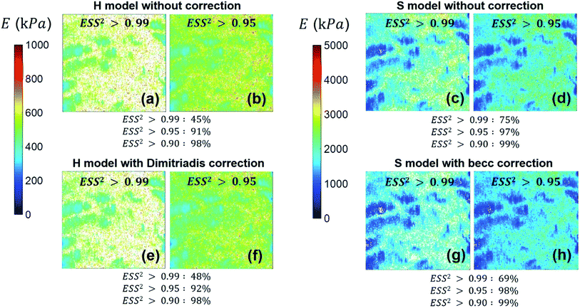 |
| | Fig. 8 Illustrative maps of Young modulus E obtained from analysis of forces curves on BW25113 cells according to Hertz (H) or Sneddon (S) models uncorrected (panels (a–d)) or corrected (panels (e–h)) for the finite thickness of the sample (indicated). Results are displayed for error sum of squares larger than 0.99 and 0.95 (indicated) and the corresponding percent of concerned force curves is further specified. Maps dimensions: 500 × 500 nm2. See text for further details. | |
As expected, the larger the ESS2 value imposed by the user, the least is the number of force curves whose non-linear deformation regime is correctly fitted, and this feature holds irrespective of the type of model (H or S) considered. For a prescribed value of ESS2, there is a larger amount of force data whose dependence on indentation δ gets closer to that subsumed in the S model. This finding coincides with the larger magnitude found for the indentation δ in the non-linear deformation regime analysed according to S model, as compared to the tip radius R. This latter element is reflected by the spatial maps of the critical indentation value termed δ* marking the transition between non-linear deformation and compliance regimes (Fig. 9a–d). Recalling that δ* somewhat depends on the model adopted and on the chosen ESS2 criterion (see Fig. 2), we observe that there is a significant fraction of indentation values δ (<δ*) satisfying the condition δ > R, which favors application of the S model. It should be stressed that proper fitting (depending on ESS2) of the force curves according to S model necessarily spans over a domain of δ values that are lower than R, i.e. the region where this model is supposedly not valid (Fig. 10). Similar argument can be formulated for the applicability of the H model strictly defined for δ ≪ R though data may be reproduced, depending on pixel location, in regime where this inequality is not respected (Fig. 10).
 |
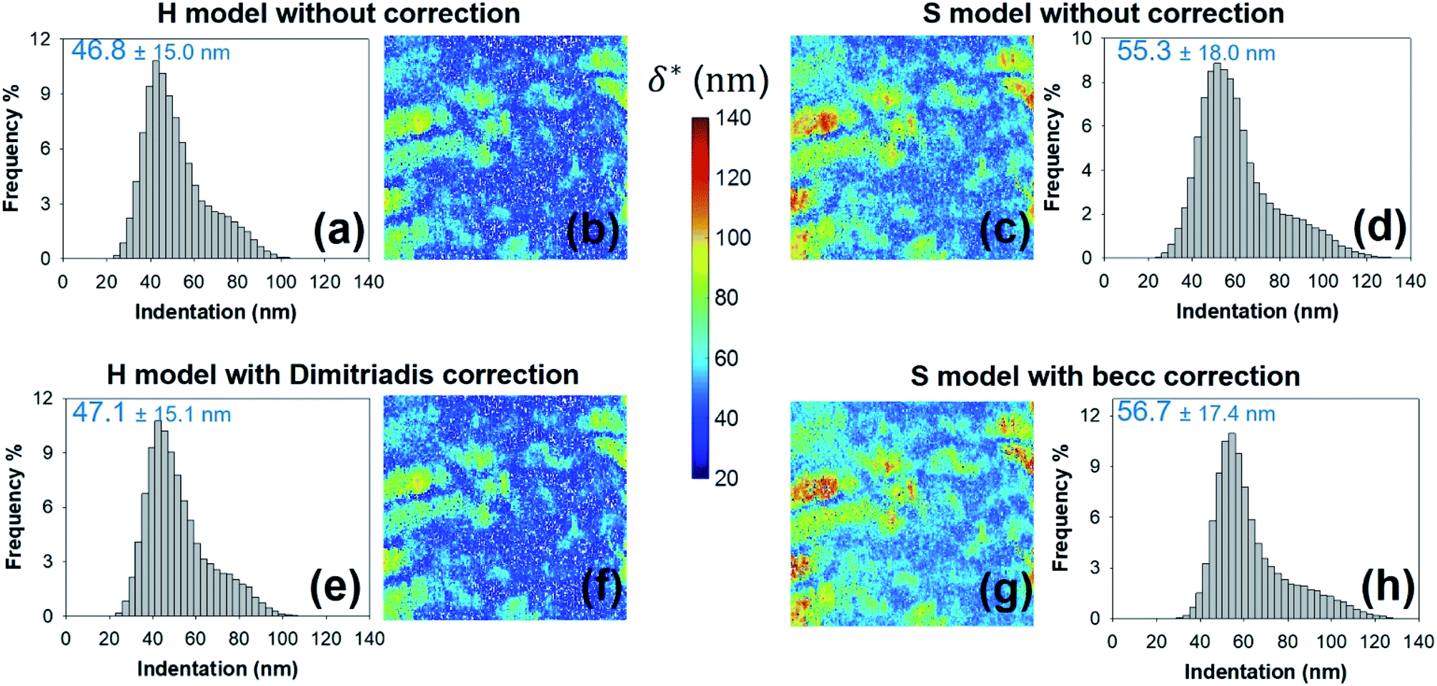
| | Fig. 9 Histograms for – and corresponding maps of – the threshold indentation value δ* derived from force curves analysis according to H and S models with or without correction for finite thickness of the sample (indicated). All results are given for an error sum of squares larger than 0.95. Mean values and associated standard deviations are further specified. Maps dimensions: 500 × 500 nm2. | |
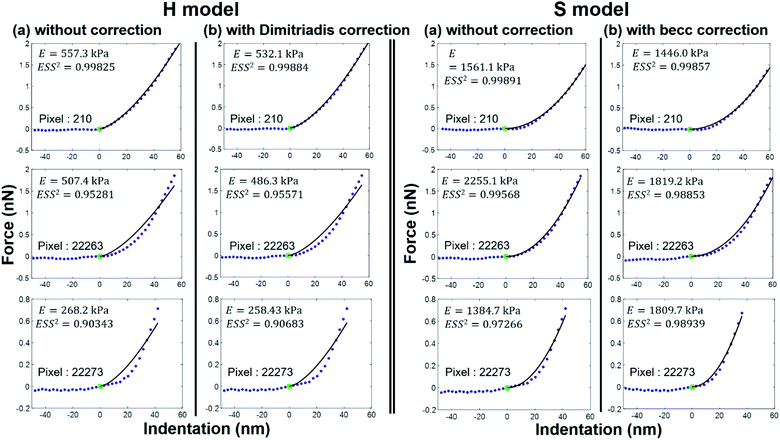 |
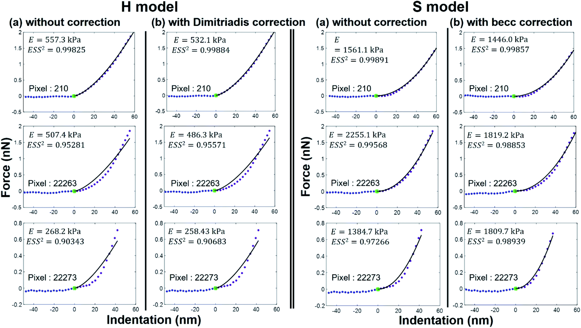
| | Fig. 10 Illustrative comparison between experimental force versus indentation curves (symbols) measured at selected pixel locations (their indexation is indicated) of the cell surface and accompanying theoretical reconstructions (lines) according to H and S models (two columns at the left and right, respectively) with or without correction (column (a) and (b), respectively) for finite thickness of the sample. The value of the E modulus retrieved from analysis is specified together with corresponding ESS2. | |
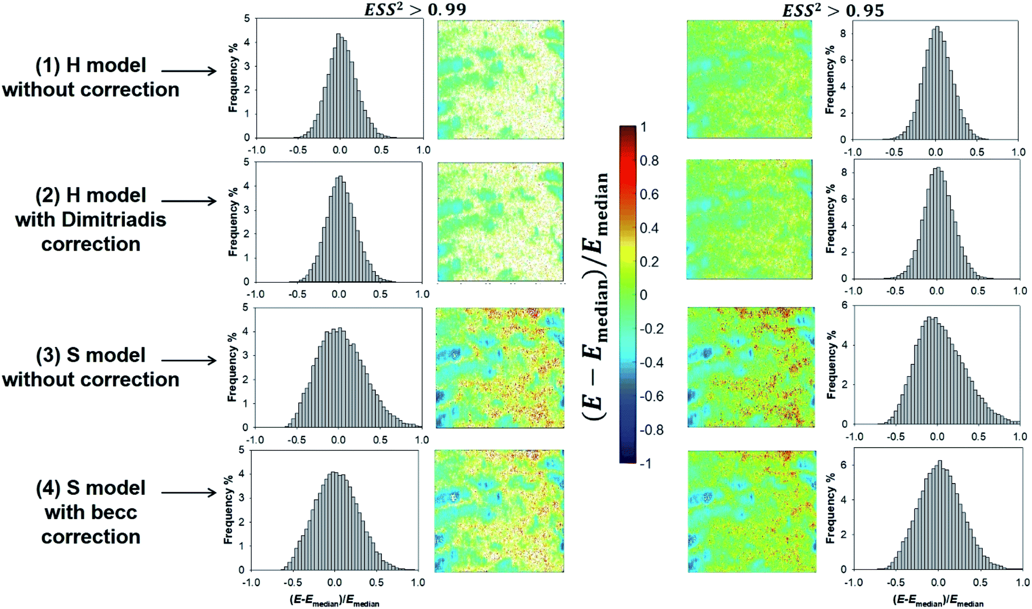
Given the range of indentations achieved in PeakForce mode, none of the H and S model (whose applicability corresponds to extremes of the ratio δ/R) therefore reproduces with full satisfaction (i.e. with ESS2 > 0.99) the ensemble of force curves measured over the whole probed cell surface area (see Fig. 8). Despite this limitation, cell surface heterogeneities revealed by the E and δ* maps (Fig. 8 and 9, respectively) constructed from application of the H and S formalisms are remarkably comparable. This conclusion is particularly clear for ESS2 > 0.95 for which the number of rejected force curves (see Fig. 2 and 8) represents at most 9% of the total number of measured data. It is not straightforward to precisely identify the reasons for the above features given the crude assumptions of isotropic and elastic cell material underlying the obvious (and well recognized) reduced applicability of both the Hertz and Sneddon models for biological samples.57 In particular, eqn (1) and (7) render impossible the differentiated evaluations of the respective elastic and entropic contributions of the outer cell membrane and of the surrounding lipopolysaccharidic cushion (if relevant, see discussion in Section 3.5) or any other surface biomolecules65,66 to the here-obtained effective Young modulus E. Alternatives do exist, as proposed e.g. by Gaboriaud et al.,14 Guz et al.,67 Mercade-Prieto et al.68 for bacteria, brush-like decorated human cells, and yeasts, respectively. In turn, E moduli data should necessarily be viewed as qualitative. Their relative variations with changing composition of the medium (e.g. presence or not of external stressors like nanoparticles)57 remains however very informative provided that the forces curves are systematically measured with the same set of acquisition parameters. These variations may be captured by generating maps and/or distributions of normalized median-centered data, e.g. of the form (E − Emedian)/Emedian with here the Young modulus (Fig. 11) that is most prone to vary with the choice of the selected nanomechanical formalism (E obtained from S model is ca. a factor 3 larger than that derived from H model, see Fig. S3†).
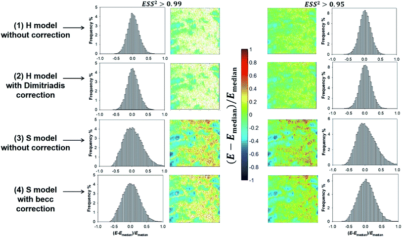 |
| | Fig. 11 Illustrative histograms and associated maps of median-centered Young modulus derived from force curves analysis according to H and S models (two top and bottom lines, respectively) with or without correction for finite thickness of the sample (indicated). Results are provided for error sum of squares larger than 0.99 and 0.95 (two columns at the left and right, respectively). Maps dimensions: 500 × 500 nm2. | |
Fig. 8e–h and 9e–h are the counterparts of Fig. 8a–d and 9a–d for the modulus E and the critical indentation δ* evaluated with account of the finite thickness of the sample (i.e. fcorrection and fbecc in eqn (1) and (7) are now defined by eqn (2) and (8), respectively). Briefly, for bacteria as considered in this work, the Taylor expansions in eqn (2) and (8) do not significantly deviate from unity (because δ/h ≪ 1 and χ ≪ 1) so that the conclusions relative to the impact of ESS2 on E and on the extent of applicability of the H-Dimitriadis and S-becc formulations remain similar to those discussed for situations where fcorrection and fbecc are strictly set to unity. Account of the correction fbecc in the S model leads to filtering of the largest E modulus values, as judged from comparison of Fig. 8c and d with Fig. 8g and h and associated histograms given in Fig. S3.† This property, already identified by Gavara et al.58 originates from the Taylor expanded form of fbecc, and it is lesser marked when analyzing data according to H model corrected by the Dimitriadis factor fcorrection. The distribution in Young modulus (indentation δ*, respectively) obtained from H(-Dimitriadis) model are shifted to lower (larger, respectively) values compared to those evaluated from the S(-fbecc) formalism (Fig. S3,† 8 and 9). Again, the heterogeneous character of the cell surface highlighted by the spatial maps of both E and δ* remain basically similar whether corrections for fine cell thickness are accounted for or not (Fig. 9 and 11).
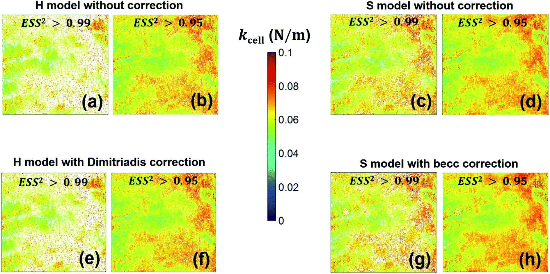
With respect to the nanomechanical proxy kcell, we find that its spatial distribution (Fig. 12) remains similar whether force curves are interpreted according to H or S model. Its magnitude (Fig. S4†) is further essentially independent of the type of model adopted for analyzing the non-linear deformation regime, irrespective of the account or not for sample thickness correction. The only differentiating property is the number of successfully fitted data (or force curve) per class of kcell values that is larger with considering the S model. This is explained by the acceptation of kcell values that is tied to successful analysis of the non-linear deformation regime and corresponding derivation of E modulus (Fig. 8). In addition, the heterogeneity revealed by the distribution in kcell is qualitatively reminiscent of that highlighted by the maps of E and δ* even though differentiated distribution patterns may be detected at various locations of the probed cell surface. The connection between E and kcell is explained by the fact that these two nanomechanical parameters both involve contributions from flexible surface structures located at the bacterial envelope, as evidenced and discussed by Francius et al.23 In particular, cell stiffness is a monotonous function of the turgor pressure and depends on the stretching modulus of the bacterial envelope whose magnitude is intimately determined by the presence of protruding cell surface structures.23,28 This explains why the median values of these nanomechanical proxies as derived over given cell surface areas vary in the same way with changing e.g. cell surface phenotype of a given bacterial strain.23,52 Distinct heterogeneities may however be revealed from maps of E and kcell depending on the nature of the biological system analysed,52 recalling that E particularly pertains to the outer cell envelope and kcell reflects more significantly features of the whole membrane as a result of its dependence on intracellular turgor pressure and cell surface stretching modulus.52
 |
| | Fig. 12 Counterpart of Fig. 8 for the cell spring constant (cell stiffness), kcell. | |
Last, we report in Fig. S5 and S6† maps and histograms of Young modulus generated along the lines detailed in Fig. 2 together with those provided by Bruker Software (offline Nanoscope analysis v1.9, “Run AutoProgram’’ option with baseline correction and indentation steps) on the basis of Hertz and Sneddon models without finite-sample thickness correction (the latter option is not implemented in Nanoscope analysis v1.9) and with unchecking the ‘Adhesion option’. This comparison reveals the following features: (i) heterogeneities of Bruker modulus maps look like those we obtain following our procedure, regardless of the model adopted, (ii) Bruker histograms of Young modulus differ from those we derive, and this difference is most pronounced here when using Sneddon model for data fitting, (iii) the elasticity maps and Young moduli values significantly depend on the range of forces that is arbitrarily selected for batch data analysis by Bruker software, as intuitively anticipated. We report in Fig. S5 and S6† maps collected for a given forces range of 0–2 nN, which provides better fitting than lower force e.g. 0–1 nN (not shown). There are several reasons that possibly explain the above discrepancies: the way the contact point is selected, i.e. ‘Best estimate’ option by Bruker (‘this method emphasizes the minimum force at the contact point while de-emphasizing forces due to noise or interference in the non-contact region, reducing the likelihood that the wrong point is selected’, as detailed by the manufacturer) versus our contact point determination outlined in Section 3.4, the arbitrary choice of the [Fmin − Fmax] interval where fitting procedure is applied to all force curves versus our automated evaluation (iterated for each force curve) of both the non-linear and linear indentation regime boundaries. As additional information, we provide in Fig. S7† histograms of R2 values associated to the goodness of force curves fitting performed with Bruker software. These histograms indicate – regardless of the adopted H or S model (no finite sample thickness included) without account of the linear compliance regime – a fitting that is far less satisfactory compared to the one we provide (our fitting corresponds to the condition ESS2 > 0.95 that applies to 91% and 97% of the whole set of force curves treated according to our algorithm without final sample thickness correction in the H and S models but with proper modelling of the linear compliance regime, see Fig. 8b and d, respectively). We emphasize that our maps, unlike those generated by Bruker software, are constructed upon removal of all force curves that do not satisfy a given prescribed criterion fixed by the user (ESS2 > 0.95 in Fig. S5 and S6, panels (a) and (b)†). This ensures a control over the applicability of the adopted Hertz or Sneddon theoretical equations for a given sample and probed spatial location, and over the statistical coherence of the obtained results. Besides the user-dependent setting of [Fmin − Fmax] interval where data fitting is performed and its implications in terms of evaluation of Young modulus, the above method adopted in Bruker software appeared limited to us for running in batch to analyze tens of thousands of force curves (as required in PeakForce tapping mode). Indeed, there is no reason to arbitrarily set such a transition regime once for all for a full collection of force curves as the precise location of this transition may change from one probed pixel to another due to sample surface heterogeneities. In contrast, our software is designed to properly perform this task. To the best of our knowledge, the above limitations of the Bruker analysis software also hold for Scanning Probe Image Processor Software (SPIP, https://www.imagemet.com/products/spip/). Last, whatever the method chosen for defining the contact point, SPIP and Bruker software analysis remain approximate in their evaluation of Young modulus of bacteria (and all other cells with internal hydrostatic pressure) because of the linear compliance regime they do not rigorously identify and where e.g. Hertz or Sneddon models are blindly applied despite of their invalidity therein. Escape may be found by recording force curves at sufficiently low loading forces to avoid measurement of the compliance regime, albeit at the cost of missing relevant information from exploitation of that compliance regime. It is noted that the incorrect application of the Hertz or Sneddon model within both the non-linear and linear compliance regimes (basically referring to the surrounding cell envelope and the inner cytoplasm compartment, respectively, with obviously different compositions) contradicts the isotropic and homogeneous composition assumptions underlying the validity of these models.
5. Conclusions
We report here an original methodology for the automated processing of tens of thousands of AFM PeakForce curves measured over selected surface areas of biological cells. Data treatment allows for the fast generation of spatially resolved nanomechanical cell properties expressed here in terms of Young modulus and cell stiffness. The interpretation of the force curves is based on two classically adopted theoretical models involving a non-linear deformation of the sample (Hertz or Sneddon formalism corrected or not for finite sample thickness) and a linear compliance regime (Hook's law), both components being required for proper analysis of AFM data collected on turgescent cells like e.g. bacteria. Without loss of generality, the basic principles of the numerical data treatment detailed in this study can be applied to (i) scenario where contact mechanics theories other than those adopted here are required, and (ii) (fast)force–volume data acquisition mode is selected. A major asset of here-reported data processing strategy relates to the speed of the analysis of a large amount of data (typically 25 minutes long treatment of 65536 force curves using standard PC), which allows a full exploitation of AFM PeakForce tapping mode at the single cell level. In addition, the methodology can be easily extended to analysis of data collected at the cell population scale for a robust assessment of reproducibility, or for the identification of sub cellular populations differing with respect to their defining nanomechanical properties. The algorithm further makes it possible to compare the performance of different models for reproducing force curves data measured on biological samples, and the code is flexible enough to be easily adapted for samples whose evaluation of nanomechanical properties does not require consideration of a compliance regime. It is therefore not limited to treatment of data measured on turgescent cells. For bacteria, it is found that the Sneddon model provides an excess of ca. 20% of successfully reproduced force curves as compared to Hertz model. In addition, the spatial maps of the Young moduli and of the threshold indentation values marking the frontier between non-linear and linear deformation regimes, as derived from Hertz and Sneddon models corrected or not for sample thickness, display similar heterogeneities of the probed cell surface.
Conflicts of interest
The authors declare no competing interest. There are no conflicts to declare.
Acknowledgements
The homemade MATLAB code and the presented AFM data are available upon request. This research did not receive any specific grant from funding agencies in the public, commercial, or not-for-profit sectors.
References
- F. Y. Dufrêne, D. Martinez-Martin, I. Medalsy, D. Alsteens and D. J. Müller, Multiparametric imaging of biological systems by force-distance curve-based AFM, Nat. Methods, 2013, 10, 847–854 CrossRef PubMed.
- L. Ressier and V. Le Nader, Electrostatic nanopatterning of PMMA by AFM charge writing for directed nano-assembly, Nanotechnology, 2008, 19, 135301 CrossRef CAS PubMed.
- A. Sethuraman, M. Han, R. S. Kane and G. Belfort, Effect of surface wettability on the adhesion of proteins, Langmuir, 2004, 20, 7779–7788 CrossRef CAS PubMed.
- A. Beaussart, D. Alsteens, S. El-Kirat-Chatel, P. N. Lipke, S. Kucharikova, P. Van Dijck and Y. F. Dufrênes, Single-molecule imaging and functional analysis of Als adhesins and mannans during Candida albicans morphogenesis, ACS Nano, 2012, 6, 10950–10964 CrossRef CAS PubMed.
- S. El-Kirat-Chatel, A. Beaussart, S. Derclaye, D. Alsteens, S. Kucharíkova, P. Van Dijck and Y. F. Dufrêne, Force nanoscopy of hydrophobic interactions in the fungal pathogen Candida glabrata, ACS Nano, 2015, 9, 1648–1655 CrossRef CAS PubMed.
- Y.-R. Chang, V. K. Raghunathan, S. P. Garland, J. T. Morgan, P. Russel and C. J. Murphy, Automated AFM force curve analysis for determining elastic modulus of biomaterials and biological samples, J. Mech. Behav. Biomed. Mater., 2014, 37, 209–218 CrossRef CAS PubMed.
- M. Ornatska, K. N. Bergman, M. Goodman, S. Peleshankoab, V. V. Shevchenko and V. V. Tsukruk, Role of functionalized terminal groups in formation of nanofibrillar morphology of hyperbranched polyesters, Polymer, 2006, 47, 8137–8146 CrossRef CAS.
- M. Tomitori and T. Arai, Tip cleaning and sharpening processes for noncontact atomic force microscope in ultrahigh vaccum, Appl. Surf. Sci., 1999, 140, 432–438 CrossRef CAS.
- C. A. J. Putman, K. O. Van der Werf, B. G. De Grooth, N. F. Van Hulst and J. Greve, Tapping mode atomic force microscopy in liquid, Appl. Phys. Lett., 1994, 64, 2454 CrossRef CAS.
- A. J. Weymouth, D. Wastl and F. J. Giessibl, Advances in AFM: seeing atoms in ambient conditions, e-J. Surf. Sci. Nanotech., 2018, 16, 351–355 CrossRef CAS.
- M. Radmacher, J. P. Cleveland, M. Fritz, H. G. Hansma and P. K. Hansma, Mapping interaction forces with the atomic force microscope, Biophys. J., 1994, 66, 2159–2165 CrossRef CAS PubMed.
- M. Horimizu, T. Kawase, T. Tanaka, K. Okuda, M. Nagata, D. M. Burns and H. Yoshie, Biomechanical evaluation by AFM of cultured human cell-multilayered periosteal sheets, Micron, 2013, 48, 1–10 CrossRef CAS PubMed.
- K. D. Jandt, Atomic force microscopy of biomaterials surfaces and interfaces, Surf. Sci., 2001, 491, 303–332 CrossRef CAS.
- F. Gaboriaud, M. L. Gee, R. Strugnell and J. F. L. Duval, Coupled electrostatic, hydrodynamic and mechanical properties of bacterial interfaces in aqueous media, Langmuir, 2008, 24, 10988–10995 CrossRef CAS PubMed.
- S. Y. Tee, J. Fu, C. S. Chen and P. A. Janmey, Cell shape and substrate rigidity both regulate cell stiffness, Biophys. J., 2011, 100, L25–L27 CrossRef CAS PubMed.
- F. Pillet, L. Chopinet, C. Formosa-Dague and E. Dague, Atomic force microscopy and pharmacology: from microbiology to cancerology, Biochim. Biophys. Acta, 2013, 1840, 1028–1050 CrossRef PubMed.
- P. N. Danese, L. A. Pratt, S. L. Dove and R. Kolter, The outer membrane protein, antigen 43, mediates cell-to-cell interactions within Escherichia coli biofilms, Mol. Microbiol., 2000, 37, 424–432 CrossRef CAS PubMed.
- M. J. McBride, Bacterial gliding motility: multiple mechanisms for cell movement over surfaces, Annu. Rev. Microbiol., 2001, 55, 49–75 CrossRef CAS PubMed.
- J. Y. Wong, A. Velasco, P. Rajagopalan and Q. Pham, Directed movement of vascular smooth muscle cells on gradient-compliant hydrogels, Langmuir, 2003, 19, 1908–1913 CrossRef CAS.
- L. Craig, M. E. Pique and J. A. Tainer, Type IV pilus structure and bacterial pathogenicity, Nat. Rev. Microbiol., 2004, 2, 363–378 CrossRef CAS PubMed.
- C. T. McKee, J. A. Wood, N. M. Shah, M. E. Fischer, C. M. Reilly, C. J. Murphy and P. Russell, The effect of biophysical attributes of the ocular trabecular meshwork associated with glaucoma on the cell response to therapeutic agents, Biomaterials, 2011b, 32, 2417–2423 Search PubMed.
- D. C. Lin, E. K. Dimitriadis and F. Horkay, Robust strategies for automated AFM force curve analysis-II: adhesion-influenced indentation of soft, elastic materials, J. Biomech. Eng., 2007b, 129, 904–912 Search PubMed.
- G. Francius, P. Polyakov, J. Merlin, Y. Abe, J.-M. Ghigo, C. Merlin, C. Beloin and J. F. L. Duval, Bacterial surface appendages strongly impact nanomechanical and electrokinetic properties of Escherichia coli cells subjected to osmotic stress, PLoS One, 2011, 6, e20066 CrossRef CAS PubMed.
- D. Alsteens, D. J. Muller and Y. F. Dufrênes, Multiparametric atomic force microscopy imaging of biomolecular and cellular systems, Acc. Chem. Res., 2017, 50, 924–931 CrossRef CAS PubMed.
- C. Abadias, C. Serés and J. Torrent-Burgués, AFM in peak force mode applied to worm siloxane-hydrogel contact lenses, Colloids Surf., B, 2015, 128, 61–66 CrossRef CAS PubMed.
- X. Li, Y. Feng, G. Chu, N. Ning, M. Tian and L. Zhang, Directly and quantitatively studying the interaction between SiO2 and elastomer by using peak force AFM, Compos. Commun., 2018, 7, 36–41 CrossRef.
- G. Smolyakov, C. Formosa-Dague, C. Severac, R. E. Duval and E. Dague, High speed indentation measures by FV, QI and QNM introduce a new understanding of bionanomechanical experiments, Micron, 2016, 85, 8–14 CrossRef CAS PubMed.
- M. Arnoldi, M. Fritz, E. Bauerlein, M. Radmacher, E. Sackmann and A. Boulbitch, Bacterial turgor pressure can be measured by atomic force microscopy, Phys. Rev. E: Stat., Nonlinear, Soft Matter Phys., 2000, 62, 1034–1044 CrossRef CAS PubMed.
- L. Beauzamy, J. Derr and A. Boudaoud, Quantifying hydrostatic pressure in plant cells by using indentation with an atomic force microscope, Biophys. J., 2015, 108, 2448–2456 CrossRef CAS PubMed.
- P. Polyakov, C. Soussen, J. Duan, J. F. L. Duval, D. Brie and G. Francius, Automated force volume image processing for biological samples, PLoS One, 2011, 6, e18887 CrossRef CAS PubMed.
- H. Hertz, Ueber die Berührung fester elastischer Körper, J. Reine Angew. Math., 1882, 156–171 Search PubMed.
- K. L. Johnson, K. Kendall and A. D. Roberts, Surface energy and the contact of elastic solids, Proc. R. Soc. London, Ser. A, 1971, 324, 301–313 CAS.
- B. V. Derjaguin, V. M. Muller and Y. P. Toporov, Effect of contact deformations on the adhesion of particles, J. Colloid Interface Sci., 1975, 53, 314–326 CrossRef CAS.
- R. Benitez, S. Moreno-Flores, V. J. Bolos and J. L. Toca-Herrera, A new automatic contact point detection algorithm for AFM force curves, Microsc. Res. Tech., 2013, 76, 870–876 CrossRef PubMed.
- S. L. Crick and F. C. Yin, Assessing micromechanical properties of cells with atomic force microscopy: importance of the contact point, Biomech. Model. Mechanobiol., 2007, 6, 199–210 CrossRef CAS PubMed.
- E. K. Dimitriadis, F. Horkay, J. Maresca, B. Kachar and R. S. Chadwick, Determination of elastic moduli of thin layers of soft material using the atomic force microscope, Biophys. J., 2002, 82, 2798–2810 CrossRef CAS PubMed.
- C. Gergely, B. Senger, J. C. Voegel, J. K. H. Hörber, P. Schaaf and J. Hemmerlé, Semi-automatized processing of AFM force-spectroscopy data, Ultramicroscopy, 2000, 87, 67–78 CrossRef.
- M. J. Jaasma, W. M. Jackson and T. M. Keaveny, Measurement and characterization of whole-cell mechanical behaviour, Ann. Biomed. Eng., 2006, 34, 748–758 CrossRef PubMed.
- D. C. Lin, E. K. Dimitriadis and F. Horkay, Robust strategies for automated AFM force curve analysis-I. Non-adhesive indentation of soft, inhomogeneous materials, J. Biomech. Eng., 2007a, 129, 430–440 Search PubMed.
- K. A. Melzak, S. Moreno-Flores, K. Yu, J. Kizhakkedathu and J. L. Toca- Herrera, Rationalized approach to the determination of contact point in force-distance curves: application to polymer brushes in salt solutions and in water, Microsc. Res. Tech., 2010, 73, 959–964 CAS.
- M. A. Monclus, T. J. Young and D. Di Maio, AFM indentation method used for elastic modulus characterization of interfaces and thin layers, J. Mater. Sci., 2010, 45, 3190–3197 CrossRef CAS.
- L. R. Nyland and D. W. Maughan, Morphology and transverse stiffness of Drosophila myofibrils measured by atomic force microscopy, Biophys. J., 2000, 78, 1490–1497 CrossRef CAS.
- M. Radmacher, Measuring the elastic properties of living cells by the atomic force microscope, in Methods in Cell Biology, ed. P. Bhanu and H. J. K. H. Jena, Academic Press, San Diego, CA, 2002, pp. 67–90 Search PubMed.
- C. Roduit, B. Saha, L. Alonso-Sarduy, A. Volterra, G. Dietler and S. Kasas, OpenFovea: open-source AFM data processing software, Nat. Methods, 2012, 9, 774–775 CrossRef CAS PubMed.
- Yu. M. Efremov, A. I. Shpichka, S. L. Kotova and P. S. Timashev, Viscoelastic mapping of cells based on fast force volume and peakforce tapping, Soft Matter, 2019, 27, 5455–5463 RSC.
- I. N. Sneddon, The relation between load and penetration in the axisymmetric boussinesq problem for a punch of arbitrary profile, Int. J. Eng. Sci., 1965, 3, 47–57 CrossRef.
- R. M. Présent, E. Rotureau, P. Billard, C. Pagnout, B. Sohm, J. Flayac, R. Gley, J. P. Pinheiro and J. F. L. Duval, Impact of intracellular metallothionein on metal biouptake and partitioning dynamics at bacterial interfaces, Phys. Chem. Chem. Phys., 2017, 19, 29114–29124 RSC.
- C. A. Schnaitman and J. D. Klena, Genetics of lipopolysaccharide biosynthesis in enteric bacteria, Microbiol. Rev., 1993, 57, 655–682 CrossRef CAS PubMed.
- H. Nikaido and M. Vaara, Molecular basis of bacterial outer membrane permeability, Microbiol. Rev., 1985, 49, 1–32 CrossRef CAS PubMed.
- H. Nikaido, Molecular basis of bacterial outer membrane permeability revisited, Microbiol. Mol. Biol. Rev., 2003, 67, 593–656 CrossRef CAS PubMed.
- C. Pagnout, R. M. Présent, P. Billard, E. Rotureau and J. F. L. Duval, What do luminescent bacterial metal-sensors probe? Insights from confrontation between experiments and flux-based theory, Sens. Actuators, B, 2018, 270, 482–491 CrossRef CAS.
- C. Pagnout, B. Sohm, A. Razafitianamaharavo, C. Caillet, M. Offroy, M. Leduc, H. Gendre, S. Jomini, A. Beaussart, P. Bauda and J. F. L. Duval, Pleiotropic effects of rfa-gene mutations on Escherichia coli envelope properties, Sci. Rep., 2019, 9, 9696 CrossRef PubMed.
- J. A. Yethon, E. Vinogradov, M. B. Perry and C. Whitfield, Mutation of the lipopolysaccharide core glycosyltransferase encoded by waaG destabilizes the outer membrane of Escherichia coli by interfering with core phosphorylation, J. Bacteriol., 2000, 182, 5620–5623 CrossRef CAS PubMed.
- H.-J. Butt and M. Jascke, Calculation of thermal noise in atomic force microscopy, Nanotechnology, 1995, 6, 1–7 CrossRef.
- K. S. Anseth, C. N. Bowman and L. Brannon-Peppas, Mechanical properties of hydrogels and their experimental determination, Biomaterials, 1996, 17, 1647–1657 CrossRef CAS PubMed.
- A. Vinckier and G. Semenza, Measuring elasticity of biological materials by atomic force microscopy, FEBS Lett., 1998, 430, 12–16 CrossRef CAS PubMed.
- M. Mathelié-Guinlet, C. Grauby-Heywang, A. Martin, H. Février, F. Moroté, A. Vilquin, L. Béven, M.-H. Delville and T. Cohen-Bouhacina, Detrimental impact of silica nanoparticles on the nanomechanical properties of Escherichia coli, studied by AFM, J. Colloid Interface Sci., 2018, 529, 53–64 CrossRef PubMed.
- N. Gavara and R. S. Chadwick, Determination of the elastic moduli of thin samples and adherent cells using conical AFM tips, Nat. Nanotechnol., 2012, 7, 733–736 CrossRef CAS PubMed.
- G. Bilodeau, Regular pyramid punch problem, J. Appl. Mech., 1992, 59, 519–523 CrossRef.
- A. Ortega-Esteban, I. Horcas, M. Hernando-Péres, P. Ares, A. J. Pérez-Berná, C. San Martin, J. L. Carrascosa, P. J. de Pablo and J. Gómez-Herrero, Minimizing tip-sample forces in jumping mode atomic force microscopy in liquid, Ultramicroscopy, 2012, 114, 56–61 CrossRef CAS PubMed.
- S. B. Velegol and B. E. Logan, Contributions of bacterial surface polymers, electrostatics, and cell elasticity to the shape of AFM force curves, Langmuir, 2002, 18, 5256–5262 CrossRef CAS.
- H. Handa, S. Gurczynski, M. P. Jackson and G. Mao, Immobilization and molecular interactions between bacteriophage and lipopolysaccharide bilayers, Langmuir, 2010, 26, 12095–12103 CrossRef CAS PubMed.
- R. McGill, J. W. Tukey and W. A. Larsen, Variations of Boxplots, Am. Stat., 1978, 32, 12–16 Search PubMed.
- J. Strauss, N. A. Burnham and T. A. Camesano, Atomic force microscopy study of the role of LPS O-antigen on adhesion of E. coli, J. Mol. Recognit., 2009, 22, 347–355 CrossRef CAS PubMed.
- A. Jacquot, C. Sakamoto, A. Razafitianamaharavo, C. Caillet, J. Merlin, A. Fahs, J. M. Ghigo, J. F. L. Duval, C. Beloin and G. Francius, The dynamics and pH-dependence of Ag43 adhesins' self-association probed by atomic force spectroscopy, Nanoscale, 2014, 6, 12665–12681 RSC.
- A. Jacquot, C. Sakamoto, A. Razafitianamaharavo, C. Caillet, J. Merlin, A. Fahs, J. M. Ghigo, C. Beloin, J. F. L. Duval and G. Francius, Dynamic modulation of fimbrial extension and FimH–mannose binding force on live bacteria under pH changes: a molecular atomic force microscopy analysis, J. Biomed. Nanotechnol., 2014, 10, 3361–3372 CrossRef CAS PubMed.
- N. Guz, M. Dokukin, V. Kalaparthi and I. Sokolov, If cell mechanics can be described by elastic modulus: study of different models and probes used in indentation experiments, Biophys. J., 2014, 107, 564–575 CrossRef CAS PubMed.
- R. Mercade-Prieto, C. R. Thomas and Z. Zhang, Mechanical double layer model for Saccharomyces cerevisiae cell wall, Eur. Biophys. J., 2013, 42, 613e620 CrossRef PubMed.
Footnote |
| † Electronic supplementary information (ESI) available: Evaluation of the impact of σ on the magnitude of cell Young modulus E (Fig. S1). Estimation of Young modulus of PDMS sample with known elastic properties for testing the performance of our algorithm (Fig. S2). Histograms of Young modulus corresponding to the spatial maps given in Fig. 8 (Fig. S3). Histograms of cell stiffness kcell corresponding to the spatial maps given in Fig. 12 (Fig. S4). Comparison with E maps generated using offline Nanoscope analysis v1.9 Bruker software (Fig. S5–S7). See DOI: 10.1039/d0ra00669f |
|
| This journal is © The Royal Society of Chemistry 2020 |
Click here to see how this site uses Cookies. View our privacy policy here. 
 Open Access Article
 This Open Access Article is licensed under a Creative Commons Attribution-Non Commercial 3.0 Unported Licence
 *a,
Angelina Razafitianamaharavoa,
Audrey Beaussart
*a,
Angelina Razafitianamaharavoa,
Audrey Beaussart