DOI:
10.1039/C9RA10521B
(Paper)
RSC Adv., 2020,
10, 6658-6670
Distinctive behavior and two-dimensional vibrational dynamics of water molecules inside glycine solvation shell
Received
14th December 2019
, Accepted 3rd February 2020
First published on 12th February 2020
Abstract
We present a first principles molecular dynamics study of a deuterated aqueous solution of a single glycine moiety to explore the structure, dynamics, and two-dimensional infrared spectra of water molecules found in the solvation shell of glycine. Structural aspects of the solvation shell are analyzed by calculating radial, spatial, and combined distribution functions. Wavelet analysis of trajectories computes the average vibrational stretch frequency of all the OD modes at ∼2416 cm−1. We observe our calculated average O–D vibrational stretch frequency in aqueous glycine, ∼2416 cm−1 matches with the earlier reported values. Computational tools enable the calculation of frequencies inside the solvation shell as well as the bulk OD modes. In the normalized frequency distribution, the average frequency inside the hydrophilic solvation shell of aminic nitrogen and carboxyl oxygen is found to be 2425 and 2423 cm−1, respectively. Contrary to the frequency range in hydrophilic solvation, the average frequency around hydrophobic methylene is ∼2550 cm−1, and the hydrogen bond and dangling lifetimes are 0.42 and 0.64 ps, respectively. These data confirm the presence of more non-hydrogen bonded (free OD) or “dangling” water molecules in the methylene solvation shell. Our results also show that the carboxylate–water hydrogen bonds are stronger than water molecules interacting with protons of the amine group. Two-dimensional infrared (2D-IR) spectroscopy probes femtosecond dynamics in chemical processes. The 2D-IR peak shapes in the respective ammonium and carboxylate hydrophilic solvation shells are found to be almost similar. However, a closer view reveals a slightly broader component of the diagonal line width for the OD stretch in the carboxylate hydration shell, which exhibits the differences in local environments surrounding the hydrophilic species. Our calculations of the frequency distribution, two-dimensional infrared (2D-IR) spectrum, the decay of frequency fluctuations, the lifetime of hydrogen bonds, and dangling modes unveil the distinct behavior of water molecules in solvation regions.
1. Introduction
In biological systems, molecular-level understanding of solute–solvent interactions is considered to be impossible without explicit aqueous solvent molecules.1–4 The basic building blocks of proteins, the amino acids are organic compounds with the general formulae NH2–CH(R)–COOH. When the alkyl substituent R is replaced by hydrogen (R = H), the simplest amino acid is glycine. In neutral solution (pH = 7), glycine exists in zwitterionic form,5,6 which is amphoteric in nature,7 and acts as an acid as well as a base. Calculations on the stability of the zwitterionic form of glycine indicated the process of intramolecular proton transfer from the carboxylic oxygen to the amine nitrogen.8,9 Computational results suggested water-mediated proton transfer.8,10,11 One water molecule was not enough to stabilize glycine;12 at least two water molecules13 were required to stabilize the zwitterionic conformer. However, a minimum of four water molecules was required for stabilizing the zwitterionic state of glycine.14 Recently, eight or nine water molecules were theoretically predicted to stabilize glycine solvation.15–17 Like many biomolecules such as proteins contain non-polar hydrophobic and polar hydrophilic regions,18 glycine provides a variety of chemical environments around itself because of its hydrophilic and hydrophobic functional groups. Small organic compounds or osmolytes such as the N-methylated glycine derivatives are produced in the living cells under unfavorable environmental conditions.19–21 However, the mechanism of stabilization of the globular proteins by osmolytes22–24 is still debatable25 within the experimental and modeling approaches.26–30 One hypothesis31–34 demonstrates stabilization in terms of preferential exclusion of osmolytes from the protein surface, while the other considers solution structure and solvent properties to understand protein stability.35 Glycine serves as a protein precursor,36 buffering agent37 in antacids, analgesics, and antiperspirants. It is used as a metal complexing agent,38 and inhibits postsynaptic potential acting as a neurotransmitter in the central nervous system.39 Glycine exhibits nonlinear optical properties40 and is widely applicable in the pharmaceutical industry.41
Several studies addressed the solvation of glycine in water17,42 and its relevance in the field of biochemistry to investigate the process of protein–water interactions, and protein folding.18 To have a complete understanding of the behavior of glycine in aqueous solution, there is a need to throw light into the dynamical aspect together with the structural features. The structural arrangement of water molecules in aqueous glycine and its N-methyl derivatives were described by experimental IR,14,43–45 Raman,46 dielectric relaxation spectroscopy,47 neutron diffraction,48 and calorimetry49 as well as the theoretical studies like ab initio simulations using different basis sets.10,13 Furthermore, Monte Carlo50 and molecular dynamics (MD)51 studies served crucial for providing the evidence for the structural changes brought about by the solvation and hydrogen-bonding networks. Hydrogen bonds play a vital role in explaining the interactions in organic–water molecules, DFT PBE0 level first principle theory52,53 on the electronic and vibrational properties of hydrogen bonds in glycine water revealed covalent-like properties of H bonds but there wasn't any report on the timescales of the breaking and reforming dynamics of these hydrogen bonds.54 In 1990, Basch and Stevens first published the ab initio calculations on the different possible structures of glycine·H2O.55
However, the heterogeneity in the solvation nature of glycine can be divided into two regions. Broadly the hydrophilic parts in zwitterionic glycine molecule consist of the solvation shell around aminic nitrogen, and carboxylic oxygen and the region around the methylene group represent the hydrophobic zone. This unique diversity withdraws interest to explore the interactions of glycine with its local environment. The vibrational frequency shifts induced by solvent water molecules around glycine were estimated by the vibrational frequency analysis (VFA) with the free energy Hessian (FE Hessian).56 Experimentally, it was a challenging task to probe the water dynamics in the respective solvation shells in the vicinity of the solute.57 Spectroscopic techniques such as dielectric relaxation spectroscopy,58,59 X-ray diffraction, and neutron scattering displays translational, rotational dynamics of water molecules, and provide information about the structural patterns.59,60 Environmental alterations cause the vibrational frequencies of the vibrational chromophore to change, and the spectral response to its surroundings need to be monitored in the most fundamental amino acid for explaining the complex chemical and biological process involving aqueous glycine.
2. Methodology
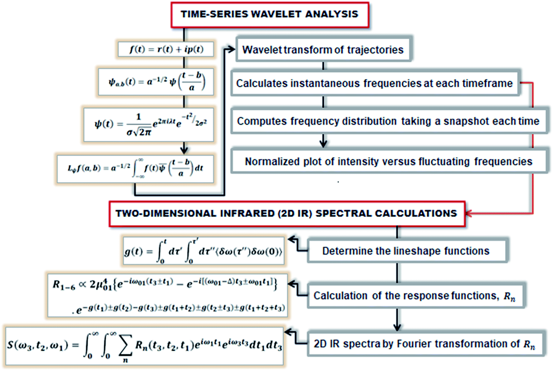
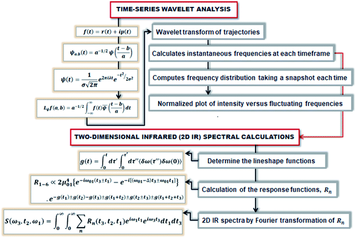
First principles molecular dynamics (FPMD) study was performed using CPMD simulation package61 employing the Car–Parrinello method.62 A deuterated system containing a single glycine and 30 water molecules was simulated in a cubic box, having a box length of 10.13 Å. Periodic boundary conditions were applied in three dimensions to eliminate the surface effects, and the electronic structure of this system was represented by the self-consistent Kohn–Sham equations63 of density functional theory64,65 within a plane wave basis. The plane wave cut off of 80 Ry was used, and we used Troullier–Martins atomic pseudopotentials66 to treat core electrons. BLYP67,68 functional with dispersion correction69 (BLYP-D2) was used. Previous reports on water simulations exhibited a dramatic rise in density with the addition of dispersion corrections to the density functionals, but the choice of BLYP-D2 density functional reported a density value close to the liquid density of water.70 The calculation of oxygen–oxygen radial distribution function (RDF) using the same functional reflected perfect tetrahedral hydrogen bond associations.71 The formamide–water system simulated using BLYP-D2 density functional adopting the same protocol provided an good agreement between the theoretical calculations and the experimental results.72 Hence, we were motivated to account for the dispersion forces in our simulations with BLYP-D2 density functional. A time step of 5 a.u. was used for the simulations with a fictitious mass of 700 a.u. to describe the electronic degrees of freedom at 300 K. We carried out wavelet analysis73,74 of trajectories obtained from the first principles molecular dynamics simulations to generate the time-dependent instantaneous frequencies of the probe OD groups. The probe encounters different environments, and owing to varied interactions, we see the change in OD vibrational stretch frequency with time, called the phenomena of spectral diffusion. Fourier analysis generates frequencies from time-dependent signals. However, the frequency representations do not establish time-frequency relationships or impart spectral information relative to time. The time-frequency dependence introduced the concept of instantaneous frequencies represented by the following functional form f(t) = a(t)eiØt and the derivative of the phase function Ø defines frequency. Time-series wavelet method73,74 determines the instantaneous frequency at each time step incorporating a time localization parameter. Wavelet analysis is an appropriate method of calculating the frequencies fluctuating with time and it provides a better time localization and spectral information. A complex function of mother wavelet f(t), is expressed as a combination of time-dependent real and imaginary termswhere r(t) is the real part representing instantaneous fluctuations of the OD bond, and ip(t) representing momentum in the above equation. The complex equation is a function of two variables a and b, which expresses translations and dilations in terms of the mother wavelet:| |
 | (2) |
ψa,b(t) has compact support or decays to 0 rapidly for at t → ±∞. The wavelet transform of f(t), gives the coefficients a and b. The coefficients of the expansion are given by the wavelet transform of the function:| |
 | (3) |
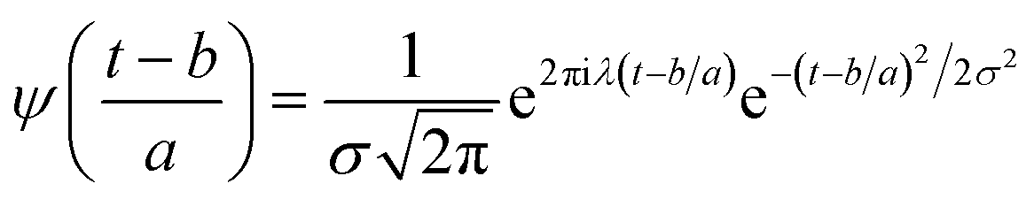
In the above equation, a > 0, b is a real term and ![[small psi, Greek, macron]](https://www.rsc.org/images/entities/i_char_e0d9.gif) represents the Fourier transform of ψ. Wavelet transform considers a time-frequency representation f; the parameter b shifts the wavelets so as to store the local information of f in Lψf(a,b) at time t = b. Lψf(a,b) depicts the frequency of f over the time interval t = b. Wavelet theorem expresses itself in terms of two functions frequency variable a (also known as scale factor) and time-variable b. The frequency variations are regulated by the dilation parameter a. The wavelet ψa,b shrinks for |a| ≪ 1, mostly in the higher frequency range and for |a| ≫ 1, ψa,b dilates with the frequency content in the low frequency range. After wavelet analysis at each time window t = b, we get the frequency of the OD mode from the inverse of scale factor a. The scale value a governs the width of the time window. At high frequency, the small value of a automatically narrows the time window, and the time window widens at a low frequency due to the large a value. Morlet–Grossman wavelet75 is used for analysis
represents the Fourier transform of ψ. Wavelet transform considers a time-frequency representation f; the parameter b shifts the wavelets so as to store the local information of f in Lψf(a,b) at time t = b. Lψf(a,b) depicts the frequency of f over the time interval t = b. Wavelet theorem expresses itself in terms of two functions frequency variable a (also known as scale factor) and time-variable b. The frequency variations are regulated by the dilation parameter a. The wavelet ψa,b shrinks for |a| ≪ 1, mostly in the higher frequency range and for |a| ≫ 1, ψa,b dilates with the frequency content in the low frequency range. After wavelet analysis at each time window t = b, we get the frequency of the OD mode from the inverse of scale factor a. The scale value a governs the width of the time window. At high frequency, the small value of a automatically narrows the time window, and the time window widens at a low frequency due to the large a value. Morlet–Grossman wavelet75 is used for analysis
| |
 | (4) |
Expressing eqn (4) in terms of 
| |
 | (5) |
Substituting  in eqn (2),
| |
 | (6) |
ψ must be real and should satisfy the admissible condition,
, and
λ = 1 and
σ = 2 are the values for constants. These parameters are adjusted to get better resolution in the calculated frequencies. The snapshots of trajectory frames undergo Fourier transformation
76 of time-domain data to generate frequencies. Wavelet code runs through the entire trajectory and computes the frequency
77,78 of all OD modes.
The linear spectroscopy gives a time-averaged broad vibrational absorption spectrum owing to the variety of surrounding local environments. Two-dimensional infrared (2D-IR) vibrational echo spectroscopy79,80 is a useful tool to track the molecular interactions occurring at sub-picosecond to picosecond timescales in the fastest chemical exchange reactions, solute/solvent interactions and solution dynamics,81–83 water dynamics,84,85 and hydrogen network evolution.86 For accessing the dynamics in the aqueous solvation shells, a vibrational chromophore known as the probe entity is chosen. Here, OD vibrational stretch is the probe of interest. Probes respond to the changes in the local environment by interacting with them, resulting in its vibrational stretch frequency changes referred to as the phenomena of spectral diffusion.87 Spectroscopic techniques like IR, NMR can track the chemical processes if timescales are slow. However, ultrafast vibrational spectroscopy can interrogate the molecular structure and ultrafast intermolecular motions. The time-dependent frequencies of the OD modes obtained from the time-series wavelet analysis73,74 were used for the calculation of non-linear vibrational spectral features of the water molecules in the solvation shell of ammonium and carboxylate groups of glycine presented in Fig. 5. We employed second-order cumulant approximation of the response function88–90 in our calculation of the 2D-IR spectrum. In this approximation, it is assumed that the fluctuating dynamics describe a Gaussian process and is valid for observing the peak shift. However, in strongly hydrogen-bonded systems like liquid water, non-Condon line shape is more realistic as it takes into account non-Gaussian frequency fluctuations and environmental impacts on the transition dipole (non-Condon effects).88
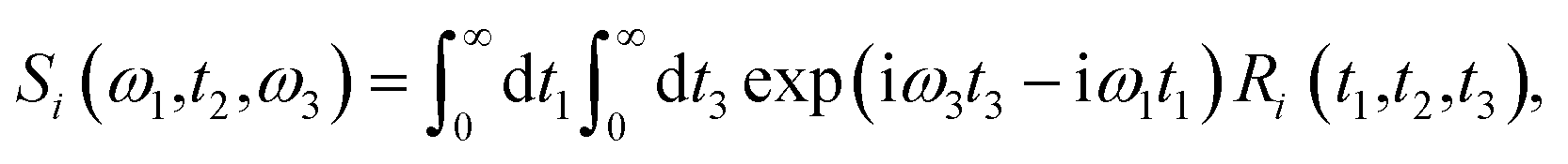
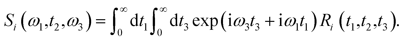
Theoretical calculations of the 2D-IR spectroscopic observables involve response function formulation.88,90 Three ultrashort IR pulses with wave vectors k1, k2, and k3 interacts with three input electric fields E1, E2, and E3 to produce an echo signal Esig. Previously reported literature has the details of the 2D-IR experimental setup79,85 and derivations of the mathematical formulae.88–90 Ignoring, the excited state and rotational lifetime effects, the equations for response functions in second-order cumulant approximation is given by
| |
R1(t3,t2,t1) = R2(t3,t2,t1) = μ104![[thin space (1/6-em)]](https://www.rsc.org/images/entities/char_2009.gif) exp(−i〈ω10〉t3 + i〈ω10〉t1) × exp(−g1(t1) + g1(t2) − g1(t3) − g1(t2 + t1) − g1(t2 + t3) + g1(t1 + t2 + t3)), exp(−i〈ω10〉t3 + i〈ω10〉t1) × exp(−g1(t1) + g1(t2) − g1(t3) − g1(t2 + t1) − g1(t2 + t3) + g1(t1 + t2 + t3)),
| (7) |
| | |
R3(t3,t2,t1) = −μ104κ2exp(iΔt3) × exp(−i〈ω21〉t3 + i〈ω10〉t1) × exp(−g1(t1) + g2(t2) − g3(t3) − g2(t2 + t1) − g2(t2 + t3) + g2(t1 + t2 + t3)),
| (8) |
| | |
R4(t3,t2,t1) = R5(t3,t2,t1) = μ104exp(−i〈ω10〉t3 − i〈ω10〉t1) × exp(−g1(t1) − g1(t2) − g1(t3) + g1(t2 + t1) + g1(t2 + t3) − g1(t1 + t2 + t3)),
| (9) |
| | |
R6(t3,t2,t1) = −μ104κ2exp(iΔt3) × exp(−i〈ω21〉t3 − i〈ω10〉t1) × exp(−g1(t1) − g2(t2) − g3(t3) + g2(t2 + t1 ) + g2(t2 + t3) − g2(t1 + t2 + t3)).
| (10) |
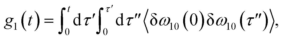
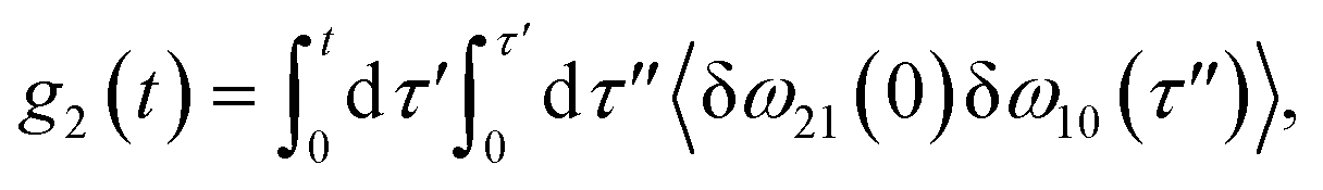
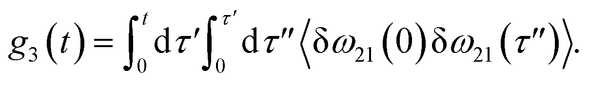
The time delay between the first and second pulses is referred to as t1, between second and third pulses as t2, t2 = Tw(waiting time), and the time after the third pulse as t3. g1(t), g2(t) and g3(t) are the time correlations of the fluctuating transition frequencies given by the following expressions
| |
 | (11) |
| |
 | (12) |
| |
 | (13) |
where
Δ = 〈
ω21〉 − 〈
ω10〉 and
κ is equal to
μ21/
μ10.
μ10 and
μ21 represent the transition dipole moment corresponding to 0–1 and 1–2 transitions.
ω10 and
ω21 correspond to the vibrational frequencies of the mode in the ground and excited state.
Δ value gives the measure of anharmonicity. 2D IR spectrum is obtained by Fourier transformation of the response functions along the two frequency axes in terms of waiting time (
t2 =
Tw) expressed as follows
88–90| |
 | (14) |
where,
| |
 | (15) |
for
i = 1 to 3 and
| |
 | (16) |
for
i = 4 to 6, respectively.
At initial Tw, the final frequencies are found to be similar to the initial frequencies. The frequency correlation initiates the phenomena of spectral diffusion, and the 2D-IR line shape is seen elongated along the diagonal axis. At higher Tw, the final frequencies are different from the initial value, and the frequencies decorrelate with time. Thus, with time more spectral diffusion occurs, resulting in frequency decorrelation quantified by a symmetrical 2D-IR line shape.91 Fig. 3 depicts the diagrammatic scheme of frequency calculations based on wavelet theory and the mathematical formulation of the 2D IR spectrum from the calculated time-dependent fluctuating frequencies.
3. Results and discussion
3.1. Structural aspects of the solvation regime in aqueous glycine
To understand the structure in aqueous glycine solution, we calculated the pair correlation function or radial distribution function (RDF). The RDF, g(r), determines the atomic density at a certain distance away from the reference molecule in a system of molecules92,93 given by| |
 | (17) |
where ri and rj depict the magnitude of the position vectors of the ith and jth particle. RDF was calculated by constructing histograms,93 inserting atom pair distances in each trajectory timeframe, and it provides a detailed description of the condensed phase liquid structure.
In the RDF graph shown in Fig. 1, the location of the first peak minimum is taken as the distance cut-off for defining the solvation boundary of the corresponding intermolecular atomic pair in the glycine solution. We computed intermolecular RDFs between the atoms of glycine molecule and the oxygen (OW) or deuterium (DW) atoms of the neighboring water molecules, i.e., the radial distribution of N–OW, DN–OW, DC–OW, OC–OW, and OC–DW pairs to create a solvation shell demarcation94 from the bulk around amine nitrogen, methylene groups and carboxylic oxygen in aqueous glycine. DN, DC, and OC represent the deuterium atoms attached to nitrogen, deuterium atoms of the methylene group, and two oxygen atoms adjacent to the carboxylic carbon, respectively. The corresponding number integrals (NIs) are also presented together with the RDFs in Fig. 1 by the dashed lines. The number integral NI(r) is expressed by the equation
| |
 | (18) |
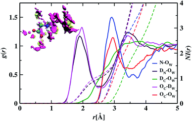 |
| | Fig. 1 In the glycine–water system, the solid lines blue, maroon, green, magenta, and red represent the radial distribution functions (RDFs) for N–OW, DN–OW, DC–OW, OC–DW, and OC–OW pairs, respectively and the corresponding number integrals (NI) are shown with dashed lines. The SDF of oxygen and deuterium atoms are shown with magenta and yellow colored isosurfaces (isovalue = 78), respectively, in the upper part (inset figure). | |
The value of the number integral at the first peak minimum of RDF estimates the coordination number or hydrogen bond number depending on the types of atoms involved. Analysis of the RDF provides the structural details in solvated zwitterionic glycine. The first peak maximum, minimum, and corresponding values of the number integral of the N–OW RDF pair are 2.81, 3.48 Å, and 3.5 in accordance with the N–OW RDF data given by the ab initio molecular dynamics (AIMD) study of one glycine and 30 water molecules.8,95 Neutron diffraction experiments96 and Car–Parrinello8 method reported 3 to 4 solvation water molecules around the ammonium group in glycine. The latter AIMD simulation8 slightly overestimates the solvation number to four, but the number is reduced to three when the HN–OW interactions are eliminated. A slight hump in noticed in g(N–OW) at the minimum due to the interactions from the extra solvent water (NI = 3.5) at its vicinity. The first peak minimum of DN–OW RDF at 2.44 Å serves as the hydrogen bond cut-off criteria inside the aminic nitrogen solvation shell in the glycine system. Three water molecules, found in the first solvation sphere around the ammonium group, match with the previous CPMD study of glycine intramolecular proton transfer in water.8 This seems to be quiet interesting as we can say that each hydrogen bond donor site in the amine group is hydrogen-bonded to one of its nearest neighboring oxygen atom of water displaying strong hydrogen bond interactions. A second peak is seen in the N–OW radial distribution function plot extending to a minimum at 4.3 Å, and the second solvation shell is not well defined because of its shallowness compared to the first peak minimum. Thus, the second hydration layer around aminic nitrogen lies undefined as in preceding reports.95 The RDF of DC–OW pair around methylene functionality reflects very weak interaction with the nearby water as there is no sharp peak maximum. The solvation boundary is not well-defined with minimum extending up to 4.3 Å due to the water-repelling nature of CD2 moiety that inhibits the approach of water molecules. Moving the attention towards the carboxylates, we calculated OC–OW RDF, and the first peak maximum appears at 2.85 Å matching with the previously reported values,97,98 and the first solvation shell is at a distance of 3.30 Å, (at the first peak minimum) around carboxylic oxygen of glycine. To count the number of water molecules hydrogen-bonded to OC in the COO solvation, we calculated the pair correlation function of OC–DW, the first peak minimum is observed at 2.52 Å. Within this distance, the water hydrogens are hydrogen-bonded to the carboxylic oxygen. The number integral at the first minimum is found to be 4.3 yielding one water molecule with two deuterium atoms near each OC. On average, a total of 4.7 number of hydrogen bonds were reported within water and carboxylate oxygen atoms.8 However, both the values were found to be smaller than the hydration numbers 5.3 and 7 predicted by simulations using empirical force field99 and OPLS force fields100 respectively. Classical molecular dynamics study101 with AMBER ff03 force field showed the first peaks in RDFs of OC–OW, HN–OW, and N–OW pairs at 2.71, 2.05, and 2.95 Å, respectively, were in good agreement with various organic crystals.102 The hydration numbers reported by the study of glycine/water mixtures101 in crystal/solution environments around amino and carboxylic groups were 2.97 and 5.38, respectively. Neutron diffraction measurements48 with isotopic substitution showed 3 water molecules around the amino group on an average and 4 to 5.5 water molecules representing more hydrophilicity around the carboxyl group.
We visualized the probability of finding the oxygen and deuterium atoms around the glycine molecule in a three-dimensional space by calculating the spatial distribution function (SDF). An isosurface plot shown at the inset of Fig. 1, having isovalue of 78, was used to represent the oxygen and deuterium atoms of water molecules around glycine. The concept of isosurface103 comes from contour lines passing through the areas with the same probability in topographic maps. SDF data of water molecules around ND3, CD2, and COO groups in aqueous zwitterionic glycine reveal that the atomic oxygen distribution is denser than that of hydrogen atoms around all three sites. The 3D figure representing the spatial distribution of water molecules around two hydrophilic zones, the amine nitrogen, and carboxylic oxygen enables us to determine water's structural arrangement around hydrophilic groups and distinguish it from the distribution pattern of the water molecules around hydrophobic methylene. In the SDF figure, we find a small fraction of water molecules around the apolar methylene group; this justifies the water-repelling nature of hydrophobes. However, there is a dense distribution of water molecules around water-loving amine nitrogen and carboxylic oxygen sites in glycine. A close view of the atom cloud density at the COO group in solvated glycine reveals the non-uniform distribution of water molecules around the two carboxylic oxygen atoms (OC), which behave little differently. Moreover, splitting of the hydrated HDO infrared band76 and ab initio molecular dynamics simulations95 revealed carboxylate anion underwent nonequivalent interaction with hydrating water via two oxygen atoms.
In the aqueous solution, we find glycine in the zwitterion state possesses two hydrophilic hydrogen bonding sites around aminic nitrogen and carboxylic oxygen. In order to gain deep insight into the hydrogen bonding patterns, we calculated the combined distribution function (CDF), as shown in Fig. 2. The figure presents the combined plot of distance [R in pm] along the X-axis versus the angular distribution of the hydrogen bond angle formed by two vectors represented by angle [θ in degrees] along the Y-axis. The intercalated models in the top and bottom panel of Fig. 2 provide the information regarding the distance and H-bond angle considered here. SDF and CDF were computed using the TRAVIS software package.103 In the contour plot shown in the upper panel, we find the CDF in aminic nitrogen solvation shell, considering N–OW distance and the angle formed by the bond vectors N–DN and DN–OW. The most probable angle is found to be around 15° at a distance of 300 pm, and the dark-colored angular distribution ranges from 0° to 23° within the N–OW distance of 280 to 320 pm. Light green colored contour is visible along 90° to 135° in the same N–OW distance range, but the probability of finding it is very less. In Fig. 2(b), the hydrophilic carboxylic group in glycine, the gnuplot exhibits CDF of OC–OW distance, and the angle formed by the hydrogen bond between DW of water and acceptor site OC, the OW–DW⋯OC bond angle. In this case, the darker color depicts the most probable OC–OW distance at 300 pm, and the angular distribution lies along 165°. Along distance from 280 to 320 pm, the angular distribution stretches, and the OC–OW distance 320 pm marks the first minimum (3.30 Å) of the OC–OW RDF peak. We also find a light green patch along 45° to 75°, but it is a region that is less probable and not so well defined.
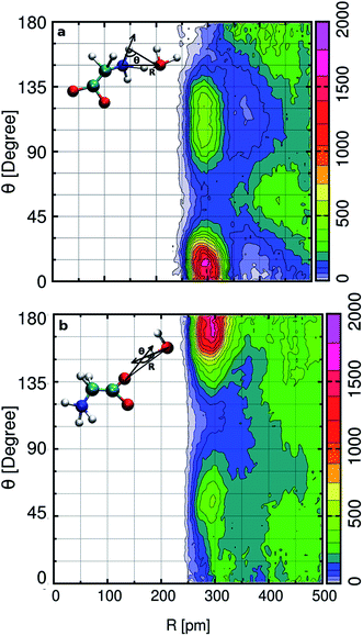 |
| | Fig. 2 In the top panel (a) the x-axis represents N–OW distance (in pm), and the y-axis represents the hydrogen bond cut-off angle between two bond vectors N–DN and DN–OW. The bottom panel (b) represents the CDF of OC–OW distance and the hydrogen bond angle that originates from OW–DW and OC–DW bond vectors. | |
3.2. Distribution of O–D stretch frequency inside hydrophilic and hydrophobic hydration shell of glycine
The analysis of RDF, SDF, and CDF depicts the structural arrangement and behavior of the different types of water molecules around glycine. The distribution of water molecules in glycine solvation seems to be heterogeneous, but this topic has not been explored in great detail so far. Therefore, we classify the solvation shell of aqueous zwitterionic glycine into three sections to understand the non-uniform solvation of water molecules. We categorize these as two hydrophilic regions, one around amine nitrogen and the other carboxylic oxygen, and hydrophobic methylene based on the hydrogen bonding motifs. The RDF data already shows the presence of strong hydrogen bonding environments around water-loving –ND3 (DN⋯OW) and –COO (OC⋯DW) groups and the weakly interacting water molecules around hydrophobic methylene.
A division is made in between the solvation shell and bulk104 based on RDF calculations, and the solvation boundary was defined around aminic nitrogen taking N–OW RDF peak minimum at 3.48 Å, and the criteria for hydrogen-bonded water molecules in this nitrogen solvation was taken from DN–OW minimum at 2.44 Å. In a similar way, peak minima of radial distribution, OC–OW at 3.30 Å, and OC–DW at 2.52 Å were taken as the solvation shell condition and cut-off distance94 within which water acts as the proton donor to participate in hydrogen bonding with the C-terminal oxygen in –COO. A sharp peak is absent in DC–OW RDF, and the solvation shell around methylene is not pronounced, but still, the distance 4.3 Å marks the limit of the solvation zone of water molecules around –CD2. Bulk water refers to those solvent molecules that are outside the amine, carboxylic, and methylene hydration sphere.
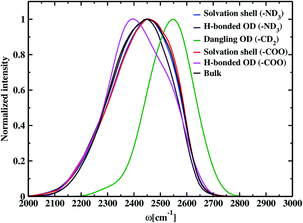
The time-dependent vibrational stretch frequencies of all the OD modes were calculated using the wavelet method of Arevalo and Wiggins74 and was found to be 2416 cm−1. Raman spectrum recorded a bifurcated D2O stretching region with peaks at 2190 and 2390 cm−1 and revealed the former band had more intensity than the later with the increase in the concentration of dissolved molecules.105 IR spectra of deuterated glycine derivatives in low-temperature argon matrix exhibited spectral features in three most stable glycine conformers for the first time and assigned the frequencies to the stretching and bending vibrations.106 These matrix-isolated IR spectra of the deuterated glycine portrayed a spectral signature at 2399 cm−1 for the OD stretch, and the peak characteristics were dependent on the conformation of glycine. DFT calculations, carried out using the B3LYP density functional and aug-cc-pVDZ basis set, reported the O–D stretch band at 2411 cm−1 and helped to identify the IR spectral characteristics of the glycine conformers in the experiment. Our calculated value of the average frequency of all the OD bonds in deuterated glycine ∼2416 cm−1 is close to the computed OD stretch frequency 2411 cm−1. Solute-affected HDO spectra and DFT calculations using the polarizable continuum model showed that splitting of HDO band was due to the asymmetric distribution of water molecules around ammonium and carboxylate groups of glycine.107 It is difficult to determine the frequencies inside each of the hydration regions and outside it by applying the solvation shell conditions experimentally,108 but the computational tools enable solvation zone wise calculation of the normalized frequency distribution, which is displayed in Fig. 4. Inside the N–OW solvation shell, the vibrational stretch frequency is 2425 cm−1. Inside aminic nitrogen solvation shell, OD modes that form DN⋯OW hydrogen bond has an average frequency of 2418 cm−1, exhibiting a bathochromic shift of 7 cm−1. We also observe a higher value of the average frequency 2550 cm−1 around methylene of the amino acid; therefore, we predict the dominant contribution of non-hydrogen bonded water molecules or the free OD modes due to weak interaction of the methylene hydrogen and nearest neighboring oxygen leading to hydrophobic hydration in glycine. A characteristic sharp peak at ∼2580 cm−1 in the vibrational power spectrum marked the presence of dangling OD modes together with the hydrogen-bonded OD modes in water–carbon tetrachloride (liquid–liquid) interface.109 Stretch frequency distribution in aqueous ionic solutions like carbonate,110 and phosphate ion111 showed a broad spectral feature lying in the range 2500–2700 cm−1 representing dangling OD groups. Inside the solvation regime of carboxylic oxygen, the average frequency is 2423 cm−1, and the solvation shell O–D stretch frequency of aminic nitrogen is 2425 cm−1. Similarly, in the aqueous solution of N-methyl acetamide, the average stretch frequency of the OD modes using BLYP and BLYP-D3 density functionals were reported to be 2459 and 2465 cm−1, respectively, inside amine nitrogen solvation shell; moreover, 2341 and 2346 cm−1, respectively, inside carbonyl oxygen hydration shell.112 Till now, the observed frequency shifts are within ±7 cm−1 for hydrophilic solvation and ∼25 cm−1 around hydrophobic –CD2 due to the existence of dangling OD modes of water near it. Carboxylate–water hydrogen bonds with average frequency 2397 cm−1 are found to be stronger than amine–water hydrogen bonds having a value of 2418 cm−1. The previous study showed that stronger hydrogen bonds were formed by the water molecules, which interact with the carboxylate group than with the hydrogens of the amine group of glycine and its N-methylated derivatives.76 Bulk OD modes with frequency 2410 cm−1 are in agreement with the computed average O–D stretch frequency value (∼2380 cm−1) of heavy water,78 and the experiments reported vibrational stretch of the OD band centered at ∼2500 cm−1.113 The discrepancies are a result of the difference in electronic structure calculations with different density functionals, electronic fictitious mass, and finite basis set cut-offs.114,115 Comparing the bulk average O–D stretch frequency (∼2410 cm−1) with the average frequency of OD modes hydrogen-bonded to carboxylate (∼2397 cm−1), and ammonium (∼2418 cm−1); we observe that the OD groups hydrogen-bonded to carboxylate are red-shifted with respect to the water molecules hydrogen-bonded to other water at bulk, and the hydrogen-bonded OD in amine solvation is slightly blue-shifted relative to bulk. First principles molecular dynamics simulations of aqueous formamide solvation revealed carbonyl–water hydrogen bonds are stronger than hydrogen-bonded water molecules at bulk, and amine–water hydrogen bonds are weaker than bulk based on the frequency shifts.116 The trend observed in the glycine solution indicates the correlation between frequency and hydrogen bond strength matching the formamide–water system. In aqueous methylamine, a blue shift of 30 cm−1 was reported ongoing from bulk towards amine hydration shell.104 The OD modes within the solvation shell cut-off in amine hydration (2425 cm−1) show a similar 15 cm−1 frequency shift corresponding to the bulk OD stretch (2410 cm−1) in glycine. In glycine–water system, bulk water molecules exhibit a red shift in the average vibrational stretch frequency as compared to the carboxylate hydration shell and this shift is comparable to the 34 cm−1 shift observed ongoing from the carbonyl oxygen solvation towards bulk in aqueous acetone.117
 |
| | Fig. 3 The schematic represents the method of computing the 2D IR spectrum from the time-dependent frequencies obtained from the wavelet-based frequency calculations. | |
 |
| | Fig. 4 Normalized distribution of O–D stretch frequencies in the solvation shell of amine nitrogen is shown by the blue line. The maroon line represents the stretch frequencies of hydrogen-bonded OD modes inside the nitrogen hydration shell. Non-hydrogen bonded OD modes, i.e., the distribution of modes in the dangling state around hydrophobic methylene, are shown by the green line. Inside the solvation shell of carboxylic oxygen in glycine, the distribution of all OD modes and hydrogen-bonded OD modes are represented by red and magenta lines, respectively. The black line represents the bulk OD modes. | |
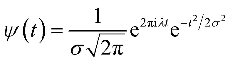
3.3. Ultrafast non-linear vibrational spectroscopy
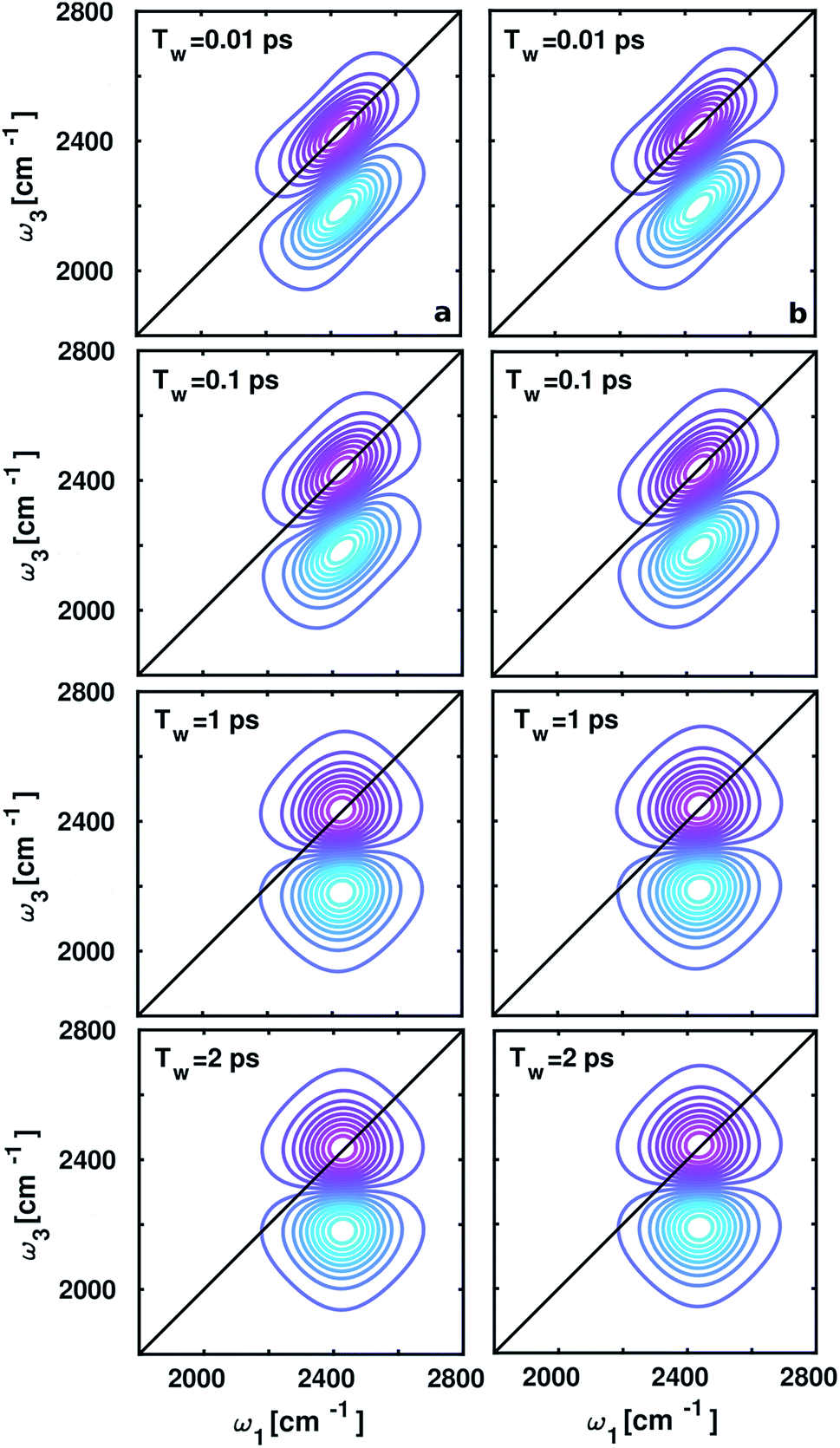
The spectral changes observed in the computed 2D-IR spectra around ammonium and carboxylate groups at different waiting times (Tw) 0.01, 0.1, 1, and 2 ps shown in Fig. 5, quantify vibrational spectral diffusion of OD modes of water molecules occurring at each timescale. The 2D-IR peak shapes are found to be similar at each Tw due to dipolar interactions between positively charged ND3+ and negatively charged COO− in aqueous zwitterionic glycine. The peak on the ω1–ω3 diagonal originates from stimulated emission and ground-state bleach from ν = 0 → 1 energy levels, and the off-diagonal peak represents vibrational excited state absorption for ν = 1 → 2 transition, shifted by anharmonicity to a lower wavenumber. In the 2D-IR contour plot around the carboxylate group, the diagonal line width of the lobes is slightly broad as compared to the ammonium; this trend matches with the full width at half-maximum (fwhm) of the O–D stretch frequency distribution inside the solvation shells in glycine.
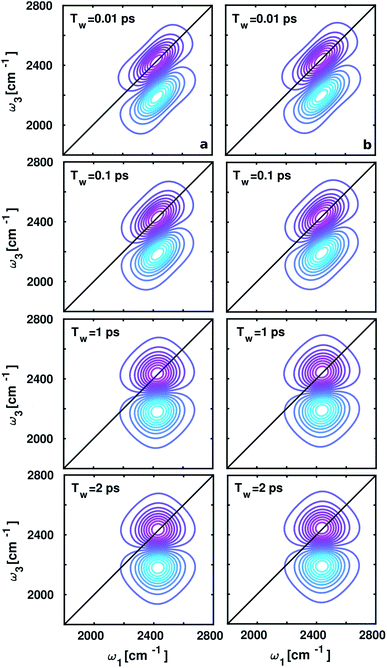 |
| | Fig. 5 2D IR spectroscopy of the OD stretch modes at four different time delays (Tw) to monitor the phenomena of spectral diffusion. Left panel (a) represents the 2D IR spectra of the solvation shell water molecules around the ammonium group, and the spectral features in the carboxylate hydration shell are shown in the right panel (b). | |
3.4. Frequency fluctuations due to environmental variations and the hydrogen bond and dangling dynamics
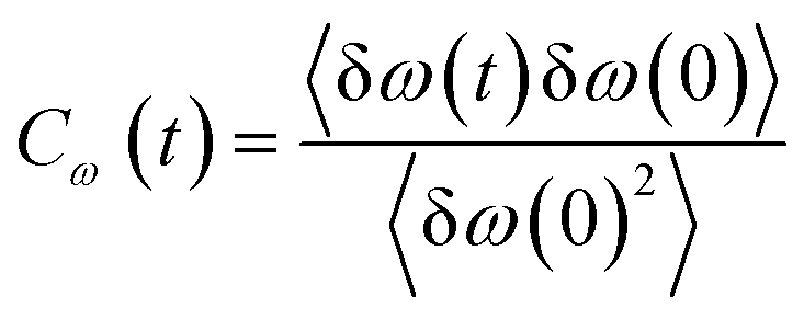
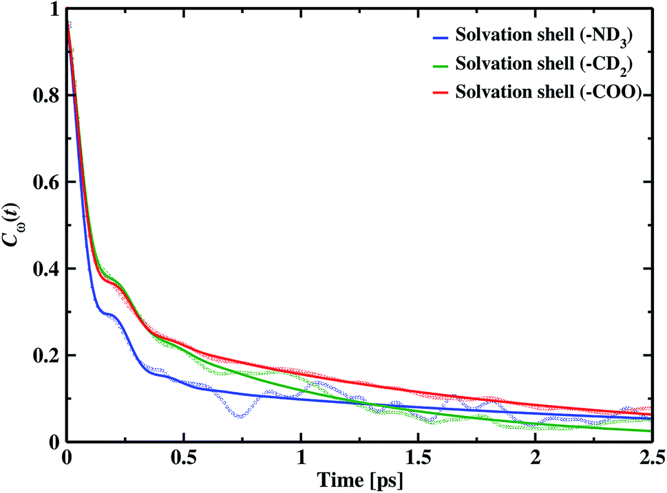
Frequency changes owing to the differences in the surrounding environment around the vibrational chromophore of interest are reported here considering O–D mode as the probe. As the probe molecule interacts with the environmental alterations, its frequency changes. Thus, frequency fluctuations serve as a reporter of the system dynamics78 and can be computed using the following relation| |
 | (19) |
where Cω(t) is the frequency–frequency time correlation function calculated by averaging over all OD bonds of interest, δω(t) is the fluctuation obtained by subtracting the average value from instantaneous frequency. The decay of fluctuations in frequency correlation is shown in Fig. 6. Table 1 displays the timescales and weight parameters obtained by fitting the decay curve with the damped oscillatory fitting function118,119| | |
f(t) = a0cosωste−t/τ0 + a1e−t/τ1 + (1 − a0 − a1)e−t/τ2
| (20) |
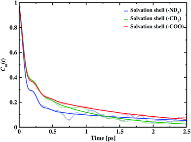 |
| | Fig. 6 The blue line shows the frequency–frequency time correlation decay of the amine nitrogen solvation shell OD modes. The frequency correlation in the hydration of the methyl group is shown by the green line, and the solvation shell of carboxylic oxygen is shown by the red line. The hazy lines show raw data, and the solid lines give the fitted data, fit by the damped oscillatory tri-exponential fitting function. | |
Table 1 The frequency–frequency correlation function parameters are listed below. The timescales and the frequencies are in ps and cm−1 units respectively
| Cω(t) |
τ0 |
τ1 |
τ2 |
ωs |
a0 |
a1 |
| Solvation shell (–ND3) |
0.08 |
0.98 |
5.10 |
95.32 |
0.52 |
0.31 |
| Solvation shell (–CD2) |
0.09 |
0.58 |
4.49 |
98.26 |
0.55 |
0.40 |
| Solvation shell (–COO) |
0.09 |
2.07 |
5.23 |
99.84 |
0.46 |
0.39 |
A faster component appears in the range of 80–90 fs timescale due to the underdamped motions of intact hydrogen bonds. We also find two other time constants, the intermediate time constant and the slowest timescale extending to a few ps. The intermediate timescales are in the range 0.5 to 2.0 ps, and the longest timespan corresponds to 4.49 ps around hydrophobic methylene and approximately 5.0 ps in hydrophilic solvation shells.
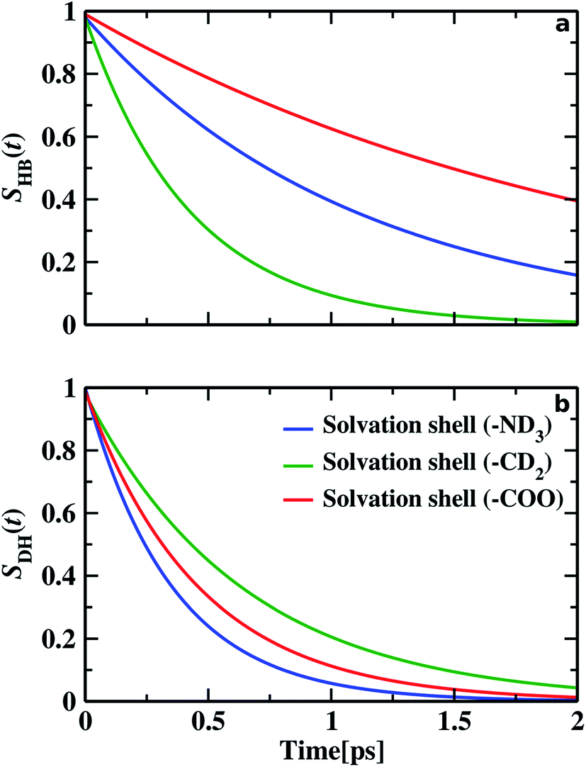
We find different types of hydrogen bonding interactions around glycine. Previously covalent-like hydrogen bonds had been confirmed by penetrating molecular-orbitals of glycine–water clusters.54 We also calculated the continuous hydrogen bond time correlation function, SHB(t).120–125 The auto-correlation function is defined with the help of the population correlation function approach115,126
| |
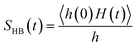 | (21) |
Here, we compute the probability of hydrogen bond to remain continuously hydrogen-bonded from time
t = 0 up to
t =
t.
h(
t) and
H(
t) refer to the bond parameter.
h(
t) = 1, when a particular pair of glycine molecules remain hydrogen-bonded at time
t and zero if the hydrogen bond is broken. Similarly,
H(
t) = 1 when all hydrogen bonds fulfill the geometric criterion and remain in the bonded state at all times. In computer simulations, liquid water is modeled as a system consisting of
N water molecules,
r(
t) denotes the position of all atoms at time
t, and
h represents the average of
h[
r(
t)].
120,127 In the definition of the time-dependent hydrogen bond fluctuations, the denominator
h in
eqn (21) is presented as the normalization factor
h(0)
2 in other studies.
87,117 Integrating
SHB(
t), we compute the hydrogen bond lifetime (
τHB).
78 In the apolar hydrophobic solvation shell of methylene of glycine, we explore the predominant presence of dangling OD.
SDH(
t)
128 represent the probability of a dangling mode to remain non-hydrogen bonded in the dangling state.
τDH gives the time period, the OD mode of water remains dangling. Time dependence of hydrogen bonds and dangling OD modes of water molecules in each of the solvation shell are shown in
Fig. 7.
SHB(
t) yields hydrogen bond lifetime (
τHB) for amine–water and carbonyl–water as 1.09 and 2.17 ps, respectively. It is seen that the lifetime of O
C⋯D
W hydrogen bond is twice that of D
N⋯O
W hydrogen bond. This fact verifies the results of our frequency distribution, where the carboxyl–water hydrogen bond is found to be stronger, reflected by the double lifespan of hydrogen bond than the hydrogen bond in amine–water. Comparing the lifespan of hydrogen bonds in hydrophobic methylene solvation, 0.42 ps, the average dangling lifetime of non-hydrogen bonded OD is found to be 0.64 ps. This proves the predominance of free water molecules around the hydrophobic methylene group. The dangling lifetime of OD modes inside hydrophilic solvation is found to be 0.35 ps for aminic nitrogen and 0.46 ps for the carboxylic oxygen hydration sphere. Therefore, near hydrophilic sites, we find the water molecules are forming D
N⋯O
W and O
C⋯D
W hydrogen bonds.
 |
| | Fig. 7 The upper panel (a) represents the continuous hydrogen bond correlation function, and the lower panel (b) displays the time-dependent decay of the continuous dangling OD probability function. The blue, green, and red lines represent the dynamics of hydrogen bonds and dangling OD groups inside the solvation shell of amine nitrogen, methylene, and carboxylic oxygen, respectively. | |
As time pass over the hydrogen bonds are broken, then either of the two things may happen: water molecules with the broken hydrogen bond stay inside the solvation shell but remain non-hydrogen bonded with the glycine molecule before it again reforms the hydrogen bond or the water molecules leave the solvation shell and diffuses away. We calculated the residence time correlation function SR(t). By fitting the decay curve with a bi-exponential equation, we get the residence time (τR). Residence time measures the lifetime of water molecules inside the solvation shell. τR of water molecules inside N–OW solvation shell, around methylene group and carboxylic oxygen solvation shell in glycine, are 5.18, 4.22, and 5.38 ps, respectively. We examine the similarity between the timescales of the frequency–frequency correlation function and the dynamics of hydrogen bonds and dangling OD modes. Along with the hydrophilic sites, the hydrogen bond lifetime, 1.09 ps (for HN⋯OW), and 2.17 ps (OC⋯OW) are comparable to the faster component of picosecond timescale of the decay of frequency–frequency time correlation function. For hydrophobic solvation, the dangling lifetime 0.64 ps is found similar to the intermediate component of frequency fluctuations (0.58 ps), validating the fact that the dangling water molecules are responsible for the frequency alterations in hydrophobes. The longest time constant of frequency correlation corresponds to the escape dynamics of water molecules from the solvation shell, also known as the residence dynamics.
4. Conclusions
Glycine is one of the simplest biologically relevant neutral amino acids, which is stabilized by the formation of zwitterion129 in aqueous solution. Many structural studies on the most stable glycine conformer exist,42,44,130,131 but the dynamical aspects and ultrafast non-linear spectroscopy of deuterated hydroxyl groups of water molecules in the solvation shell of glycine remain unexplored. Here, we present dynamics and 2D-IR spectroscopy of water molecules of the solvation shell of glycine using first principles molecular dynamics simulations by tracing the water molecules by their distinctive behavior towards heterogeneous solvation facilitated primarily by two functional groups of amino acid: hydrophobic and hydrophilic. We performed structural calculations like radial distribution function (RDF) to understand the solvation shell demarcation.94,104 For aminic nitrogen and carboxylic oxygen, the solvation shell criteria are N–OW distance less than 3.48 Å and OC–OW distance less than 3.30 Å, respectively. For methylene, the DC–OW RDF peak minimum extends up to 4.2 Å. It limits the hydration shell as there is no sharp and well-defined peak because of poor interaction with the apolar hydrophobe methylene group. An isosurface plot of atomic cloud density reveals the dense population of oxygen atoms around glycine. A close view of SDF shows the uneven distribution, sparsely populated water molecules around water-hating methylene, and dense distribution along with hydrophilic sites. A contour plot of distance versus hydrogen bond angle re-verifies the RDF data.
The wavelet method74 was used to compute the instantaneous frequency of the stretching mode of water molecules in various environments. The distribution of normalized intensity versus wavenumber was plotted for each of the solvation zones, and it was found that the average frequency around hydrophobic methylene is blue-shifted to 2550 cm−1 than the hydrophilic solvation sites where the average frequency lie around 2424 cm−1. However, applying the geometric criteria of the formation of hydrogen bonds, we find carboxylate–water hydrogen bonds are stronger than amine–water ones, and water molecules with free (or dangling) OD groups are found around hydrophobic methylene. To report the dynamics prevalent in glycine, the effect of environmental changes on the OD vibrational stretch was monitored from the frequency fluctuations with time. In this present study, the OD vibrational stretch serves as the local probe for 2D-IR to determine the ultrafast structure and dynamics in aqueous solvation shells in glycine. The second-order cumulant approximation was applied to generate the 2D-IR spectrum and expose the bonding patterns in aqueous solvation as a function of peak shift observable. A slight bathochromic shift is observed in the average OD stretch frequency distribution in the carboxylate solvation shell as compared to the hydration shell of amine nitrogen. Thus, the shape of the 2D-IR spectrum at each reported waiting time is similar around both the hydrophilic sites owing to the negligible peak shift, and the diagonal line width of the lobes are in accordance with the fwhm of the frequency distribution plot in the respective solvation shells. The broader diagonal width in the carboxylate solvation shell distinguishes the structural patterns and dynamical response within the two hydrophilic hydration sites in glycine. In the analysis of frequency-time correlation in each solvation shell, we observe three timescales: a rapid decay in femtosecond time owing to the librational motion of intact hydrogen bonds, the intermediate time constant corresponds to the lifetime of hydrogen bonds for hydrophilic functional groups and dangling lifetime for weakly interacting methylene solvation. Lastly, the slowest picosecond time constant reflects the time period the water molecules stay in the corresponding solvation shell. It is found that the lifetime of a carboxylate–water hydrogen bond is twice that of amine–water. Residence times around the hydrophobic methylene and around hydrophiles are 4.22 and ∼5.0 ps; respectively, due to the presence of free water molecules, they readily escape from the hydration shell in water-hating hydrophobes. Thus, the classification of aqueous glycine hydration shells in three solvation regimes enables us to explore both the structure and solvation shell dynamics occurring at the sub-picosecond to picosecond timescales and thereby, comment on the diversity that exists in the vicinity of aminic nitrogen, carboxylic oxygen, and methylene groups.
In this study, we investigate the response of water molecules towards the differential site-specific interactions of glycine. Structural aspects in solvated glycine had been reviewed in the past, but we emphasize the solvent dynamics existing in glycine solution. Our calculations help in unveiling the heterogeneous dynamics induced by the heterogeneity in structure facilitated by both the hydrophilic and the hydrophobic environments. Limitations of the experimental technique in analyzing the structure and the dynamics of vibrational spectral diffusion through spectroscopic measurements inside the solvation shell demanded support from the molecular modeling approach. Our method of calculation enables us to capture the differential solvent interactions with each of the hydrophilic and the hydrophobic sites inside the hydration shell of glycine. Hence, computation serves as an exquisite tool that can overcome the drawbacks of the experiments performing calculations and analyzing the structural, spectral, and dynamical properties inside the solvation shell. The numerous experimental and theoretical results, discussed here, provide structural evidence and exhibit the vibrational O–D stretch spectra of the water molecules in the vicinity of glycine. Our analysis of the vibrational spectrum agrees with the experimental measurements hinting the level of accuracy involved in our calculations. Structural calculations, such as the radial distribution functions (RDFs), demarcate the solvation boundary specific to a particular functional group. We classify the solvation shell of glycine into three regions based on the RDF data: the aminic nitrogen hydration shell, hydrophobic methylene solvation, and the solvation boundary around carboxylate. In each of the solvation regimes, we monitor the spectrum of the OD vibrational stretch band, time-dependent decay of frequency fluctuations, and spectral shifts due to the hydrogen bonded O–D modes and dangling water molecules inside the solvation shell. Ultrafast 2D IR spectroscopy is a powerful experimental technique that interrogates ultrafast molecular motions. In the current work, we employ the time-dependent frequencies obtained from the wavelet theorem and perform the 2D IR spectral calculations to distinguish between the two hydrophilic solvation shells of aminic nitrogen and carboxylic oxygen depending on the diagonal line width reflected in the 2D IR spectrum. We further quantify the strength of hydrogen bonds and dangling OD modes based on their average lifetime in each of the hydration shells. Here, we present a comprehensive study of vibrational spectral diffusion in aqueous glycine, exposing the dissimilarities prevailing inside specific solvation shells due to the preferential interaction of water molecules with the surrounding environment.
Conflicts of interest
There are no conflicts to declare.
Acknowledgements
The authors acknowledge financial support (EMR/2016/004965) for this work from the Department of Science and Technology, India. Aritri Biswas likes to thank Ministry of Human and Resources Development, India for the PhD fellowship.
References
- P. M. Wiggins, Microbiol. Rev., 1990, 54, 432–449 CrossRef CAS PubMed.
- R. Cooke and I. D. Kuntz, Annu. Rev. Biophys. Bioeng., 1974, 3, 95–126 CrossRef CAS PubMed.
- B. Jayaram and T. Jain, Annu. Rev. Biophys. Biomol. Struct., 2004, 33, 343–361 CrossRef CAS PubMed.
- P. Ball, Chem. Rev., 2008, 108, 74–108 CrossRef CAS.
- F. R. Tortonda, J.-L. Pascual-Ahuir, E. Silla, I. Tuñón and F. J. Ramírez, J. Chem. Phys., 1998, 109, 592–603 CrossRef CAS.
- O. M. D. Lutz, C. B. Messner, T. S. Hofer, L. R. Canaval, G. K. Bonn and C. W. Huck, Chem. Phys., 2014, 435, 21–28 CrossRef CAS.
- M. Hashiguchi, Y. Nishi, T. Kanie, S. Ban and E. Nagaoka, Dent. Mater. J., 2009, 28, 307–314 CrossRef CAS PubMed.
- K. Leung and S. B. Rempe, J. Chem. Phys., 2005, 122, 184506 CrossRef PubMed.
- B. Balta and V. Aviyente, J. Comput. Chem., 2003, 24, 1789–1802 CrossRef CAS PubMed.
- A. Chaudhari, P. K. Sahu and S.-L. Lee, J. Chem. Phys., 2003, 120, 170–174 CrossRef PubMed.
- B. Balta and V. Aviyente, J. Comput. Chem., 2004, 25, 690–703 CrossRef CAS PubMed.
- S. M. Bachrach, J. Phys. Chem. A, 2008, 112, 3722–3730 CrossRef CAS PubMed.
- J. H. Jensen and M. S. Gordon, J. Am. Chem. Soc., 1995, 117, 8159–8170 CrossRef CAS.
- R. Ramaekers, J. Pajak, B. Lambie and G. Maes, J. Chem. Phys., 2004, 120, 4182–4193 CrossRef CAS PubMed.
- R. Pérez de Tudela and D. Marx, J. Phys. Chem. Lett., 2016, 7, 5137–5142 CrossRef PubMed.
- H. Kayi, R. I. Kaiser and J. D. Head, Phys. Chem. Chem. Phys., 2012, 14, 4942–4958 RSC.
- J.-Y. Kim, D.-S. Ahn, S.-W. Park and S. Lee, RSC Adv., 2014, 4, 16352–16361 RSC.
- J. Li, T. Liu, X. Li, L. Ye, H. Chen, H. Fang, Z. Wu and R. Zhou, J. Phys. Chem. B, 2005, 109, 13639–13648 CrossRef CAS PubMed.
- P. H. Yancey, M. E. Clark, S. C. Hand, R. D. Bowlus and G. N. Somero, Science, 1982, 217, 1214–1222 CrossRef CAS PubMed.
- M. S. da Costa, H. Santos and E. A. Galinski, Adv. Biochem. Eng./Biotechnol., 1998, 61, 117–153 CrossRef CAS PubMed.
- P. H. Yancey, Am. Zool., 2001, 41, 699–709 CAS.
- Q. Zou, B. J. Bennion, V. Daggett and K. P. Murphy, J. Am. Chem. Soc., 2002, 124, 1192–1202 CrossRef CAS PubMed.
- A. T. Russo, J. Rösgen and D. W. Bolen, J. Mol. Biol., 2003, 330, 851–866 CrossRef CAS PubMed.
- M. Ishibashi, K. Sakashita, H. Tokunaga, T. Arakawa and M. Tokunaga, J. Protein Chem., 2003, 22, 345–351 CrossRef CAS PubMed.
- P. Bruździak, B. Adamczak, E. Kaczkowska, J. Czub and J. Stangret, Phys. Chem. Chem. Phys., 2015, 17, 23155–23164 RSC.
- D. R. Canchi and A. E. García, Annu. Rev. Phys. Chem., 2013, 64, 273–293 CrossRef CAS PubMed.
- S. S. Cho, G. Reddy, J. E. Straub and D. Thirumalai, J. Phys. Chem. B, 2011, 115, 13401–13407 CrossRef CAS PubMed.
- M. V. Athawale, J. S. Dordick and S. Garde, Biophys. J., 2005, 89, 858–866 CrossRef CAS PubMed.
- J. Krakowiak, J. Wawer and A. Panuszko, J. Chem. Thermodyn., 2013, 60, 179–190 CrossRef CAS.
- L. R. Singh and T. A. Dar, Cellular Osmolytes: From Chaperoning Protein Folding to Clinical Perspectives, Springer, 2017 Search PubMed.
- K. Gekko and S. N. Timasheff, Biochemistry, 1981, 20, 4667–4676 CrossRef CAS PubMed.
- S. N. Timasheff, Proc. Natl. Acad. Sci. U. S. A., 2002, 99, 9721–9726 CrossRef CAS PubMed.
- T. V. Chalikian, J. Chem. Phys., 2014, 141, 22D504 CrossRef PubMed.
- A. Mukherjee, M. K. Santra, T. K. Beuria and D. Panda, FEBS J., 2005, 272, 2760–2772 CrossRef CAS PubMed.
- O. Miyawaki, M. Dozen and K. Nomura, Biophys. Chem., 2014, 185, 19–24 CrossRef CAS PubMed.
- J. M. Berg, J. L. Tymoczko and L. Stryer, Biochem., 5th edn, 2002 Search PubMed.
- K. A. Pikal-Cleland, J. L. Cleland, T. J. Anchordoquy and J. F. Carpenter, J. Pharm. Sci., 2002, 91, 1969–1979 CrossRef CAS PubMed.
- K. Brajter and K. Słonawska, Talanta, 1983, 30, 471–474 CrossRef CAS PubMed.
- B. López-Corcuera, A. Geerlings and C. Aragón, Mol. Membr. Biol., 2001, 18, 13–20 CrossRef.
- B. Narayana Moolya, A. Jayarama, M. R. Sureshkumar and S. M. Dharmaprakash, J. Cryst. Growth, 2005, 280, 581–586 CrossRef CAS.
- S. H. Baie and K. A. Sheikh, J. Ethnopharmacol., 2000, 71, 93–100 CrossRef CAS PubMed.
- Z. Wei, D. Chen, H. Zhao, Y. Li, J. Zhu and B. Liu, J. Chem. Phys., 2014, 140, 085103 CrossRef PubMed.
- G. Fischer, X. Cao, N. Cox and M. Francis, Chem. Phys., 2005, 313, 39–49 CrossRef CAS.
- S. Kumar, A. K. Rai, V. B. Singh and S. B. Rai, Spectrochim. Acta, Part A, 2005, 61, 2741–2746 CrossRef PubMed.
- N. Derbel, B. Hernández, F. Pflüger, J. Liquier, F. Geinguenaud, N. Jaïdane, Z. B. Lakhdar and M. Ghomi, J. Phys. Chem. B, 2007, 111, 1470–1477 CrossRef CAS PubMed.
- A. Di Michele, M. Freda, G. Onori, M. Paolantoni, A. Santucci and P. Sassi, J. Phys. Chem. B, 2006, 110, 21077–21085 CrossRef PubMed.
- Y. Hayashi, Y. Katsumoto, I. Oshige, S. Omori and A. Yasuda, J. Phys. Chem. B, 2007, 111, 11858–11863 CrossRef CAS PubMed.
- M. Sasaki, Y. Kameda, M. Yaegashi and T. Usuki, Bull. Chem. Soc. Jpn., 2003, 76, 2293–2299 CrossRef CAS.
- M. T. Parsons and Y. Koga, J. Chem. Phys., 2005, 123, 234504 CrossRef PubMed.
- C. M. Aikens and M. S. Gordon, J. Am. Chem. Soc., 2006, 128, 12835–12850 CrossRef CAS PubMed.
- M. Sironi, A. Fornili and S. L. Fornili, Phys. Chem. Chem. Phys., 2001, 3, 1081–1085 RSC.
- C. Adamo, G. E. Scuseria and V. Barone, J. Chem. Phys., 1999, 111, 2889–2899 CrossRef CAS.
- S. Liu and C. K. Schauer, J. Chem. Phys., 2015, 142, 054107 CrossRef PubMed.
- Y. Shi, Z. Zhang, W. Jiang and Z. Wang, Chem. Phys. Lett., 2017, 684, 53–59 CrossRef CAS.
- L. Kócs, E. E. Najbauer, G. Bazsó, G. Magyarfalvi and G. Tarczay, J. Phys. Chem. A, 2015, 119, 2429–2437 CrossRef PubMed.
- Y. Kitamura, N. Takenaka, Y. Koyano and M. Nagaoka, J. Chem. Theory Comput., 2014, 10, 3369–3379 CrossRef CAS PubMed.
- P. K. Gupta, A. Esser, H. Forbert and D. Marx, Phys. Chem. Chem. Phys., 2019, 21, 4975–4987 RSC.
- W. Wachter, R. Buchner and G. Hefter, J. Phys. Chem. B, 2006, 110, 5147–5154 CrossRef CAS PubMed.
- L. Lupi, L. Comez, M. Paolantoni, D. Fioretto and B. M. Ladanyi, J. Phys. Chem. B, 2012, 116, 7499–7508 CrossRef CAS PubMed.
- H. Ohtaki and T. Radnai, Chem. Rev., 1993, 93, 1157–1204 CrossRef CAS.
- https://www.cpmd.org.
- R. Car and M. Parrinello, Phys. Rev. Lett., 1985, 55, 2471–2474 CrossRef CAS PubMed.
- W. Kohn and L. J. Sham, Phys. Rev., 1965, 140, A1133–A1138 CrossRef.
- J. VandeVondele, M. Krack, F. Mohamed, M. Parrinello, T. Chassaing and J. Hutter, Comput. Phys. Commun., 2005, 167, 103–128 CrossRef CAS.
- M. Eichinger, P. Tavan, J. Hutter and M. Parrinello, J. Chem. Phys., 1999, 110, 10452–10467 CrossRef CAS.
- N. Troullier and J. L. Martins, Phys. Rev. B: Condens. Matter Mater. Phys., 1991, 43, 1993–2006 CrossRef CAS PubMed.
- A. D. Becke, Phys. Rev. A: At., Mol., Opt. Phys., 1988, 38, 3098–3100 CrossRef CAS PubMed.
- C. Lee, W. Yang and R. G. Parr, Phys. Rev. B: Condens. Matter Mater. Phys., 1988, 37, 785–789 CrossRef CAS PubMed.
- S. Grimme, J. Comput. Chem., 2006, 27, 1787–1799 CrossRef CAS PubMed.
- S. Biswas, D. Chakraborty and B. S. Mallik, ACS Omega, 2018, 3, 2010–2017 CrossRef CAS PubMed.
- A. Bankura, A. Karmakar, V. Carnevale, A. Chandra and M. L. Klein, J. Phys. Chem. C, 2014, 118, 29401–29411 CrossRef CAS.
- S. Biswas and B. S. Mallik, J. Mol. Liq., 2015, 212, 941–946 CrossRef CAS.
- I. Daubechies, IEEE Trans. Inf. Theory, 1990, 36, 961–1005 CrossRef.
- L. V. Vela-Arevalo and S. Wiggins, Int. J. Bifurcation Chaos Appl. Sci. Eng., 2001, 11, 1359–1380 CrossRef CAS.
- R. Carmona, W.-L. Hwang and B. Torresani, Practical Time-Frequency Analysis: Gabor and Wavelet Transforms, with an Implementation in S, Academic Press, 1998 Search PubMed.
- A. Panuszko, M. Śmiechowski and J. Stangret, J. Chem. Phys., 2011, 134, 115104 CrossRef PubMed.
- A. Semparithi and S. Keshavamurthy, Phys. Chem. Chem. Phys., 2003, 5, 5051–5062 RSC.
- B. S. Mallik, A. Semparithi and A. Chandra, J. Phys. Chem. A, 2008, 112, 5104–5112 CrossRef CAS PubMed.
- J. Zheng, K. Kwak and M. D. Fayer, Acc. Chem. Res., 2007, 40, 75–83 CrossRef CAS PubMed.
- M. D. Fayer, Ultrafast Infrared
Vibrational Spectroscopy, CRC Press, 2013 Search PubMed.
- J. Zheng, K. Kwak, J. Asbury, X. Chen, I. R. Piletic and M. D. Fayer, Science, 2005, 309, 1338–1343 CrossRef CAS PubMed.
- Y. S. Kim and R. M. Hochstrasser, Proc. Natl. Acad. Sci. U. S. A., 2005, 102, 11185–11190 CrossRef CAS PubMed.
- J. Zheng, K. Kwak, X. Chen, J. B. Asbury and M. D. Fayer, J. Am. Chem. Soc., 2006, 128, 2977–2987 CrossRef CAS PubMed.
- C. J. Fecko, J. D. Eaves, J. J. Loparo, A. Tokmakoff and P. L. Geissler, Science, 2003, 301, 1698–1702 CrossRef CAS PubMed.
- J. B. Asbury, T. Steinel, K. Kwak, S. A. Corcelli, C. P. Lawrence, J. L. Skinner and M. D. Fayer, J. Chem. Phys., 2004, 121, 12431–12446 CrossRef CAS PubMed.
- J. B. Asbury, T. Steinel and M. D. Fayer, J. Phys. Chem. B, 2004, 108, 6544–6554 CrossRef CAS.
- B. S. Mallik, A. Semparithi and A. Chandra, J. Phys. Chem. A, 2008, 112, 5104–5112 CrossRef CAS PubMed.
- J. R. Schmidt, S. A. Corcelli and J. L. Skinner, J. Chem. Phys., 2005, 123, 044513 CrossRef CAS PubMed.
- S. Mukamel, Principles of Nonlinear Optical Spectroscopy, Oxford University Press, Oxford, New York, 1995 Search PubMed.
- P. Hamm and M. T. Zanni, Concepts and methods of 2D infrared spectroscopy, Cambridge University Press, New York, 2011 Search PubMed.
- P. L. Kramer, J. Nishida, C. H. Giammanco, A. Tamimi and M. D. Fayer, J. Chem. Phys., 2015, 142, 184505 CrossRef PubMed.
- J. G. Kirkwood and E. M. Boggs, J. Chem. Phys., 1942, 10, 394–402 CrossRef CAS.
- M. P. Allen and D. J. Tildesley, Computer Simulation of Liquids, Oxford University Press, Oxford, 2nd edn, 2017 Search PubMed.
- D. Ojha and A. Chandra, J. Chem. Sci., 2017, 129, 1069–1080 CrossRef CAS.
- J. Sun, D. Bousquet, H. Forbert and D. Marx, J. Chem. Phys., 2010, 133, 114508 CrossRef PubMed.
- Y. Kameda, H. Ebata, T. Usuki, O. Uemura and M. Misawa, Bull. Chem. Soc. Jpn., 1994, 67, 3159–3164 CrossRef CAS.
- M. G. Campo, J. Chem. Phys., 2006, 125, 114511 CrossRef PubMed.
- S. Banerjee and H. Briesen, J. Chem. Phys., 2009, 131, 184705 CrossRef PubMed.
- G. Alagona, C. Ghio and P. A. Kollman, J. Mol. Struct.: THEOCHEM, 1988, 166, 385–392 CrossRef.
- J. Gao, J. Am. Chem. Soc., 1995, 117, 8600–8607 CrossRef CAS.
- S. Gnanasambandam, Z. Hu, J. Jiang and R. Rajagopalan, J. Phys. Chem. B, 2009, 113, 752–758 CrossRef CAS PubMed.
- L. N. Kuleshova and P. M. Zorkii, Acta Crystallogr., Sect. B: Struct. Crystallogr. Cryst. Chem., 1981, 37, 1363–1366 CrossRef.
- M. Brehm and B. Kirchner, J. Chem. Inf. Model., 2011, 51, 2007–2023 CrossRef CAS PubMed.
- S. Biswas and B. S. Mallik, ChemistrySelect, 2017, 2, 74–83 CrossRef CAS.
- K. Furić, V. Mohaček, M. Bonifačić and I. Štefanić, J. Mol. Struct., 1992, 267, 39–44 CrossRef.
- S. G. Stepanian, I. D. Reva, E. D. Radchenko, M. T. S. Rosado, M. L. T. S. Duarte, R. Fausto and L. Adamowicz, J. Phys. Chem. A, 1998, 102, 1041–1054 CrossRef CAS.
- A. Panuszko, M. Śmiechowski and J. Stangret, J. Chem. Phys., 2011, 134, 115104 CrossRef PubMed.
- K. Yuan, H. Bian, Y. Shen, B. Jiang, J. Li, Y. Zhang, H. Chen and J. Zheng, J. Phys. Chem. B, 2014, 118, 3689–3695 CrossRef CAS PubMed.
- D. Chakraborty, B. S. Mallik and A. Chandra, Curr. Sci., 2014, 106, 1207–1218 CAS.
- S. Yadav and A. Chandra, J. Phys. Chem. B, 2018, 122, 1495–1504 CrossRef CAS PubMed.
- B. Sharma and A. Chandra, J. Phys. Chem. B, 2017, 121, 10519–10529 CrossRef CAS PubMed.
- V. K. Yadav and A. Chandra, J. Phys. Chem. B, 2015, 119, 9858–9867 CrossRef CAS PubMed.
- L. De Marco, W. Carpenter, H. Liu, R. Biswas, J. M. Bowman and A. Tokmakoff, J. Phys. Chem. Lett., 2016, 7, 1769–1774 CrossRef CAS PubMed.
- I.-F. W. Kuo and D. J. Tobias, J. Phys. Chem. A, 2002, 106, 10969–10976 CrossRef CAS.
- H.-S. Lee and M. E. Tuckerman, J. Chem. Phys., 2007, 126, 164501 CrossRef PubMed.
- S. Biswas and B. S. Mallik, J. Mol. Liq., 2015, 212, 941–946 CrossRef CAS.
- B. Mallik and A. Chandra, J. Chem. Sci., 2012, 124, 215–221 CrossRef CAS.
- E. T. J. Nibbering and T. Elsaesser, Chem. Rev., 2004, 104, 1887–1914 CrossRef CAS PubMed.
- H. J. Bakker and J. L. Skinner, Chem. Rev., 2010, 110, 1498–1517 CrossRef CAS.
- A. Luzar, Faraday Discuss., 1996, 103, 29–40 RSC.
- A. Luzar and D. Chandler, Phys. Rev. Lett., 1996, 76, 928–931 CrossRef CAS PubMed.
- A. Luzar, J. Chem. Phys., 2000, 113, 10663–10675 CrossRef CAS.
- D. C. Rapaport, Mol. Phys., 1983, 50, 1151–1162 CrossRef CAS.
- A. Chandra, Phys. Rev. Lett., 2000, 85, 768–771 CrossRef CAS.
- S. Balasubramanian, S. Pal and B. Bagchi, Phys. Rev. Lett., 2002, 89, 115505 CrossRef PubMed.
- R. Gnanasekaran, Y. Xu and D. M. Leitner, J. Phys. Chem. B, 2010, 114, 16989–16996 CrossRef CAS PubMed.
- A. Luzar and D. Chandler, Nature, 1996, 379, 55–57 CrossRef CAS.
- V. K. Yadav and A. Chandra, J. Chem. Phys., 2013, 138, 224501 CrossRef PubMed.
- J. S. Alper, H. Dothe and D. F. Coker, Chem. Phys., 1991, 153, 51–62 CrossRef CAS.
- V. Barone, M. Biczysko, J. Bloino and C. Puzzarini, J. Chem. Theory Comput., 2013, 9, 1533–1547 CrossRef CAS PubMed.
- A. Kuffel and J. Zielkiewicz, J. Phys. Chem. B, 2008, 112, 15503–15512 CrossRef CAS PubMed.
|
| This journal is © The Royal Society of Chemistry 2020 |
Click here to see how this site uses Cookies. View our privacy policy here. 
 Open Access Article
 This Open Access Article is licensed under a
  and
Bhabani S. Mallik
and
Bhabani S. Mallik

 in eqn (2),
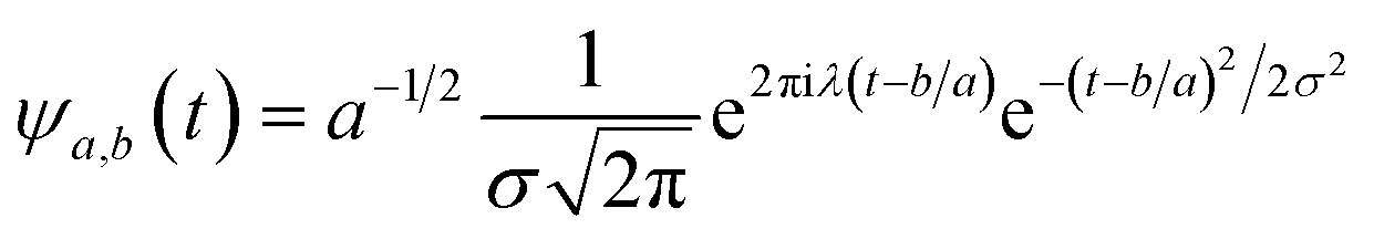
 , and λ = 1 and σ = 2 are the values for constants. These parameters are adjusted to get better resolution in the calculated frequencies. The snapshots of trajectory frames undergo Fourier transformation76 of time-domain data to generate frequencies. Wavelet code runs through the entire trajectory and computes the frequency77,78 of all OD modes.